Joint State and Parameter Estimation by Extended Kalman Filter (EKF) technique

e-ISSN: 2278-067X, p-ISSN: 2278-800X, www.ijerd.com

Volume 11, Issue 08 (August 2015), PP.42-52

Joint State and Parameter Estimation by Extended Kalman

Filter (EKF) technique

1

S. Damodharao,

2

T.S.L.V. Ayyarao

1

PG Student, Dept. of EEE, GMR Institute of Technology Rajam, Andhra Pradesh, India 2

Assistant Professor, Dept. of EEE GMR Institute of Technology Rajam, Andhra Pradesh, India

Abstract:- In order to increase power system stability and reliability during and after disturbances, power grid global and local controllers must be developed. SCADA system provides steady and low sampling density. To remove these limitation PMUs are being rapidly adopted worldwide. Dynamic states of power system can be estimated using EKF. This requires field excitation as input which may not available. As a result, the EKF with unknown inputs proposed for identifying and estimating the states and the unknown inputs of the synchronous machine.

Index Terms:- Dynamic state estimation, extended kalman filter, state estimation, synchronous generator.

I.

INTRODUCTION

Harmonic injection has been a increasing power quality concern over the years. With the growing the use of power electronic devices, the maintenance of power quality has become a major problem for the electric utility companies [6]. But high-performance monitoring and control schemes can hardly be built on the existing SCADA system which provides only steady, low-sampling density and non synchronous information about the network. SCADA measurements are too infrequent and non synchronous to capture information about the dynamic system. It is to remove these limitations that wide area measurements and control systems (WAMAC) using phasor measurement units PMUs) are being rarely adopted worldwide.

The wide area measurement system (WAMS) developed rapidly in most of the years. It has been applied to the monitoring and control of power systems. But as a kind of measurement system, WAMS has the measurement error and not convinent data unavoidably [3]. The steady measurement errors of WAMS have been prescribed in corresponding IEEE standard, but the dynamic measurement errors now become the focus of discussion. If the dynamic raw data is applied directly, the unpredictable consequence will be resulted in, which will damage to power systems. Therefore, the dynamic state estimation for the state variables during electromechanical transient process is the backbone for dynamic applications and real-time control.

A number of papers have focused on just one dynamic state of the power system at a time, typically the rotor angle or speed which was estimated such as neural networks and AI methods. These AI-based model-free estimators generate the estimated rotor speed or rotor angel signal without requiring a mathematical model or any machine parameters [1-2]. In the large-scale power system stability analysis, it is often preferable to have an exact model for all elements of the power system network including transmission lines, transformers, Induction motors, and also synchronous machines. Therefore, the physical model-based state estimator of the generator including voltage states in addition to rotor angle and speed would be more interesting in system monitoring and control.

Synchronized phasor measurement units (PMUs) were introduced, and since then have be-come a mature technology is used with many applications which are currently under development around the world. The occurrence of major problems in many major power systems around the world has given a new impetus for large-scale implementation of wide-area measurement systems (WAMS) using PMUs and Phasor data concentrators (PDCs) [4]. Data provided by the PMUs are very accurate and enable system analyzing to determine the exact sequence of events which have led to the problems. As experience with WAMS is gained, it is natural that other uses of phasor measurements will be found. In particular, significant literature already exists which deals with application of phasor measurements to system monitoring, protection, and control. The most common technique for determining the phasor representation of an input signal is to use data samples taken from the waveform, and apply the discrete Fourier transform (DFT) to compute the phasor measurement. Since sampled data are used to represent the reference signal, it is essential that ant aliasing filters be applied to the reference signal before data samples are taken. The ant aliasing filters are analog devices which limit the bandwidth of the pass band to less than half the sampling frequency.

Fig.1 compensating for signal delay introduced by the ant aliasing Filter

Synchrophasor is a term used to describe a phasor which hasbeen estimated at an instant. In order to obtain simultaneous measurement of phasors across a wide area measurement of the power system, it is necessary to synchronize these time tags, so that all Phasor measurements belonging to the same time tag are truly. Consider the marker in Fig. 1 is the time tag of the measurement. The PMU must then provide the phasor given by using the sampled data of the input signal. Furthermore, this delay will be a function of the signal frequency [7]. The task of the PMU is to compensate for this delay because the sampled data are taken after the ant aliasing delay is introduced by the kalman filter. The synchronization is achieved by using a sampling clock pulse which is phase-locked to the one-pulse-per-second signal provided by a GPS receiver. The receiver may be built in the PMU, or may be installed in the substation and the synchronizing pulse distributed to the PMU and to any other device. The time tags are at intervals that are multiples of a period of the nominal power system frequency.

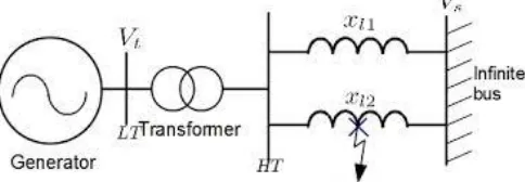
II. SINGLE-MACHINE INFINITE-BUS POWER SYSTEM

A general power system can be simplified to an equivalent circuit system with a single machine connected to an infinite bus via transmission lines. The so-called single machine infinite-bus (SMIB) system, shown in Fig. 2, will be the basis for developing and validating our generator state estimates. Assuming a classical synchronous generator model, let define as the rotor angle by which, the q-axis component of the

Fig. 2. Synchronous machine connected to an infinite bus via transmission lines.

Voltage behind transient reactance, leads the terminal bus. If the terminal voltage can be chosen as the reference phasor. The 3 phase generator can generate 3 phase voltages and currents can be connected to the infinite bus through the transformers and transmission lines. The transformers can be stepped up the voltage. The rotor angel and rotor speed can be estimated by the synchronous machine. The generator in Fig. 2 can then be represented in the dqo domain by the following eight-order nonlinear equation:

The state variables and state vectors are calculated as:

(1)

(2) State variables are described by equations are:

(3)

(4)

(5)

T

x

x

x

x

ed

eq

X



[







]



[

₁

₂

₃

₄

]

T

fd

m

E

u

u

T

u



[

]



[

_{1 2}

]

2 0 .

1

w

x

x



)

(

1

2 1

.

2

u

T

Dx

j

x





_e



)

)

(

(

1

1 3

2 0 .

3 d d d

d

i

x

x

x

u

T

(6)

x



₅



0

(7)

x



₆



0

(8)

x



₇



0

(9)

x



₈



0

(10)

Where

w

₀ is the nominal synchronous speed (elec.rad/s), the rotor speed (p.u),

T

_m the mechanical input torque (p.u),

T

_e the air-gap torque or electrical output power (p.u),

E

_fdthe exciter output voltage or the field voltage as seen from the armature (pu), and



the rotor angle in (elec.rad). Other variables and constants are defined. Based on the phasor diagram associated to the network the air-gap torque will be equal to the terminal electrical power (or) neglecting the stator resistance is zero:

T

_e



P

_t



R

_a

i

2



e

_d

i

_d



e

_q

i

_q (11)

where the d-and q-axis voltages can be expressed as

e

e

d q t t t q t d V E V e V e 2 2 cos sin        (12)

Also, the d-axis and q-axis currents are

i

i

d q t q t q d t d

I

x

x

V

i

x

x

V

x

i

2 2 1 1 1 3

sin

cos











(13)

Using (3) and (4) in (2) and after some mathematical simplifi-cation, the electrical output power at terminal bus with the state variables and can be obtained as: ₁ 1 2 1 3 1

2

sin

)

1

1

(

2

sin

x

x

x

V

x

x

x

V

P

T

d q t d t t e









(14)

The output powers (

P

_t

,

Q

_t) are ₁ 1 2 1 3 1

2

sin

1

1

2

sin

x

x

x

V

x

x

x

V

P

d q t d t t























(15)

_





















q d t d t t

x

x

x

x

V

x

x

x

V

Q

1 2 1 1 2 2 1 3 1

sin

cos

2

cos

(16)

Assumptions are: 37 . 0 , 37 . 0 , 21 . 1 , 06 . 2 01 . 0 , 13 . 0 , 10 , 05 . 0 29 . 2 , 8 . 0 , 02 . 1 1 1 0 0            q d q d q d fd m t x x x x T T J D E T V

)

)

(

(

1

1 4 0 .

4 q q q

q

i

x

x

x

T

The steady state equations at

x

₁.

,

x

₂.

,

x

₃.

,

x

.₄

,

x

₅.

,

x

₆.

,

x

₇.

,

x

₈.



0

To found the values of

x

₁

,

x

₂

,

x

₃

,

x

₄

3998

.

0

0983

.

1

0

6

.

0

4 3 2 1



















d q

e

x

e

x

x

x





(17)

The above assumptions to find the values of

i

_d

,

i

_q

475

.

0

693

.

0





q d

i

i

The air gap torque (or) electrical power can be calculated as:

T

e



P

t



0

.

8

The output powers can be calculated as:

05

.

0

8

.

0





t t

Q

P

III. LINEAR AND NONLINEAR MODELS

Kalman Filter, Extended KF, Unscented KF (UKF) are models popularly used for state estimation process. The traditional Kalman Filter is optimal only when the model is linearized.

STATE SPACE MODELS

A state space model is a mathematical model of a process, where state x of a process is represented by a numerical vector.

A. Non linear State Space Model

The most general form of the state-space model is the Non linear model. This model typically consists of two functions, f and h:

x_{k+1 =} f (x_k,u_k,w_k) (18)

z_k = h(x_k,v_k) (19)

B. State estimation

Fig 4: Mathematical view of state estimation

The most general form of an state estimation is known as Recursive Bayesian Estimation. This is the optimal way of analyzing a state pdf for any process, given a system and a measurement model.

IV. KALMAN BASED FILTERS

A. Kalman and Extended Kalman filter

The problem of state estimation can be made manipulable. If we put certain constrains on the process model, by requiring both ‗f‗ and ‗h„to be linear functions, and the Gaussian and white noise terms ‗w‗ and ‗v„to be uncorrelated, with zero mean. Put in mathematical notation, we then have the following constraints:

f (xk, uk, wk) = Fkxk +Bkuk +wk (20) h (xk, vk) = H xk +vk (21) The constraints described above reduce the state model to:

xk+1 = Fkxk +Bkuk +wk (22) zk = Hk xk +vk (23)

Where F, B and H are time dependent matrices.

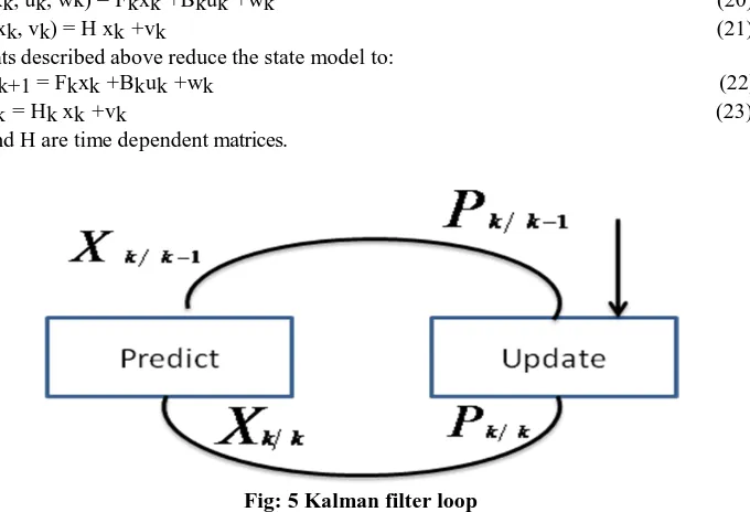
Fig: 5 Kalman filter loop

The recursive Bayesian estimation technique is then reduced to the Kalman filter, where f and h is replaced by the matrices F, B and H. The Kalman filter is, just as the Bayesian estimator, decomposed into two steps: predict and update. The actual calculations required are:

Predict next state, before measurements are taken:

k|k−1 = Fk k−1|k−1+Bkuk (24)

Pk|k−1 = FkPk−1|k−1F T +Qk (25)

B. EKF Algorithm Description

To derive the discrete-time EKF algorithm, we start from the basic definition of time derivation of a variable x:

(26)

where t is the time step, and indicate the time at 0,1….and , or respectively.

(27)

(28)

Where

x

_Kis the system state vector, is the known input vector of the system, is either the process (random state) noise or represents inaccuracies in the system model, is the noisy observation or measured variable (output) vector, and is the measurement noise.

Steps to improving the state estimation:

1. Initialize state vector and state covariance matrix

X= [0; 0; 0; 0; 0.19; 0.04; 8; 0.01];

P=diag ([1^2, 0, 10^2,1^2,0.19,19.297^2,0,10^2]); (29)

Q=diag ([0.08^2, 0.08^2, 0.08^2,0.09^2,0.08^2,0.08^2,0.19^2,0.09^2]);

R= ([0.1^2 0 0 ; 0 0.1^2 0; 0 0 0.1^2]);

2. Compute the partial derivative matrices:

(30)

3. Predict state vector and state covariance

(31)

4. Update error covariance

(32) 5.Perform the gain matrices and update the state vector

(33) DISCUSSION:

x

x

x

f

F

k k

k













 1 1

=









,

,





_1







k

x

w

u

x

f

t

x

(34)

               

T

x

k

x

x

k

x

x

k

x

x

k

x

x

k

x

x

k

x

x

k

x

x

k

x

F

_k

_



_





































1 1 2 3 4 5 6 7 8

(35)

 

₁



,

,



₁



1



1

k





t



f

x

u

w



x

k



x

t k x k x x   

 ( ) ( 1)

.

)

,

,

(

.

)

1

(

)

(

k

x

k

t

f

x

u

w

x









1

)

,

,

(

.



_





K

K

t

f

x

u

w

X

x

0 0,p

X        1 1 1 k k k x x f

F  

 

k k

k x _x

h

H

) ( _1 



_f

_x

x

k _k k

Q F P F P T k k k

k  

    1 1  _{ }

P

H

K

P

k [1 k k] k

1

]

[  







_P

_H

_H

_P

_K

K

k k k

T

k k k

 





,

0



 

_

_

_

k k k k k

k

x

K

y

h

x

 

 

 

 

 

 

 

 

 

                         8 1 7 1 6 1 5 1 4 1 3 1 2 1 1 1 1 x k x x k x x k x x k x x k x x k x x k x x k x x k

x 1 

_

_{11 12 0 0 0 0 0 0}

_

F F x x _k    (34)

x

₂

 

k





t



f

₂



x

,

u

,

w





x

₂



k



1



 

₃



,

,



₃



1



3

k





t



f

x

u

w



x

k



x

 

_

_

0 27 26 0 0 23 22 21 2 F F F F F x

x k _

  (36)  

_

_

0

0

0

35

0

33

0

31

3

F

F

F

x

x

k

_





 

₄



,

,



₄



1



4

k





t



f

x

u

w



x

k



x

 

_

_

48 0 0 0 44 0 0 41 4 F F F x x k _



 ₍₃₇₎

x

5

 

k





t



f

5



x

,

u

,

w





x

5



k



1



 

_

_

0 0 0 55 0 0 0 51 5 F F x x k _



 ₍₃₈₎

x

6

 

k





t



f

6



x

,

u

,

w





x

6



k



1



 

_

_

0 0 66 0 0 0 0 61 6 F F x

x k _

 

(39)

x

7

 

k





t



f

7



x

,

u

,

w





x

7



k



1



 

_

_

0 77 0 0 0 0 0 71 7 F F x x k _



 ₍₄₀₎

x

₈

 

k





t



f

₈



x

,

u

,

w





x

₈



k



1



 

_

_

88 0 0 0 0 0 0 81 8 F F x

x k _

 

(41)

F11=1

0

12

dt

w

F







 

 

 

cos



2

 

1



1 1 1 1 cos 1 3 7

21 2 _X

xd x V X xd X V X dt F q t t                    

  1

7 6 22  

X X dt F

 

sin

 

1 1 7 23 X xd V X dt

F  t

   

2 7

26 X

X dt F 

 

_



 

 

 



_ __  _



 

    

  _ 

 sin2 1 6 2

1 1 1 2 1 1 sin 3 7 27 2

2 X X X

xd xq V xd X X V T X dt

F m t t

  



1

 

1 sin 5 31 1 xd X V x x X dt F t d d   

 





     _    1 1 5 1 33 1 xd x x X dt

F d d

 

  

  

 

            1 1 2 1 cos 3 3 5 35 d t d d fd x X V X x x X E X dt

F





 

q t q q q x X V x x T dt

F41 1 cos 1

0   1 44 0    q T dt F

 

 





 

_           q t q q x X V x x X X dt

F 4 sin 1

8

48 _{2 1}

F55=1 F66=1 F77=1 F88=1

For calculating the

H

_k matrix, we same as the

F

_k1,the output equation of the system is



k k k



k

k

h

x

u

v

And for calculating

H

_k T k

x

h

x

h

x

h

H























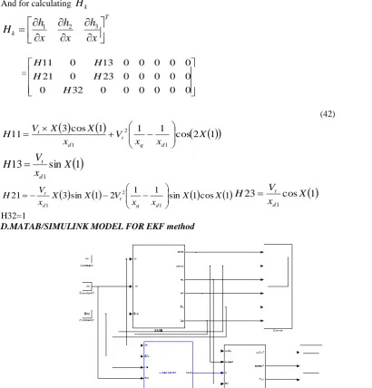
1 2 3

=           0 0 0 0 0 0 32 0 0 0 0 0 0 23 0 21 0 0 0 0 0 13 0 11 H H H H H (42)

 

 

_

_{ }

_

1 2 cos 1 1 1 cos 3 11 1 2 1 X x x V x X X V H d q t d t            

 

1

sin

13

1

X

x

V

H

d t



 

3 sin

 

1 2 1 1 sin

 

1 cos

 

1 21 1 2 1 X X x x V X X x V H d q t d t           



23

cos

 

1

1

X

x

V

H

d t



H32=1

D.MATAB/SIMULINK MODEL FOR EKF method

Fig 6: MATLAB/SIMULINK for EKF

E. EKF Method Simulation Results

The EKF algorithm was developed in Simulink using then embedded function block, just as we did for the EKF method. In the latter case, was the only measurable output signal and were the three input signals. But in the EKF method, and are the three output measurements and the input signals and are still necessary. The input is now assumed to be accessible or known. The initial values vector for states is and for the gain factor matrix is . The initial values related to the unknown input are: and

. Also, the mean and covariance of the state and output noise matrices are as: To better reflect real system conditions, white noise was added to the state with (mean, covariance) and to the measured output with (mean, covariance) under these assumptions, the results of the EKF algorithm for online state estimation of the fourth order nonlinear model of the synchronous generator subjected to a step on are presented in Fig. 4(a). The estimated output signals and the unknown input estimate are also shown in Fig. 4(b) and (c), respectively.

. ] 0 , 0 , 0 , 0 , 0 , 0 , 0 , 0 [ 0  X ] 2 ^ 10 , 2 ^ 10 , 2 ^ 10 , 2 ^ 10 , 10 , 10 , 10 , 10

[ 2 2 2 2

0 

A. Rotor angel in rad estimation

In EKF, the actual value of delta is 0.6.observering from the estimated value is 0.59.The dynamic state of power system at the steady state value after applying the non-linear state estimator to get the steady state value is 0.598. It‟s to be get the system be stabilized. The figure is drawn between the rotor angle actual to the estimated value.

B. Rotor Speed rad/sec estimation

In EKF, the actual value of change in speed is 1.102.observering from the estimated value is 1.108.The dynamic state of power system at the steady state value after applying the non-linear state estimator to get the steady state value is 1.108. It‟s to be get the system be stabilized. The figure is drawn between the rotor speed actual to the estimated value.

In EKF, the actual value of Eq in p.u is 1.102. observe ring from the estimated value is 1.107.The dynamic state of power system at the steady state value after applying the non-linear state estimator to get the steady state value is 1.107. It‟s to be get the system be stabilized. The figure is drawn between the Eq actual to the estimated value

D.

E

D IN P

.

U ESTIMATION

FIG

7:

EKF STATE ESTIMATION WITH RESULTS

(

A

)

ROTOR ANGEL

,

(

B

)

ROTOR SPEED

,

(

C

)

EQ ESTIMATION

,(

D

)

ED ESTIMATION

In EKF, the actual value of Ed in p.u is 0.4. observe ring from the estimated value is 0.399.The dynamic state of power system at the steady state value after applying the non-linear state estimator to get the steady state value is 0.399. It‟s to be get the system be stabilized. The figure is drawn between the Ed actual to the estimated value.

F.JOINT STATE AND PARAMETER ESTIMATION:

(8.a) D in p.u estimation

(8.b)Tdo in p.u estimation

Fig 8: Joint state and parameter estimation results(a),(b)

In EKF, the actual value of Tdo in p.u is 0.13. observe ring from the estimated value is 0.44.The dynamic state of power system at the steady state value after applying the non-linear state estimator to get the steady state value is 0.43. It‟s to be get the system be stabilized. The figure is drawn between the D actual to the estimated value. The states are observed by the scope to be jointed to the extended kalman filter. The subsystem which consists of the SMIB to the kalman filter. The errors of D, J, Tq0, and Tdo can be observ

V. CONCLUSION

In this paper, dynamic state estimation of a power system including the synchronous generator rotor angle and rotor speed. The approach was the traditional nonlinear state estimator, the EKF method, which includes linearization steps in its algorithm. Simulation results of the EKF estimator showed appropriate accuracy in estimating the dynamic states of a saturated fourth-order generator connected to an infinite bus, under noisy processes. The developed EKF-based estimators were effective as well under network fault conditions with process and measurement noise included. The joint state and parameter estimation results were some noised.

REFERENCES

[1]. Esmaeil Ghahremani and Innocent Kamwa “Dynamic State Estimation in Power System by Applying the Extended Kalman Filter With Unknown Inputs to Phasor Measurements”, IEEE Transaction on PS, VOL.26,Feb 2011.

[2]. P. Kundur ”Power System Stability and Control”,

[3]. Xiaohui Qin, Baiqing Li and Nan Liu Power System Department, China Electric Power Research Institute, “Dynamic State Estimator Based on Wide Area Measurement System During Power System Electromechanical Transient Process,” IEEE Neural Network Conf. (IJCNN) 2004.

[4]. Jaime De La Ree, Virgilio Centeno, James S. Thorp, and A. G. Phadke, “Synchronized Phasor Measurement Applications in Power Systems,” IEEE Trans. Power App. Syst., vol.24, pp. 1670–1678, 2010.

[5]. PengYang,ZhaoTan, IEEE, Ami Wiesel, Member, “Power System State Estimation Using PMUs With Imperfect Synchronization,” 2010

[6]. Kent K. C. Yu, N. R. Watson, and J. Arrillaga, “An Adaptive Kalman Filter for Dynamic Harmonic State Estimation and Harmonic Injection Tracking,” Proc. 2009 Power & Energy Society Meeting (PES2009),MAY 1995.

[7]. G. Valerie and V. Terzija, “Unscented Kalman filter for power system dynamic state estimation,” IET Gen., Transm. Distrib., vol. 5, no. 1, pp. 29–37, 2011.

[8]. J. Chang, G. N. Taranto, and J. Chow, “Dynamic state estimation in power system using gain-scheduled nonlinear observer,” in Proc. 1995 IEEE Control Application Conf, pp. 221–226.

[9]. S. Gillian‟s and B. De Moor, “Unbiased minimum-variance input and state estimation for linear discrete-time systems,” Automatica, vol. 33, no. 4, pp. 111–116, 2007.