1. Design and analysis of wavelet based sharpening filter for interpolated images

(1)

DESIGN AND ANALYSIS OF WAVELET BASED SHARPENING

FILTER FOR INTERPOLATED IMAGES

F. Taher1, A. Al-Maazmi2, Alavi Kunhu3, H. Al-Ahmad4

1. INTRODUCTION

Improving the image pictorial information for human and machine interpretation in satellite images has been always a great aim in digital image processing with high resolution. Resolution basically means the ability of an imaging system to record fine detail in a distinguishable manner. In satellite images, these imperfections can be represented as non-symmetric factors such as scene characteristics noise, atmospheric condition such as clouds, illumination and system deterioration [1]. Therefore, an image with greater details and information has higher resolution. The four types of resolution are: spatial, spectral, temporal and radiometric. Spatial resolution of a digital image is defined as the pixel intensity in an image which can be measured by both the number of pixels per unit area or the number of sensor elements per unit area. Low-resolution (LR) images that are resulted from insufficient imaging sensors density, suffer from low spatial sampling frequency aliasing. High resolution (HR) images can be easily obtained from a large number of imaging sensors, however these sensors can be costly and not compatible with the satellite pay load. Moreover, once the satellite is launched it is impossible to change these satellite imagery sensors. Hence, image resolution is limited due to previous mentioned issues [2]. Therefore, signal processing algorithms that provide means to obtain high-resolution images are needed. These algorithms are known as super-resolution (SR) reconstruction algorithms. The driving idea behind SR algorithms is to obtain high-super-resolution images from some low-resolution images by joining the non-excess information in LR images.

One of the fundamental approaches of SR reconstruction is interpolation. Interpolation is the process of increasing the image size. However, in this process, some of the frequencies components cannot be recovered due to the insufficient number of available information. The basic principle of SR reconstruction algorithm depends on the reveres process of getting LR. Several LR images are captured; these LR images are down-sampled from the high resolution image with sub-pixel shifts. After that, the SR reconstruction algorithm reverses the previous unwanted effect by aligning the low resolution observations to sub-pixel accuracy. At the end, the results are combined into a bigger image grid to generate a high resolution image. Super-resolution techniques can be designed in both spatial and frequency domain algorithms. The spatial domain algorithms are more common due to its simplicity compared with the frequency domain algorithms. The latter is used due to robustness and computation efficiency. The algorithm which is used in this work uses the wavelet transform for getting SR images from LR images [2].

The aim of this paper is to document the effort on improving SR algorithm that was developed in [3] to obtain an HR image from a single LR image. The modification on the algorithm is implemented on satellite images. The problem is approached using the interpolation and filtering principles to enhance either the whole image or specified segments of the image. Optimization techniques are used in the design of the resulted filters. The performance of the modified algorithm versions is evaluated by scaling down an HR image which represents the ground truth. Then, interpolation and filtering is implemented

1_{College of Technological Innovation, Zayed University, Dubai, U.A.E}

2_{Khalifa University, Abu Dhabi, U.A.E}

3_{College of Engineering and IT, University of Dubai, UAE} 4_{College of Engineering and IT, University of Dubai, UAE}

DOI: http://dx.doi.org/10.21172/1.131.11

e-ISSN:2278-621X

Abstract: Satellite images have been used in many applications and fields of research. One of the major limitation of satellite image is their resolution. This paper proposes a new satellite image resolution enhancement algorithm, based on the design and analysis design of new sharpening filters, by obtaining their discrete wavelet transform to improve interpolated images. The sharpening filters are intended for a particular image by means of reducing the image resolution, and then enlarging it. The enlarged interpolated image and the ground truth image are decomposed into four wavelet components LL, LH, HL, and HH. These four components are compared peer to peer and used to design and obtain the sub-optimum sharpening filter kernels that maximize the peak signal to noise ratio, and ultimately, create a super resolution image. Proposed algorithm is based on cross shaped sharpening filters and the performance of the algorithm evaluated using the peak signal to noise ratio (PSNR). The evaluation process compared the wavelet sharpened interpolated images to the ground truth images. The resulted output images showed in a significant improvement compared with interpolation methodology only, without losing any information content present in the satellite image.

(2)

The main problem in LR images that they suffer from the reverse effects of blurring, under-sampling, and wrapping. Super resolution algorithms objectives are to overcome these problems. The single image interpolation methods have limited capabilities to recover image details that appear in high frequency components. The authors in [5] have developed an interpolation algorithm that overcomes the varying illumination influence during the interpolation process and reducing the effect of jaggy-noise in the interpolated image edges. This super resolution algorithm is based on edge adaptive enhancement. The algorithm developed in [6] is based on allowing the restoration process to take a full advantage of all prior knowledge by maximizing a posterior probability estimator, maximum likelihood, and using the concept of projection onto convex sets. It is worth mentioning that this algorithm uses frequency domain techniques in its process. The authors in [7] proposed an algorithm to enhance the interpolated image. However, their algorithm suffers from several limitations such as the fact that the improvement provided by the algorithm is dependent on the image category and the quality measure chosen. Also, the algorithm is sensitive to the noise.

Another algorithm developed in [8] uses an iterative approach in order to increase the color images resolution. The algorithm performs well with both natural images and computer simulated images. The algorithm relies on a set of LR images (also known as a dictionary) which were produced by simulating the input image. After that the difference images are used to improve the initial prediction using “Back-Projecting” method. Thus, the error is minimized by iterating this process. The algorithm proposed in [9] increases the image resolution by using two linear arrays of sensors on-board satellite and increasing the sampling frequency. The algorithm developed in [10] is based on obtaining multiple under-sampled images of a scene. Then the image sensors that were used to acquire the image are shifted by sub-pixel displacement relative to each other. However, the algorithm is not capable of incorporating the spectral correlation of the three basic colors which is considered a major limitation of the algorithm. However, the algorithm proposed in [10] obtains SR images by using adaptive Wiener filter. The algorithm results minimum error, in addition to its computational simplicity compared with other algorithms. The authors in [11] developed an algorithm that works by combining LR images to get a HR image. The algorithm main advantage is its ability to remove geometric distortion on image shape. It is worth to note the algorithm is suitable for real time application because it uses a non-uniform interpolation which reduces the computational complexity.

3. INTERPOLATION TECHNIQUES AND ASSESSMENT

Interpolation is the process of estimating the pixel values for unknown locations using known pixels. Its main concept resembles the image. The resembling is the process which the pixel values are reassigned and sampled according to the new position. Sampling methods includes nearest neighborhood, bilinear interpolation and cubic convolution. In nearest neighborhood, it simply selects the digital value of the nearest pixel to the selected point at the original image. The bilinear interpolation calculates the average of four nearest pixels to the selected point at the original image. Finally, the cubic convolution uses 16 pixels to calculate the new pixel. The nearest neighborhood is the simplest approach among them as each pixel by pixel is rotated rather than taking a group of pixels which cases resolution decrement [12].

Image processing techniques might result in losing some information from the processed image. A lossy image is an image that loses some of the information and pixels details in the processing. Although human eyes can judge on the performance of the processing subjectively by inspecting the resultant images; however, in order to obtain the quality of the image objectively, PSNR is used. PSNR is the peak signal to noise ratio that can be used for comparison purposes for image quantity evaluation. The PSNR between two images A and B is defined using the following equations [4]:

( , ) = 10 log10 ( ( , )2552) ( , ) = 1 ∑ =1 ∑ =1( − )2

Where MSE(A,B) is the mean square error between image A, and B. It is worth to note that PSNR increases as MSE decreases. It is desirable to have high PSNR ratios, the higher the numerical number, the better indication.

4. SUB-OPTIMUM SHARPENING FILTERS FOR GREY-SCALE IMAGES

Initially, the size of the image will be reduced by a factor of 2 using different interpolation methods. Then both interpolated and the ground truth image will be divided into four frequency components of wavelet, which are LL, LH, HL and HH. Each of these components of the interpolated image will be compared to its peer from the original image to create a sub-optimum cross shaped spatial filter that maximizes the PSNR by minimizing the MSE. The Figure 1 shows the linear phase two-dimensional sharpening filter which include a sliding window. The main advantage of this sharpening filter is the simplicity of design where two coefficients are needed to know a1 and a2, while a3 is calculated using the below equation:

(3)

Figure 1. 5x5 Sharpening Filter

A different filter will be implemented for each part, hence resulting four filters. These filters are used to filter the wavelet components of the interpolated image. Finally after filtering, the wavelet components are recomposed again by using the inverse of discrete wavelet transform to construct high resolution image. The process can be implemented for higher order filters such as 7x7, 9x9 or 11x11. Each part in the image has its own distinguished sharpening filter. The algorithm is tested on different gray-scale satellite images. In all cases, the size of the tested images is 512x512 pixels. In the first case, initially, the size of the original 1024x1024 image is decreased to 512x512. Figure 2 shows the block diagram of the proposed method in [3]. That can be used as a base to develop an algorithm with discrete wavelet transform.

Figure 2. Block Diagram of the Proposed Method

5. RESULTS AND DISCUSSION

The quality assessment method that is used to assess the enchantment in the resultant images is peak signal to noise ratio (PSNR). The PSNR is calculated between the original image and the high-resolution image. The comparison cannot be directly implemented as the original and resulted image have of different resolutions, and the corrected magnified image is unknown. Therefore, the original image can be downsized to generate a lower resolution version and then upsized to magnify it. The original image called the ground truth [15]. In reality, this image is not provided, however in this paper it is used for comparison purposes. The algorithm was testing and implemented on various gray scale satellite images. Each image will result in different PSNR according to its own designed filter that minimize the MSE. There are three cases of comparison which are: original with interpolated image, original with applying sub-optimum filter designed in the spatial domain and original with applying sub-optimum filter designed in the wavelet domain. The comparison also included different interpolation techniques such as nearest, bi-linear, bi-cubic, Lanczos2 and Lanczos3.

(4)

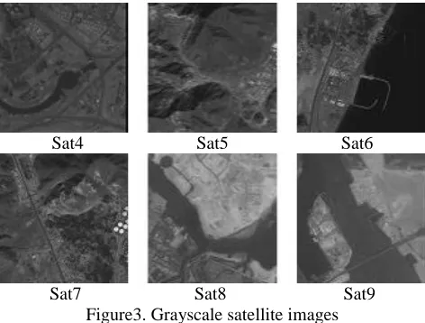
Sat4 Sat5 Sat6

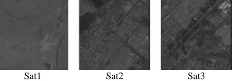
Sat7 Sat8 Sat9 Figure3. Grayscale satellite images

Nearest neighbor: First results are the output images when nearest neighbor interpolation is used. In the nearest neighbor algorithm, the pixel value is approximated by the value of the nearest pixel, discarding the neighboring points. Table 1 and 2 shows the results of the algorithm by using nearest neighbor interpolation.

Table 1. PSNR analysis of algorithm using nearest neighbor interpolation

Image

PSNR (in dB)

Interpolation Only Sub-optimum filter in spatial Sub-optimum filter in wavelet

Sat1 41.6443 43.3639 42.3297

Sat2 33.7193 35.5662 34.4256

Sat3 34.244 36.1301 34.9444

Sat4 35.6063 37.3869 36.327

Sat5 34.4045 36.4759 35.0742

Sat6 34.848 36.8602 35.4202

Sat7 33.5154 35.6109 34.1235

Sat8 36.6891 38.8823 37.2594

Sat9 38.7053 40.8147 39.2843

From Table 1 and 2, we can conclude that that proposed method does show a slight improvement over the interpolation only, however, using the suboptimum filter in the spatial domain, has better PSNR and SSIM over both interpolations only and suboptimum filter in wavelet domain using 2D-DWT. This attribute can be seen clearly from all satellite images. Figure 4 and 5 shows the resultant satellite images when applying the algorithm by nearest neighbor interpolation.

Table 2. SSIM analysis of algorithm using nearest neighbor interpolation

Image

SSIM

Sat1 0.9941 0.9938 0.9916

Sat2 0.9800 0.9793 0.9729

Sat3 0.9838 0.9834 0.9783

Sat4 0.9873 0.9869 0.9829

Sat5 0.9872 0.9872 0.9828

Sat6 0.9893 0.9893 0.9849

Sat7 0.9848 0.9850 0.9789

Sat8 0.9906 0.9909 0.9876

(5)

Zoomed Interpolated Sat2 Zoomed Interpolated Sat4

Zoomed Spatial filtered Sat2 Zoomed Spatial filtered Sat4

Zoomed Wavelet filtered Sat2 Zoomed Wavelet filtered Sat4 Figure 4. Sat images with nearest neighbour interpolation

Interpolated Sat1 Spatial filtered Sat1 Wavelet filtered Sat1

(6)

Interpolated Sat6 Spatial filtered Sat6 Wavelet filtered Sat6 Figure 5. Sat images with nearest neighbour interpolation algorithm

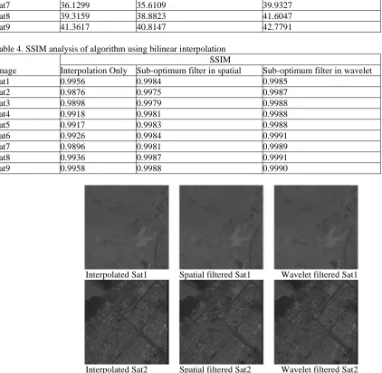
Bilinear: Second results are the output when bilinear interpolation is used. In the bilinear algorithm, the pixel value is approximated by the value weighted average of the four nearest cell centres. Table 3 and 4 shows the results if the algorithm by using bilinear interpolation.

Original image Interpolated image

(7)

From Table 3 and 4, we can conclude that that proposed method does show a slight improvement over the interpolation only, however, using the suboptimum filter without taking wavelet, has better PSNR and SSIM over both interpolation and suboptimum with 2D-DWT. The algorithm with bilinear interpolation shows almost same behaviour of the nearest neighbour interpolation. Figure 6 show the Sat8 satellite image results when applying the algorithm by bilinear interpolation. Similary Figure 7 and 9 shows the resultant satellite images when applying the algorithm by bilinear interpolation.

Table 3. PSNR analysis of the algorithm using bilinear interpolation

Image

PSNR (in dB)

Sat1 43.6666 43.3639 42.9115

Sat2 36.5183 35.5662 39.4123

Sat3 37.1962 36.1301 39.5668

Sat4 38.5689 37.3869 40.1771

Sat5 37.0986 36.4759 40.4343

Sat6 37.4726 36.8602 41.3187

Sat7 36.1299 35.6109 39.9327

Sat8 39.3159 38.8823 41.6047

Sat9 41.3617 40.8147 42.7791

Table 4. SSIM analysis of algorithm using bilinear interpolation

Image

SSIM

Sat1 0.9956 0.9984 0.9985

Sat2 0.9876 0.9975 0.9987

Sat3 0.9898 0.9979 0.9988

Sat4 0.9918 0.9981 0.9988

Sat5 0.9917 0.9983 0.9988

Sat6 0.9926 0.9984 0.9991

Sat7 0.9896 0.9981 0.9989

Sat8 0.9936 0.9987 0.9991

Sat9 0.9958 0.9988 0.9990

(8)

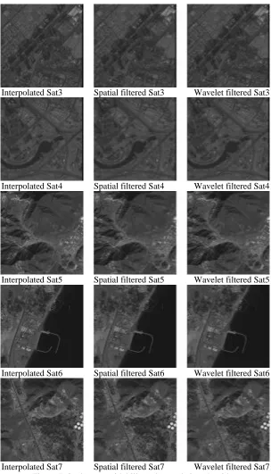
Interpolated Sat7 Spatial filtered Sat7 Wavelet filtered Sat7 Figure 7. Sat images with bilinear interpolation algorithm

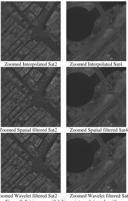
However, some other images such as Sat6 images, show improvement when using sub-optimum filter with 2D-DWT. The Figure 8 images shows the improvements over zoomed parts of Sat6 image.

(9)

Zoomed Wavelet filtered Sat2 Zoomed Wavelet filtered Sat4 Figure 9. Sat images with bilinear interpolation algorithm

Cubic: Third results are the output when the bi-cubic interpolation is used. In the bi-cubic algorithm, the pixel value is approximated by the value of 16 nearest cell centres. Table 5 and 6 shows the results if the algorithm by using cubic interpolation.

Table 5. PSNR analysis of algorithm using cubic interpolation

Image

PSNR (in dB)

Sat1 46.3504 46.6612 46.3329

Sat2 39.746 40.9116 41.7755

Sat3 40.2366 41.2477 41.8701

Sat4 40.2366 41.2477 41.8701

Sat5 40.8461 42.0213 43.0631

Sat6 41.1374 42.4006 43.415

Sat7 39.8287 41.1296 42.146

Sat8 42.9665 43.9373 44.4834

Sat9 44.9445 45.8529 46.0592

(10)

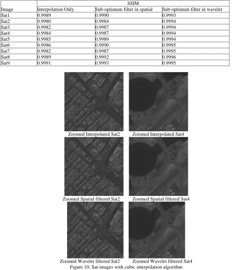
Image Interpolation Only Sub-optimum filter in spatial Sub-optimum filter in wavelet

Sat1 0.9989 0.9990 0.9993

Sat2 0.9980 0.9984 0.9994

Sat3 0.9982 0.9987 0.9994

Sat4 0.9984 0.9987 0.9994

Sat5 0.9985 0.9989 0.9994

Sat6 0.9986 0.9990 0.9995

Sat7 0.9982 0.9987 0.9995

Sat8 0.9989 0.9992 0.9996

Sat9 0.9991 0.9993 0.9995

Zoomed Wavelet filtered Sat2 Zoomed Wavelet filtered Sat4 Figure 10. Sat images with cubic interpolation algorithm

(11)

Original image Interpolated image

Wavelet filtered image Spatial filtered image Figure 11. Sat8 images with cubic interpolation algorithm

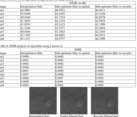
Lanczos-2: The fourth case results are the output when Lanczos-2 interpolation is used. In the Lanczos-2 algorithm, the pixel value is approximated such as pixels are passed into an algorithm that averages their color using sinc functions. Table 7 and 8 shows the results of the algorithm by using Lanczos-2 interpolation.

Table 7. PSNR of the algorithm using Lanczos-2 interpolation

Image

PSNR (in dB)

Sat1 46.4805 46.5922 46.4611

Sat2 39.9468 41.0103 41.9148

Sat3 40.4366 41.3724 42.0378

Sat4 41.3839 42.1476 42.5835

Sat5 41.0395 42.1423 43.1589

Sat6 41.3248 42.5277 43.4694

Sat7 40.0166 41.1843 42.2103

Sat8 43.1383 44.0602 44.5921

Sat9 45.1151 45.9757 46.1589

Table 8. SSIM analysis of algorithm using Lanczos-2

Image

SSIM

Sat1 0.9990 0.9990 0.9993

Sat2 0.9982 0.9984 0.9994

Sat3 0.9984 0.9986 0.9994

Sat4 0.9986 0.9987 0.9994

Sat5 0.9987 0.9989 0.9995

Sat6 0.9987 0.9990 0.9995

Sat7 0.9984 0.9987 0.9995

Sat8 0.9990 0.9991 0.9996

Sat9 0.9992 0.9992 0.9995

(12)

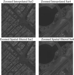
Interpolated Sat7 Spatial filtered Sat7 Wavelet filtered Sat7 Figure 12. Sat images with Lanczos-2 interpolation algorithm

(13)

the filtering process more accurate. Figure 12 and 13 shows the resultant satellite images when applying the algorithm by Lanczos-2 interpolation.

Zoomed Wavelet filtered Sat2 Zoomed Wavelet filtered Sat4 Figure 13. Sat images with Lanczos-2 interpolation algorithm

Lanczos-3: Finally, is to investigate output results when Lanczos-3 interpolation is used. Lanczos-3 is basically Lanczos-2 algorithm but results sharper effect, the pixel value is approximated such as pixels are passed into an algorithm that averages their color using sinc functions. Table 9 and 10 shows the results of the algorithm by using Lanczos-3 interpolation.

(14)

Zoomed Wavelet filtered Sat2 Zoomed Wavelet filtered Sat4 Figure 14. Sat images with Lanczos-3 interpolation algorithm

Table 9. PSNR analysis of algorithm using Lanczos-3 interpolation

Image

PSNR (in dB)

Sat1 47.6168 44.8926 47.6187

Sat2 41.7093 40.9644 42.4612

Sat3 41.9831 41.0749 42.5858

Sat4 42.6421 41.6896 43.1225

Sat5 43.1194 42.2186 43.9868

Sat6 43.2176 42.4541 44.0638

Sat7 41.9925 41.9925 42.9092

Sat8 44.8929 43.6455 45.4711

Sat9 46.8065 45.8877 47.1722

Table 10. SSIM analysis of algorithm using Lanczos-3

Image

SSIM

Sat1 0.9994 0.9993 0.9994

Sat2 0.9994 0.9994 0.9993

Sat3 0.9995 0.9994 0.9993

Sat4 0.9994 0.9993 0.9994

Sat5 0.9995 0.9994 0.9994

Sat6 0.9995 0.9994 0.9994

Sat7 0.9995 0.9994 0.9994

Sat8 0.9996 0.9995 0.9995

(15)

(16)

Interpolated Sat7 Spatial filtered Sat7 Wavelet filtered Sat7 Figure 15. Sat images with Lanczos-3 interpolation algorithm

6. CONCLUSION

A full study was done to understand the super-resolution algorithms and the sub-optimum wavelet filter that maximize the PSNR by minimizing the MSE of each components of the wavelet including LL, LH, HL and HH. The sub-optimum filter was implemented and tested for several interpolation cases with grayscale satellite images. First, it was used to investigate the effect of applying a different filter for each part of the image with and without overlapping. The sub-optimum wavelet sharpening filter is used on satellite images using different interpolation methods and the results vary depending on the satellite image and interpolation methods. The following points can be concluded from our proposed work: Discrete wavelet transform can be used to obtain a sub-optimum filter biased on the wavelet components that maximize the PSNR by minimizing the MSE; The improvement depends on the structure of the image, thus different image will have it is own sharpening filter; The algorithm could be implemented with a variety of interpolation techniques. The cubic, Lanczos-2 and Lanczos-3 interpolation techniques based algorithms gives better result with highest improvement; Cubic, Lanczos-2 and Lanczos-3 interpolation gives a smoothing effect which makes the noise in the image smoothed out, letting the filter results better outputs

7. REFERENCES

[1] http://www.geo.mtu.edu/rs4hazards/ksdurst/website/lectures/RemoteSensing.pdf. [2] P. Milanfar, “Super-Resolution Imaging”, CRC Press; 1st Edition, 2010.

[3] S. A. Al-Nuaimi, “Design and Analysis of Algorithms for Obtaining Super Resolution Satellite Images,” M.S thesis, Dept. [4] Elect. Eng., Khalifa University, Abu Dhabi. Nov. 2013.

[5] Saeed AL-Mansoori and Alavi Kunhu, “Enhancing DubaiSat-1 Satellite Imagery Using a Single Image Super- [6] Resolution”, SPIE of Optics and Photonics Conference 2013, California, USA, August 2013.

[7] X. Wang and H. Ling, "An Edge-Adaptive Interpolation Algorithm for Super-Resolution Reconstruction," International Conference on Multimedia Information Networking and Security (MINES), Jiangsu, China, Nov. 2010, pp.81-84.

[8] M. Elad and A. Feuer, "Restoration of a single super resolution image from several blurred, noisy, and under sampled measured images," IEEE Transactions on Image Processing, vol.6, no.12, Dec 1997, pp.1646-1658.

[9] Begin and F. Ferrie,"Comparison of Super-Resolution Algorithms Using Image Quality Measures," 3rd Canadian Conference on Computer and Robot Vision (CRV'06), Canada, June 2006.

[10] M. Irani and S. Peleg,” Improving Resolution by Image Registration”, Graphical Models and Image Processing Journal, vol.53, May 1991, pp. 231-239.

[11] P. Goudy, P. Kubik, B. Rouge and C. Latry, “From Image Processing Concepts to Instrument Design in Remote Sensing Satellites”, Signal and Image Processing for Space Applications CNES, Vol II, France, pp. 431-434.

[12] M.K. Ng and N.K. Bose, "Mathematical analysis of super-resolution methodology," IEEE Signal Processing Magazine, vol.20, no.3, May 2003, pp. 62-74.

[13] M.T. Merino and J. Nunez, "Super-Resolution of Remotely Sensed Images with Variable-Pixel Linear Reconstruction," IEEE Transactions on Geoscience and Remote Sensing, vol.45, no.5, May 2007, pp.1446-1457.

[14] R. C. Gonzalez and R. E. Woods, Digital Image Processing 2/E. Upper Saddle River, NJ: Prentice-Hall, 2002, pp. 349-404.

[15] M. Kociolek, A. Materka, M. Strzelecki, and P. Szczypinski, "Discrete wavelet transform – derived features for digital image texture analysis”, International conference on Signals and Electronic systems, Lodz, Poland, Sep. 2001, pp.163-168.

[16] P.Y. Lin, "An introduction to Wavelet transform"

[17] Sonja and Mislav, "The Use of Wavelets in Image Interpolation: Possibilities and Limitations," Radio Engineering, vol. 16, no. 4, Dec. 2007, pp.475-479.