1. INTRODUCTION
Multi view-video-plus-depth format for 3D content representation has been adopted for current and future 3D television technologies e.g. free-viewpoint television (FTV) and Super Multi view (SMV) displays. The gray scale depth image represents the per pixel depth value of the corresponding texture image which is exploited to generate novel views through depth image based rendering (DIBR). In MVD format only few views with their associated depth maps are coded and transmitted. The compression of MVD data is indeed an important activity in 3D television framework and much attention has been devoted to this research area. To efficiently compress MVD data various coding formats have been proposed and new tools have been developed, e.g. Advanced Video Coding (H.264/AVC) has been used in past to encode the texture videos and depth videos independently, also known as simulcast coding. The novel High Efficiency Video Coding (HEVC) is the current state of the art video coding tool. The Joint Collaborative Team on 3D Video Coding Extension Development (JCT-3V) has recently developed extensions of HEVC to efficiently encode multiview videos and MVD data. Multi-view-HEVC (MV-Multi-view-HEVC) extends the Multi-view-HEVC syntax to encode MVD without additional coding tools whereas 3D-Multi-view-HEVC is expressively dedicated to the design of novel coding techniques for MVD. 3D-HEVC encodes the base view with its depth map using unmodified HEVC whereas the dependent views and their depth maps are encoded by exploiting additional coding tools. 3D-HEVC achieves the best compression ratio for MVD data. In this paper we introduced a new model called “Novel Saliency Detection Method” in multi-view videos plus depth assessment.
2. PROPOSED METHOD
The proposed quality metric works in two steps; first, the compression sensitivity map (CSM) of the depth image is computed to locate the pixels which are the most susceptible to compression artifacts. Second, for each compression sensitive pixel (CSP) a histogram of then neighbourhood is constructed and analyzed to determine the quality index. BDQM builds on the key observation that the histogram around a CSP gets flattened when increasing the amount of compression; indeed, compression mostly affects. The sharp discontinuities of the depth image. The proposed algorithm exploits the shape of the histogram to predict depth quality. The proposed method uses the shape of the histogram to predict the quality index. It is known that the boundary regions between objects at different depth levels are susceptible to compression artifacts compared to the homogeneous areas in images. So, the magnitude gradient of the image is use full in evaluating the compression sensing artifacts. The compression sensitivity map is computed from its gradients magnitudes. are the gradients along horizontal and vertical directions and are computed with sobel operators. The gradient magnitude is used to select sensitive depth pixels that are used to estimate the quality index.
2.1 Novel Saliency Detection
1
Associate Professor, Dept. of ECE, GCET, Hyd.,India. Geethanjali College of Engineering & Technology, Hyd., India.
2
Associate Professor, Dept. of ECE, GCET, Hyd.,India. Geethanjali College of Engineering & Technology, Hyd., India. detection model is introduced by utilizing low level features obtained from Stationary Wavelet Transform domain.Firstly, wavelet transform is employed to create the multi-scale feature maps which can represent different features from edge to texture. Then, we propose a computational model for the saliency map from these features. This model is aimed to modulate local contrast at a location with its global saliency computed based on likelihood of the features and also considered local centre-surround differences and global contrast in the final saliency map. Experimental evaluation depicts the promising results from the proposed model by outperforming the relevant state of the art saliency detection models.
Figure: Frame work of Saliency Detection 3. BLOCKDIAGRAM
Figure: Block diagram of depth quality metric BDQM using Saliency Detection Method
The figure block diagram shows complete description of the proposed algorithm blind depth quality metric. BDQM using Saliency Detection Method can be integrated with no-reference image quality metrics to design novel 3D image quality scores that, in addition to texture image also consider the depth image to better estimate the overall quality,
4. IMPLEMENTATION
Step1: The first frame is captured through the camera and after that sequence of frames is captured at regular interval of 33.33msec.
Step2: The RGB colour frames are converted into gray scale images. The conversion from a RGB image to gray is done with:
4.1 Computing compression sensitivity map
It is well known that the boundary regions between objects at different depth levels are highly susceptible to compression artifact compared to the flat homogeneous areas of depth images. Therefore,the magnitude of the depth gradient can be a simple and effective means for evaluating compression sensitivity. Let I be an M _ N depth image. The compression sensitivity map (CSM) of I is computed from its gradient magnitudes as:
Where Gx and Gy are gradients along horizontal and vertical directions and can be computed with Sobel filters. The gradient magnitude can be used to select the compression sensitive depth pixels that will be used to estimate the quality index in the following section.
4.2 Depth quality index
The CSM computed in the previous step is used to estimate the quality of the depth image. The CSPs defined above belong to the sharp discontinuities representing the boundaries between two usually very flat or linearly changing regions at different depth levels. To quantify the effect of compression the neighborhood of the CSPs is examined to determine the smoothness induced by quantization. A local histogram is constructed and analyzed to infer the presence of compression effects. As the CSPs lie on or in the proximity of the boundary between two different depth levels, the histogram appears to be very peaked around two bins. In presence of compression, the depth transitions tend to be smoothed and the effect can be captured by a local histogram where the two peaks are less pronounced and the values are more equally distributed in between. To predict the quality of a depth image we propose to estimate the histogram dispersion by measuring the area which lies on top of the histogram curve the larger the area, the less compressed is depth. An area value is associated to each CSP and then averaged together to compute the final quality index.
The proposed BDQM is tested on a number of standard depth videos undergoing HEVC compression. Each depth video sequence is encoded at6 different compression levels, namely QP=f26,30,34,38,42,46g using version HM 11.0 of the HEV reference software with Main profile. Pearson correlation coefficient (PLCC) for prediction accuracy test and Spearman rank order correlation coefficient (SROCC) and Kendall rank order correlation coefficient (KROCC) for Prediction Monotonicity test. To estimate the prediction error we compute Root Mean Square Error (RMSE) and Mean Absolute Error (MAE) measures. Before computing these performance parameters, according to Video Quality Expert Group (VQEG) recommendations the BDQM predicted scores Q are mapped to PSNR with a monotonic nonlinear regression function. The following logistic function outlined is used for regression mapping:
to assess their quality. Peak Signal to Noise Ratio (PSNR) is usually used to evaluate the quality of depth maps. We compare BDQM with PSNR to evaluate its performance. In the following we employ 5 depth videos from standard sequences in the MPEG and HHI datasets. Peak Signal to Noise Ratio (PSNR) PLCC Pearson Linear Correlation Coefficient, RMSE Root Mean Square Error, MAE Mean Absolute Error.The table shows that the BDQM achieves very high correlation with PSNR in ever experiment with an average PLCC of 0.9920. The SROCC and KROCC are equal to 1 in all experiments as the predicted scores are monotonic.
The average prediction error in terms of RMSE and MAE turns to be 0.29 and 0.25, respectively. All the collected results demonstrate the accuracy of the proposed quality metric To further evaluate the reliability of BDQM the performance parameters have been computed over the entire dataset BDQM can be used not only to rank the quality of different compression levels of the same content but also to compare different scores of different videos. Performance of BDQM over entire dataset.
4.3 Correlation (Pearson, Kendall, Spearman)
Correlation is a bivariate analysis that measures the strength of association between two variables and the direction of the relationship. In terms of the strength of relationship, the value of the correlation coefficient varies between +1 and -1. A value of ± 1 indicates a perfect degree of association between the two variables. As the correlation coefficient value goes towards 0, the relationship between the two variables will be weaker. The direction of the relationship is indicated by the sign of the coefficient; a + sign indicates a positive relationship and a – sign indicates a negative relationship. Usually, in statistics, we measure four types of correlations: Pearson correlation, Kendall rank correlation, Spearman correlation, and the Point-Biserial correlation
Pearson correlation: Pearson r correlation is the most widely used correlation statistic to measure the degree of the relationship between linearly related variables. For example, in the stock market, if we want to measure how two stocks are related to each other, Pearson r correlation is used to measure the degree of relationship between the two. The point-biserial correlation is conducted with the Pearson correlation formula except that one of the variables is dichotomous r correlation relationship
r = Pearson r correlation coefficient
N = number of observations
∑xy = sum of the products of paired scores
∑x = sum of x scores
∑y = sum of y scores
∑x2= sum of squared x scores
∑y2= sum of squared y scores
4.4 Kendall rank correlation:
Kendall rank correlation is a non-parametric test that measures the strength of dependence between two variables. If we consider two samples, a and b, where each sample size is n, we know that the total number of pairings with a b is n(n-1)/2. The following formula is used to calculate the value of Kendall rank correlation
Nc= number of concordant, Nd= Number of discordant
4.5 Spearman rank correlation:
Fig :original image
The gradient magnitude can be used to select the compression sensitive depth pixels that will be used to estimate the quality index.
Fig : Depth image
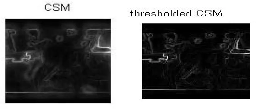
Thresholding by dropping the pixels with CSM is used to locate the most compression sensitive pixels (CSP); please note that this choice has also a positive side effect since it dramatically reduces the computational cost of the whole metric.
Fig : CSM image Fig : Threshold CSM
5.1 Depth Quality Index
Fig :Histogram analysis
The histogram is computed onto 10 equal bins Two very high peaks can observed in it can be noted that the histogram Of the same region exhibits lower peaks and higher valley. The sample histogram of a CSP (neighbourhood of size 15_15) compressed with HEVC .Depth transitions tend to be smoothed and the effect can be captured by a local histogram where the two peaks are less pronounced and the values are more equally distributed in between. showing that the depth values are concentrated around two bins whereas the rest of the histogram is very sparse and almost empty. Histogram / result image:
The shape of the histogram of compression sensitive depth pixels is used to estimate the depth quality in particular, we show that as the compression ratio is increased the histogram around depth transitions flattens because of smoothing. The proposed Algorithm exploits the shape of the histogram to predict depth quality. The higher compression makes the histogram flatter. Depth images are gray scale texture less images usually consisting of large homogeneous or linearly changing regions with sharp edges representing objects’ boundaries. The corresponding depth value to increase the contribution of pixels. The goal of our analysis here is to show that the no reference BDQM can compete with full reference metrics. Since depth maps are texture less gray-scale images the visual image quality metrics are not effective to assess their quality.
3D video image Outputs
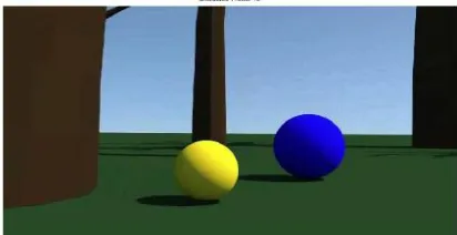
Fig: Original image
Fig: output images 6. DEPTH IMAGE
Depth image in this the original part is going to focused and neglecting the background part. 3D image quality assessment plays important role for the improvement of Compression standards and various 3D multimedia applications. The quality assessment of 3D images. This statement can be verified by the low correlation .To design a System on depth quality assessment and presents a novel algorithm to estimate the distortion in depth videos induced by compression CSM Therefore, the magnitude of the depth gradient can be a simple and effective means for evaluating compression sensitivity.
fig7.8 Historical representation
In depth image histogram of arrivals frequency s are in vertical axis and bin range or time of intervals are per minute (pixels).histogram full presentation In compression sensitivity map (CSM) histogram of arrivals frequency s are in vertical axis and bin range or time of intervals are per minute (pixels).in this the depth of image is going to be less for csm.
Saliency detection model is introduced by utilizing low-level features obtained from the wavelet transform domain. Firstly, wavelet transform is employed to create the multi-scale feature maps which can represent different features from edge to texture. Then, we propose a computational model for the saliency map from these features. The proposed model aims to modulate local contrast at a location with its global saliency computed based on the likelihood of the features, and the proposed model considers local centre-surround differences and global contrast in the final saliency map. Experimental evaluation depicts the promising results from the proposed model by outperforming the relevant state of the art saliency detection models.
7. CONCLUSION
In this paper “Blind Multi-View Videos Plus Depth Assessment Using Novel Saliency Detection Method” has been successfully estimates depth quality by measuring the blurriness of the compression sensitive regions of the depth image using a histogram based approach. The experimental results show that BDQM exhibits high prediction accuracy when compared to full reference PSNR metric. No-reference metric able to rank the compression artifacts of depth maps has been presented. The proposed algorithm leverages on the observation that depth images are characterized by flat regions with sharp boundaries that are potentially blurred after compression.
8. FUTURE SCOPE
BDQM Blind depth quality metric is based on the estimation of the quality of sharp transitions in the depth map it is expected to be a valuable instrument for predicting textural and structural distortions in synthesized images. BDQM is based on the estimation of the quality of sharp transitions in the depth map it is expected to be a valuable instrument for predicting textural and structural distortions in synthesized images.
9. REFERENCES
[1] M. Tanimoto, “FTV: Free-viewpoint Television,” Signal Process.-Image Commun., vol. 27, no. 6, pp. 555 – 570, 2012.
[2] M.P. Tehrani et al., “Proposal to consider a new work item and its use case - rei : An ultra-multiview 3D display, ISO/IEC JTC1/SC29/WG11/m30022, July-Aug 2013.
[3] C. Fehn, “Depth-image-based rendering (DIBR), compression,and transmission for a new approach on 3D-TV,” inSPIE Electron. Imaging, 2004, pp. 93–104.
[4] M. Domanski et al., “High efficiency 3D video coding usingnew tools based on view synthesis,” IEEE Trans. Image Process., vol. 22, no. 9, pp. 3517– 3527, 2013.
[5] M.S. Farid et al., “Panorama view with spatiotemporal occlusioncompensation for 3D video coding,” IEEE Trans.Image Process., vol. 24, no. 1, pp. 205–219, Jan 2015.
[6] T. Maugey, A. Ortega, and P. Frossard, “Graph-based representationfor multiview image geometry,” IEEE Trans. Image Process., vol. 24, no. 5, pp. 1573–1586, May 2015.
[7] M.S. Farid et al., “A panoramic 3D video coding with directionaldepth aided inpainting,” in Proc. Int. Conf. ImageProcess. (ICIP), Oct 2014, pp. 3233–3237.
[8] T. Wiegand et al., “Overview of the H.264/AVC video codingstandard,” IEEE Trans. Circuits Syst. Video Technol.,vol. 13, no. 7, pp. 560–576, July 2003.
[9] G.J. Sullivan et al., “Overview of the high efficiency videocoding (HEVC) standard,” IEEE Trans. Circuits Syst. VideoTechnol., vol. 22, no. 12, pp. 1649–1668, 2012.
[10] G.J. Sullivan et al., “Standardized Extensions of High EfficiencyVideo Coding (HEVC),” IEEE J. Sel. Topics SignalProcess., vol. 7, no. 6, pp. 1001– 1016, Dec 2013.
[11] “Peak Noise to Signal Ratio”. [online]. Available:http://en.wikipedia.org/wiki/Peak_signal-to noise_ratio
[12] “The image database of the signal and imaging processing institute (USC-SIPI)”, The University of Southern California, [online].Available: http://sipi.usc.edu/database/