Pulled-to-par returns for zero coupon bonds : historical simulation value at risk

(1)

REM WORKING PAPER SERIES

Pulled-to-Par Returns for Zero Coupon Bonds

Historical Simulation Value at Risk

J. Beleza Sousa, Manuel L. Esquível and Raquel M. Gaspar

REM Working Paper 093-2019

June 2019

REM – Research in Economics and Mathematics

Rua Miguel Lúpi 20,

1249-078 Lisboa,

Portugal

ISSN 2184-108X

Any opinions expressed are those of the authors and not those of REM. Short, up to

two paragraphs can be cited provided that full credit is given to the authors.

(2)

Pulled-to-Par Returns for Zero Coupon Bonds

Historical Simulation Value at Risk

J. Beleza Sousa

1 2

Manuel L. Esqu´ıvel

2

Raquel M. Gaspar

3

1

ISEL – Instituto Superior de Engenharia de Lisboa, Instituto

Polit´

ecnico de Lisboa, Rua Conselheiro Em´ıdio Navarro, 1,

1959-007 Lisboa, Portugal. Email: [email protected].

2

CMA – Faculdade de Ciˆ

encias e Tecnologia, Universidade Nova

de Lisboa, Quinta da Torre, 2829-516 Caparica, Portugal.

3

REM – Research in Economics and Mathematics, CEMAPRE,

Instituto Superior de Economia e Gest˜

ao, Universidade de Lisboa,

Rua do Quelhas 6, 1200- 781 Lisboa, Portugal.

June 5, 2019

Abstract

Due to bond prices pull-to-par, zero coupon bonds historical returns are not stationary, as they tend to zero as time to maturity approaches. Given that the historical simulation method for computing Value at Risk (VaR) requires a stationary sequence of historical returns, zero coupon bonds historical returns can not be used to compute VaR by historical simulation. Their use would systematically overestimate VaR, resulting in invalid VaR sequences. In this paper we propose an adjustment of zero coupon bonds historical returns. We call the adjusted returns “pulled-to-par” returns. We prove that when the zero coupon bonds continuously compounded yields to maturity are stationary the adjusted pulled-to-par returns allow VaR computation by historical simulation. We first illustrate the VaR computation in a simulation scenario, then we apply it to real data on euro zone STRIPS.

1

Introduction

According to Basel II, although banks can develop their own internal mod-els, Value at Risk (VaR) is still the minimum standard [Basel II(2006), 195]. This regulatory framework is expected to be in use until the end of 2019, time when the 2016 revised standard implementation [Basel II(2016), 4] is expected to replace it. Among the VaR models based on variance-covariance matrices, historical simulation, or Monte Carlo simulation, no particular type of model is

(3)

prescribed. The survey [Mehta et al.(2012), 4] refers that 75 percent of banks use historical simulation. For a comprehensive literature review on VaR

method-ologies, strengths and limitations, we refer to [Abad, Benito and L´opez(2014)].

Zero coupon bonds historical returns are not stationary, as they tend to zero

as the time to maturity approaches – the so-called pull-to-par effect. Returns

convergence to zero result from bond prices convergence to their par value at

maturity1_{. Without this convergence bonds would mature at a price}

differ-ent from their payoff at maturity, leading to arbitrage opportunities2_{, which is}

believed that does not happens in efficient markets.

The pull-to-par of bond prices is, thus, the key factor that distinguishes the dynamics of bond prices. Given the non-stationarity of zero coupon bonds historical returns, they cannot be used to compute VaR by historical simulation, because this method requires stationary historical returns.

In this paper we propose an adjustment of zero coupon bonds historical

returns that allows computing VaR by historical simulation. The aim of our proposal is to compute VaR by historical simulation of portfolios with zero coupon bonds, keeping the same level of simplicity the historical simulation method allows for portfolios with stocks. The underlying ideas of the adjustment were first described in [Sousa et al.(2014)]. Intuitively, all historical returns are pulled to the dates relevant to the VaR computations. The goal of such adjustment is to correct the pull-to-par effect of bond prices while preserving historical market movements.

In our main theoretical results (Section 3), we prove that the proposed method applies whenever zero coupon bonds continuously compounded yields to maturity are stationary. We then illustrate the pull-to-par VaR computations and backtest them in a simulation scenario (Section 4). Finally, we apply the proposed method to euro bond STRIPS (Section 5).

2

Value at risk and historical simulation

Consider, the time instantt, an asset with value Vt, at timet, and an holding

period ∆. The asset profit or lossP Lt+∆, at timet+ ∆, over the holding period

∆, is given by: P Lt+∆=Vt+∆−Vt=Vt _V t+∆−Vt Vt where Vt+∆−Vt Vt =Vt+∆ Vt −1 (1)

is the asset return at timet+ ∆ over the period ∆.

1_{The bond par value is also known as the face value. For more details on the pull-to-par}

effect, see for instance [Fabozzi(2004), 50]

(4)

The VaR, at timet, with confidence levelαand horizon ∆, is the lossLthat

is not exceeded with probabilityα, when holding the asset over the period ∆.

Formally,

P(P Lt+∆< L) = 1−α (2)

where Pdenotes probability. The VaR value Lis the 1−αquantile of the

profits and losses distribution.

In the historical simulation method [Dowd(2007)] the VaR valueL, in

Equa-tion (2), is computed over a distribuEqua-tion of simulated profits and losses. Each non-overlapping historical return is applied to the current asset value to build

a simulated profit or loss,P Lg. Denoting bysan historical time,s≤t−∆

g P Lt+∆=Vt _V s+∆ Vs −1 (3) The assumption is that the profits or losses process is stationary. Under this assumption the empirical distribution of simulated profits or losses converges to the real distribution of profits and losses [McNeil, Frey and Embrechts(2005),

50]. Therefore, the VaR valueL, obtained from (2), is the 1−αquantile of the

simulated profits and losses distribution.

In case of portfolios with several assets, the synchronized simulated profits or losses of all portfolio assets are added to obtain the simulated portfolio profits

or losses distribution. The VaR value is obtained from the 1−αquantile of the

portfolio simulated profits and losses distribution.

The problem with fixed income assets is that the stationarity assumption does not hold, by definition. In the following we focus on zero coupon bond prices, as they are key for valuation of any fixed income instrument.

2.1

Zero coupon bonds historical returns

Consider the market pricep(t, T), at timet≤T, of a zero coupon bond paying

1 at maturityT. The pull-to-par convergence of the bond price to the par value

ensures that at time T we have that p(T, T) = 1. Consider also holding the

bond quantityqover the period ∆. Given that the VaR is computed at timet,

the zero coupon bond historical return, at times+ ∆< t, over the period ∆, is

given by Vs+∆ Vs −1 = q p(s+ ∆, T) q p(s, T) −1 = p(s+ ∆, T) p(s, T) −1. (4) Zero coupon bonds historical returns do incorporate historical market move-ments that should be considered in VaR computation. However, due to bond prices pull-to-par they are not stationary as they tend to zero as time to

ma-turity approaches. Therefore the returns at timet > s+ ∆ are systematically

(5)

bonds historical returns to compute VaR by historical simulation would system-atically overestimate VaR resulting in invalid VaR sequences. This phenomenon will be clearly illustrated in the simulation study carried out in Section 4.

2.2

Zero coupon bonds “pulled -to-par” returns

In this paper we proposes3 _{the following zero coupon bond historical return at}

time s+ ∆ for holding period ∆, adjusted (or pulled) to times to maturity4

T−tandT−(t+ ∆), as follows

p(s+ ∆, T)1−T−t(−s+∆)s p(s, T)1−Tt−−ss

−1. (5)

We call the adjusted historical returns from (5) ”pulled-to-par” returns.

3

On the “pulled-to-par” VaR method

Letp(t, T) be the price process, defined on the probability space (Ω,A,P), of

a zero coupon bond paying 1 at maturity T, from which a single realization

is observed. Givenp(t, T) we can always define its continuously compounded

yield-to-maturity as,

p(t, T) =e−y(t,T)(T−t) . (6) This yield-to-maturity is the typical risk factor used for fixed income risk management purposes [McNeil, Frey and Embrechts(2005), 31]. It is, therefore, not surprising that the applicability of the pulled-to-par VaR method depends on (distributional) properties of this risk factor.

Our main result, in Theorem (3.1) below, shows that under strict sense stationarity of the continuously compounded yield-to-maturity, pulled-to-par returns do allow computing VaR by historical simulation for portfolios with zero coupon bonds.

Taking a back-testing point of view, i.e. we assuming that the zero coupon bond already matured and that the entire price sequence was observed. Then,

any historical market pricep(s, T) implies a continuously compounded yield to

maturity,y(s, T), at times, which satisfies

1 =p(s, T)ey(s,T)(T−s) , (7)

and is, thus, defined as,

y(s, T) =−logp(s, T)

T−s . (8)

3_{Building on the discrete time intuition in [Sousa et al.(2014)], Theorem 3.2 shows that, for}

continuously compounded yields, (5) defines the zero coupon bond “pulled -to-par” returns.

(6)

Theorem 3.1. Let s ≤ t+ ∆. If the yield-to-maturity y(s, T) is stationary, in the strict sense, the 1−αquantile of the pulled-to-par returns distribution equals the zero coupon bond value at risk at timet.

Proof. Theorem (3.1) follows straight forward from writing the bond return of

Equation (4) at timet, the time VaR is computed, and the proposed

pulled-to-par return of Equation (5) as

p(t+ ∆, T) p(t, T) −1 =e −(T−t)(y(t+∆,T)−y(t,T))+∆y(t+∆,T)₋₁ ₍₉₎ and p(s+ ∆, T)1−T−t(−s+∆)s p(s, T)1−Tt−−ss −1 =e−(T−t)(y(s+∆,T)−y(s,T))+∆y(s+∆,T)−1. (10)

Equation (9) results from:

p(t+ ∆, T) p(t, T) −1 = e−y(t+∆,T)(T−(t+∆)) e−y(t,T)(T−t) −1 (11) =e−y(t+∆,T)(T−(t+∆))+y(t,T)(T−t)−1 =e−T y(t+∆,T)+ty(t+∆,T)+∆y(t+∆,T)+T y(t,T)−ty(t,T)−1 =e−T(y(t+∆,T)−y(t,T))+t(y(t+∆,T)−y(t,T))+∆y(t+∆,T)−1 =e−(T−t)(y(t+∆,T)−y(t,T))+∆y(t+∆,T)−1

while Equation (10) results from:

p(s+ ∆, T)1−T−t(−s+∆)s p(s, T)1−Tt−−ss −1 = e −y(s+∆,T)(T−(s+∆))1−T−t(−s+∆)s e−y(s,T)(T−s)1−Tt−−ss −1 =e −y(s+∆,T)(T−(s+∆))+y(s+∆,T)(T−(s+∆)) t−s T−(s+∆) e−y(s,T)(T−s)+y(s,T)(T−s)Tt−−ss −1 =e −y(s+∆,T)(T−(s+∆))+y(s+∆,T)(t−s) e−y(s,T)(T−s)+y(s,T)(t−s) −1 =e −y(s+∆,T)(T−(s+∆)) e−y(s,T)(T−s) | {z } Equation (11) on times ey(s+∆,T)(t−s) ey(s,T)(t−s) −1

(7)

=e−(T−s)(y(s+∆,T)−y(s,T))+∆y(s+∆,T)ey(s+∆,T)(t−s)−y(s,T)(t−s)−1 =e−(T−s)(y(s+∆,T)−y(s,T))+∆y(s+∆,T)e(t−s)(y(s+∆,T)−y(s,T))−1 =e−(T−s)(y(s+∆,T)−y(s,T))+∆y(s+∆,T)+(t−s)(y(s+∆,T)−y(s,T))−1 =e(−(T−s)+(t−s))(y(s+∆,T)−y(s,T))+∆y(s+∆,T)−1 =e(−T+s+t−s)(y(s+∆,T)−y(s,T))+∆y(s+∆,T)−1 =e−(T−t)(y(s+∆,T)−y(s,T))+∆y(s+∆,T)−1.

If the yield to maturity, y(t, T), is stationary, in the strict sense, then

[Papoulis(1984), 219-220], then denoting equality in distribution by=, we haved

1. The probability distribution ofy(t, T) is independent oft. Lety(T) be a

random variable with the time independent yield to maturity distribution. We have that

y(t+ ∆, T)=d y(s+ ∆, T)=d y(T); (12)

2. The probability distribution of y(t−∆, T)−y(t, T) depends only on ∆.

Lety(∆, T) be a random variable with the ∆ dependent yield to maturity

distribution. We have that:

y(t+ ∆, T)−y(t, T)=d y(s+ ∆, T)−y(s, T)=d y(∆, T). (13) Given Equations (12) and (13) the returns in Equations (9) and (10) are given by: p(t+ ∆, T) p(t, T) −1 =e −(T−t)(y(t+∆,T)−y(t,T))+∆y(t+∆,T)₋₁ d =e−(T−t)y(∆,T)+∆y(T)−1 and p(s+ ∆, T)1−T−t(−s+∆)s p(s, T)1−Tt−−ss −1 =e−(T−t)(y(s+∆,T)−y(s,T))+∆y(s+∆,T)−1 d =e−(T−t)y(∆,T)+∆y(T)−1.

Both the bond return at time VaR is computed (Equation (9)) and the proposed pulled-to-par return of Expression (5) have the same probability

dis-tribution. Therefore, the 1−αquantile of the proposed pulled-to-par return

(8)

Theorem (3.2) shows that the pulled-to.par returns of Expression (5) are

computed from historical prices at times s and s+ ∆, pulled to times t and

t+ ∆, using the continuously compounded implied historical yields to maturity,

at timessands+ ∆. The pull-to-par effect is thus corrected, while preserving

historical market movements.

Theorem 3.2. The zero coupon bonds pulled-to-par returns of Expression (5)

computed from historical pricesp(s, T)andp(s+ ∆, T)are given by

ps+∆(t+ ∆, T)

ps(t, T)

−1, (14)

where:

• ps(t, T) is the bond valuation at time t given the historical market price

p(s, T) and the corresponding continuously compounded implied yield to maturityy(s, T);

• andps+∆(t+ ∆, T)is the bond valuation at timet+ ∆given the historical market pricep(s+ ∆, T)and the corresponding continuously compounded implied yield to maturity y(s+ ∆, T).

Proof. Given Equation (7), ps(t, T) is given by

ps(t, T) =p(s, T)ey(s,T)(t−s). (15)

Substitutingy(s, T), given by Equation (8)

ps(t, T) =p(s, T)e− logp(s,T) T−s (t−s) =p(s, T)e−logp(s,T)Tt−−ss =p(s, T)elogp(s,T1 ) t−s T−s =p(s, T)elogp(s,T1 ) Tt−−ss =p(s, T) ₁ p(s, T) Tt−−ss =p(s, T)p(s, T)−Tt−−ss =p(s, T)1−Tt−−ss_.

(9)

ps+∆(t+ ∆, T) =p(s+ ∆, T)ey(s+∆,T)((t+∆)−(s+∆))

=p(s+ ∆, T)e−logTp−((ss+∆+∆),T)(t−s)

=p(s+ ∆, T)p(s+ ∆, T)−T−t(−s+∆)s

=p(s+ ∆, T)1−T−t(−s+∆)s _.

Substitutingps(t, T) andps+∆(t+ ∆, T) in Equation (14) gives

ps+∆(t+ ∆, T) ps(t, T) −1 = p(s+ ∆, T) 1− t−s T−(s+∆) p(s, T)1−Tt−−ss −1

which equals Expression (5).

4

Simulation

The main purpose of this section is to provide a controlled environment where the assumption of Theorem (3.1) holds, namely, where the yields to maturity of zero coupon bonds are stationary.

We use this controlled environment to illustrate Zero Coupon Bonds VaR computation with pulled-to-par returns and compare it with the VaR computa-tion using historical returns.

Given that the historical simulation performance depends on the size of the available historical sequence [McNeil, Frey and Embrechts(2005), 51] we also evaluate the ratio of valid VaR sequences obtained for the selected simulation scenario.

4.1

Simulation scenario

Our guideline for simulating prices of zero coupon bonds was to replicate the conditions of our real data database.

Regarding the availability of prices, our real data database, has prices from 2006-01-03 to 2018-06-01, spanning approximately twelve and a half years. In order to get a similar time spanning we simulated sequences of 4533 daily prices. We also simulated weekends, because the non-availability of prices at weekends

decreases the number of returns available5and the historical simulation method

depends on the number of returns available. We simulated weekends by remov-ing the last two prices of each non-overlappremov-ing 7 prices sequence.

5_{As an example, in a sequence of 7 days, starting at a Monday, there are only 4 one day}

(10)

As for the prices simulation, Theorem (3.1) requires stationary yields to maturity. Looking at the prices in our database negative yields to maturity occurrences can be observed. To accommodate both scenarios we simulate the yields to maturity with a constant mean uniformly distributed between -1.0% and 1%. In each time instant, this constant mean is added with an indepen-dent uniform distribution between 0.0% and 0.1%. The resulting sequence is smoothed by a five instants moving average to add some time structure.

Finally we selected maturities distributed in the year ahead of our period of analysis because the maturities of our real data database follow this same crite-rion. In sequences lengths terms the maturities were simulated to be uniformly distributed between 4533 plus 1 and 4533 plus 365.

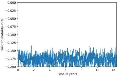
Appendix A illustrates the negative yield to maturity simulated sequence along with the corresponding zero coupon bond prices.

4.2

Simulated zero coupon bond VaR

In this section we illustrate the VaR computation of a simulated zero coupon bond using pulled-to-par returns.

Following the Basel recommendations [Basel II(2006)] we start to compute VaR one year after the beginning of our period of analysis so that the VaR is computed with a minimum of one year of historical data. Then, we compute VaR at each instant using all the available historical data until that instant.

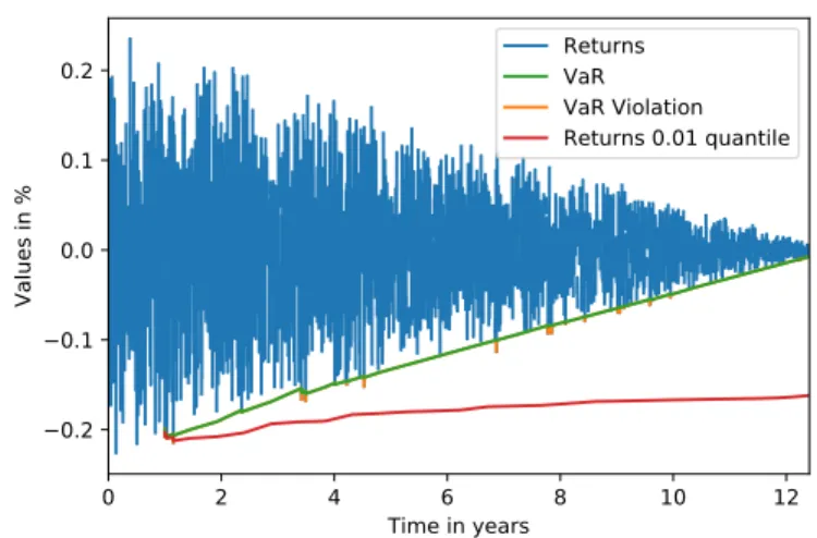
Figure 1 illustrates the historical returns and the VaR value obtained using the historical simulation method over the proposed pull-to-par returns, for the 12.8 maturity zero coupon bond whose prices are illustrated in Appendix A.

The horizon and confidence level is ∆ = 1 day andα= 0.99, respectively. The

returns that violate the VaR value are also showed.

It is clear from Figure 1 that the pulled-to-par VaR value follows the histor-ical returns pattern, diminishing towards zero as time to maturity approaches.

Just for illustration purposes Figure 1 also includes the 1−0.99 quantile of

the historical returns. It is clear from Figure 1 that this quantile can not be used to compute VaR. It does not follow the returns diminishing pattern. As a consequence there are almost no violations of this quantile which would result in an invalid VaR sequence.

In order to validate the obtained VaR sequences we applied both the stan-dard Bernoulli coverage test, for the level of VaR violations, and the text of [Christoffersen(1998)] for violations of independence. Implementation of both tests in several programming languages is provided in [Danelsson(2015)].

Table 1 shows both statistical tests p-values for the VaR sequence of Figure 1. Using the common p-value threshold of 0.05, it confirms that the Var sequence of Figure 1 is valid. The returns VaR violations in Figure 1 (orange excedences) of the pulled-to-par VaR (green line), occur as required at with 1% frequency and are independent.

(11)

0 2 4 6 8 10 12 Time in years 0.2 0.1 0.0 0.1 0.2 Values in % Returns VaR VaR Violation Returns 0.01 quantile

Figure 1: One day horizon, 0.99 confidence level, 12.8 maturity zero coupon bond pulled-to-par VaR example.

p-value

Level test 0.402

Independence test 0.414

Table 1: Figure 1 VaR violations statistical testsp-values.

4.3

VaR computation performance

The historical simulation method is based on the convergence of the empirical returns distribution to the real distribution. This convergence takes place as the number of returns tends to infinity. In practice the number of returns is limited. In this section we evaluate the performance of the pulled-to-par VaR computation, with pulled in the simulation scenario previously described.

Ideally we would consider the confidence levels from Basel recommendations, namely, 97.5% and 99% [Basel II(2006), Basel II(2016)], as well as the recom-mended 10 day time horizon. However, in terms of the time horizon, and since it also allowed shorter horizons to be scaled to the 10 days period, here e evaluate 1 day periods. This maximizes the number of returns available and allow for a better performance evaluation.

We repeat the VaR computation 1000 times for each confidence level. These number of repetitions was empirically determined by observing that the perfor-mance ratios remain almost unchanged around 500 repetitions. We just doubled this number and observed that the ratios did not change.

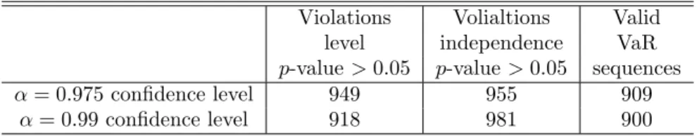
Table 2 illustrates the performance ratios obtained. Under the described simulation scenario the performance of the one day VaR computation for a

(12)

period slightly exceeding 10 years is always above 90%.

Violations Volialtions Valid

level independence VaR

p-value>0.05 p-value>0.05 sequences

α= 0.975 confidence level 949 955 909

α= 0.99 confidence level 918 981 900

Table 2: One day VaR computation performance over 1000 repetitions.

Figure 1 together with Table 2 summarize the overall idea of this paper. It is clear from Figure 1 that bond historical returns tend to zero as maturity approaches (blue line). This is the direct consequence of the pull-to-par con-vergence of bond prices to the par value at maturity. It is also clear that the quantile of the historical returns (red line) systematically overestimates VaR as there are almost no historical returns violations of this value. On the other hand, the pulled-to-par VaR value proposed (green line) is indeed adjusted for the pull-to-par pattern as it clearly follow the diminishing pattern of the histor-ical returns. Table 2 shows that the historhistor-ical returns violations of this value do confirm that it is a valid VaR sequence for over more than 90% of the simulation repetitions.

4.4

Computational overhead

Expression (5) implies recalculation of pulled-to-par returns of each timetVaR is

computed. This results in a computational overhead compared to the historical simulation of portfolios of stocks, where no (pull-to-par) adjustment is needed.

However the pulled to par returns for each timetcan be computed independently

of each other. This means that they can be parallelized. Given the current trend

of multicore GPU’s6 _{we anticipate that this overhead will easily overcome.}

5

Real data

In this section we apply the pulled-to-par VaR method to real zero coupon bonds traded in the market.

The long term zero coupon bond market is almost nonexistent compared to the huge market of long term coupon bonds. However, investment houses detach

coupons and principal from coupon bonds and trade STRIPS7_{independently of}

the original bonds. As these STRIPS have only one cash-flow, for all practical purposes, they are nothing but zero coupon bonds.

Our database contains sovereign eurozone STRIPS daily prices from 2006-01-03 to 2018-06-01. The eurozone is a natural region of choice has it allows

6_{As an example the NVIDEA GEFORCE GTX 1080 Ti GPU has 3584 computing cores.} 7_{Separate Trading of Registered Interest and Principal of Securities}

(13)

trading of STRIPS of different countries, with very different risk profiles, un-der the same currency. All the STRIPS were issued before 2006-01-03 and all were alive at 2018-06-01. The maturities range from 2018-06-01 to 2019-06-01. One year ahead of the last prices date. The choice of this near to maturity scenario was intentional. It provides the presence the vanishing returns near maturity. There are 19 STRIPS. Two from Germany, 3 from France, 7 from Italy, 1 from Belgium, 1 from Netherlands, 3 from Austria and 2 from Spain. A preliminary analysis allowed noticing that the STRIPS from the same country exhibited highly correlated price sequences. Almost indistinguishable. There-fore we kept only one STRIPS from each country. We choose the one with the shorter maturity. The list of the 7 STRIPS used is in Appendix B.

We use STRIPS both individually and in portfolios. The results are for 0.99 confidence level and 1 day horizon.

5.1

Individual STRIPS

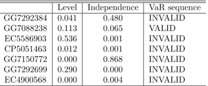
Table 3 shows level and independence VaR violations tests p-values for the

individual STRIPS. It can be observed a huge difference regarding our simula-tion scenario, where the stasimula-tionarity assumpsimula-tion was guaranteed. Given that the method proposed in this paper assumes that yields are stationary we at-tribute the generally poor performance of the method on real data to nonsta-tionary yields [Afonso et al.(2015)]. Nevertheless it should be highlighted that the analysis period includes a severe European sovereign debt crisis. Under this extremely adverse conditions there is one VaR valid sequence. Figure 2 shows the prices of this individual STRIPS and Figure 3 shows the corresponding re-turns, VaR sequence and VaR violations. For comparison purposes Figures 4 and 5 show the same sequences for and invalid VaR STRIPS.

Level Independence VaR sequence

GG7292384 0.041 0.480 INVALID GG7088238 0.113 0.065 VALID EC5586903 0.536 0.001 INVALID CP5051463 0.012 0.001 INVALID GG7150772 0.000 0.868 INVALID GG7292699 0.290 0.000 INVALID EC4900568 0.000 0.004 INVALID

Table 3: Level and independence VaR violations tests p-values of individual

STRIPS.

Comparing Figures 2 and 4, which illustrate a real bond price sequences, with Figure 7, which illustrates a simulated price sequence, a lack regularity in the evolution of the real bonds prices can be observed. This lack of regularity is characterized by high volatility periods mixed with small volatility periods as well as huge price drops (remarkably clear in Figure 4). This kind of evolution

(14)

2006 2008 2010 2012 2014 2016 2018 Years 60 65 70 75 80 85 90 95 100 Price in %

Figure 2: French GG7088238 STRIPS, 25-10-2018 maturity, historical prices.

2006 2008 2010 2012 2014 2016 2018 Years 2.0 1.5 1.0 0.5 0.0 0.5 1.0 1.5 2.0 Values in % Returns VaR VaR Violation

Figure 3: French GG7088238 STRIPS, 25-10-2018 maturity, one day horizon, 0.99 confidence level, returns, VaR and Var violations.

is a clear sign of nonstationarity of yields and compromises the results of the method application in a real data scenario.

This volatility pattern, can be observed again in Figures 3 and 5 reflected in the evolution of the historical returns. Instead of the smooth pattern of diminishing historical returns as maturity approaches, observed in Figure 1, the real data sequence exhibits periods of diminishing returns followed by periods of large returns.

(15)

2006 2008 2010 2012 2014 2016 2018 Years 60 70 80 90 100 Price in %

Figure 4: Italy EC5586903 STRIPS, 01-08-2018 maturity, historical prices.

2006 2008 2010 2012 2014 2016 2018 Years 4 3 2 1 0 1 2 3 4 Values in % Returns VaR VaR Violation

Figure 5: Italy EC5586903 STRIPS, 01-08-2018 maturity, one day horizon, 0.99 confidence level, returns, VaR and Var violations.

5, that the VaR value, computed we the proposed pull-to-par returns, is in fact adjusted to the pull-to-par diminishing pattern of the historical returns, leading to one valid VaR sequence. That of the French STRIPS GG7088238.

The overall conclusion of this discussion is that the stationarity assumption seems to be too strong for the real data scenario leading to a general poor performance in the case of individual STRIPS. Just one in the seven STRIPS tested resulted in a valid VaR sequence.

(16)

5.2

Portfolios

With the 7 STRIPS available we constructed all the possible portfolios with the number of STRIPS varying from 1 to 7 (the portfolios with 1 STRIPS equals the individual case described in the preceding section but are repeated here for means of comparison). Table 4 shows the number of valid portfolios VaR. Despite the poor general performance it can be observed that the diversification reached with portfolios with such a small number of portfolios allows the number of valid VaR sequences to increase.

Number of Number of STRIPS Number of Valid VaR

Portfolios per Portfolio Valid VaR Percentage

7 1 1 14% 21 2 5 24% 35 3 7 20% 35 4 8 23% 21 5 5 24% 7 6 2 29% 1 7 0 0%

Table 4: Number of valid Portfolios VaR sequences.

This can be observed right on the first two lines of Table 4, where the number of STRIPS in the portfolios was increased from 1 to 2. The percentage of valid VaR sequences in portfolios with just one STRIPS is 14%. But the percentage of valid VaR sequences in portfolios with two STRIPS increases to 24%. Given that the pulled-to-par VaR method requires stationary yields this increase can be explained by the contributions of the diversification to the portfolio stationarity yield.

6

Conclusions

In this paper we propose adjusting zero coupon bonds historical returns in such a way that allows VaR computation for portfolios, using the historical simulation

method. Thepulled-to-par VaR method.

We prove that the proposed VaR method leads to accurate VaR computa-tions whenever zero coupon bonds yields to maturity are stationary.

Simulation results show that one day VaR computation performance under Basel recommendations for a 10 years period is above 90%.

Real data performance on individual STRIPS is poor due the nonstationarity of bond rates in the period under analysis, [Afonso et al.(2015)]. Our sample

includes the European sovereign debt crisis of 2010-2014. Despite this, the

diversification effect in portfolios with a very small number of STRIPS, such as 3 and 4, do allow for increasing performance.

(17)

We identify the following strengths of the proposed method. The portfolio specific VaR is computed while using the market as the only source of informa-tion. The only information need is market prices. Neither subjective risk factors mapping [Alexander(2009)], risk factors correlations, standard maturities inter-polation, interest rate and credit risk separation, nor ratings, are needed.

Regarding weaknesses, the proposed method inherits all the known weak-nesses of the historical simulation method, namely, the need for stationary of the historical returns used (or adjusted historical returns in our case), and the need of large amounts of synchronized historical data for all securities in the portfolio, [McNeil, Frey and Embrechts(2005)].

Funding

Research was partially supported by Funded by CMA-UID/MAT/00297/2019 and CEMAPRE - UID/MULTI/00491/2019.

A

Simulation Example

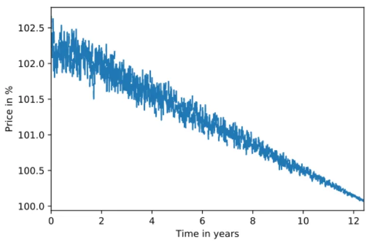
In this section we illustrate in Figure 6 a negative yield to maturity simulated sequence along with the corresponding zero coupon bond prices in Figure 7.

0 2 4 6 8 10 12 Time in years 0.200 0.175 0.150 0.125 0.100 0.075 0.050 0.025 0.000 Yield to maturity in %

(18)

0 2 4 6 8 10 12 Time in years 100.0 100.5 101.0 101.5 102.0 102.5 Price in %

Figure 7: 12.8 maturity zero coupon bond price sequence. The corresponding yields to maturity sequence is the one in Figure 6.

B

STRIPS list

Table 5: STRIPS Database.

Bloomberg ID Maturity Issuer Name

GG7292384 04-07-2018 Deutsche Bundesrepublik Coupon STRIPS

GG7088238 25-10-2018 French Republic Government Bond OAT Coupon STRIPS

EC5586903 01-08-2018 Italy Buoni Poliennali del Tesoro Coupon STRIPS

CP5051463 28-03-2019 Kingdom of Belgium Government Bond Coupon STRIPS

GG7150772 15-01-2019 Netherlands Government Bond Coupon STRIPS

GG7292699 15-07-2018 Republic of Austria Government Bond Coupon STRIPS

(19)

References

[Christoffersen(1998)] Christoffersen, P. F.: Evaluating interval forecasts.

In-ternational Economic Review,39(1998) 841862.

[Alexander(2009)] Alexander, C.: Market Risk Analysis, Value at Risk Models.

John Wiley & Sons, 2009.

[McNeil, Frey and Embrechts(2005)] McNeil, A.J. and Frey, R. and Embrechts, P.: Quantitative Risk Management: Concepts, Techniques, and Tools. Princeton University Press, 2005.

[Papoulis(1984)] Papoulis, A.: Probability, Random Variables, and Stochastic

Processes, Second Edition. McGraw-Hill, 1984.

[Dowd(2007)] Dowd, K.: Measuring market risk, Second Edition, p 84. John

Wiley & Sons, 2007.

[Abad, Benito and L´opez(2014)] Abad, P. and Benito, S. and L´opez, C.: A

comprehensive review of Value at Risk methodologies.The Spanish Review

of Financial Economics,12-115-32, Elsevier, 2014.

[Basel II(2006)] Basel Committee on Banking Supervision: International

Con-vergence of Capital Measurement and Capital Standards A Revised Frame-work Comprehensive Version. Bank for International Settlements, 2006.

[Basel II(2016)] Basel Committee on Banking Supervision:STANDARDS

Min-imum capital requirements for market risk. Bank for International Settle-ments, 2016.

[Mehta et al.(2012)] Mehta, A. and Neukirchen, M. and Pfetsch, S. and