Using graph structural information about flows to enhance short-term demand prediction in bike-sharing systems

(1)

Contents lists available atScienceDirect

Computers, Environment and Urban Systems

journal homepage:www.elsevier.com/locate/ceus

Using graph structural information about

ﬂ

ows to enhance short-term

demand prediction in bike-sharing systems

Yuanxuan Yang

a,b,⁎

, Alison Heppenstall

a

, Andy Turner

a

, Alexis Comber

a a_{School of Geography, University of Leeds, Leeds LS2 9JT, UK}

b_{Department of Geography and Planning, University of Liverpool, UK}

A R T I C L E I N F O Keywords: Bike-sharing Traﬃc prediction Graph theory Urban dynamics Sustainable transport A B S T R A C T

Short-term demand prediction is important for managing transportation infrastructure, particularly in times of disruption, or around new developments. Many bike-sharing schemes face the challenges of managing service provision and bikefleet rebalancing due to the“tidalflows”of travel and use. For them, it is crucial to have precise predictions of travel demand at afine spatiotemporal granularities. Despite recent advances in machine learning approaches (e.g. deep neural networks) and in short-term traffic demand predictions, relatively few studies have examined this issue using a feature engineering approach to inform model selection. This research extracts novel time-lagged variables describing graph structures andflow interactions from real-world bike usage datasets, including graph node Out-strength, In-strength, Out-degree, In-degree and PageRank. These are used as inputs to different machine learning algorithms to predict short-term bike demand. The results of the experiments indicate the graph-based attributes to be more important in demand prediction than more com-monly used meteorological information. The results from the different machine learning approaches (XGBoost, MLP, LSTM) improve when time-lagged graph information is included. Deep neural networks were found to be better able to handle the sequences of the time-lagged graph variables than other approaches, resulting in more accurate forecasting. Thus incorporating graph-based features can improve understanding and modelling of demand patterns in urban areas, supporting bike-sharing schemes and promoting sustainable transport. The proposed approach can be extended into many existing models using spatial data and can be readily transferred to other applications for predicting dynamics in mass transit systems. A number of limitations and areas of further work are discussed.

1. Introduction

Research has shown that bike-sharing contributes to improved air quality and reduced congestion in cities as a part of a sustainable travel infrastructure (Lovelace & Philips, 2014;Shaheen, Guzman, & Zhang, 2010). Its global popularity has increased in the last few years due to advantages in both cost and convenience over other forms of transport such as cars. A growing number of cities have operated such schemes to promote sustainable mobility, such as Santander Bikes (London), Citi Bikes (New York) and more advanced dock-less systems (e.g. Mobike in Chinese cities). Bike-sharing schemes provide a key component of urban transportation infrastructures by providing an “extension ser-vice”for the“ﬁrst/last mile”from other public transport hubs (Ma, Liu, & Erdoğan, 2015; Saberi, Ghamami, Gu, Shojaei, & Fishman, 2018; Shaheen et al., 2010).

While bike-sharing greatly enhances urban mobility as an aﬀordable

and sustainable traffic mode (Fishman, 2016), meeting the demand of users poses a challenge to scheme operators. This is due to the“tidal flows” of bike-sharing trips, with certain areas in the city facing the problem of insufficient bikes (Beecham, Wood, & Bowerman, 2014). For example, during the morning rush hour, the number of commuting trips departing from residential areas will be high, potentially leading to a deficit of available bikes in those areas. This results in reduced service reliability and reduced user satisfaction (Fishman, 2016; O'Brien, Cheshire, & Batty, 2014). Accurate and up-to-date estimations of travel demands across the city over the course of the day are crucial for successful bike scheme management andfleet rebalancing. This also has attracted a lot of research interest in recent years.

Researchers have used a combination of statistical models, machine learning and more recently, deep learning neural networks to forecast short-term travel demands (Karlaftis & Vlahogianni, 2011;Lin, He, & Peeta, 2018; Vlahogianni, Karlaftis, & Golias, 2014). While some

https://doi.org/10.1016/j.compenvurbsys.2020.101521

Received 8 January 2020; Received in revised form 25 June 2020; Accepted 26 June 2020 ⁎_{Corresponding author}

E-mail address:[email protected](Y. Yang).

(2)

studies have evaluated alternative predictive models for demand fore-casting, fewer studies have focused on feature engineering, i.e. the identification and extraction of latent data features that can potentially improve the performance of predictive models (Borges et al., 2017). Recent thinking conceptualises cities as complex systems driven by the pattern offlows and networks of relations (Batty, 2013). One approach to understanding the temporality of urban dynamics and transportation flows is through the analysis of graph structures (Hoang, Zheng, & Singh, 2016;Lin et al., 2018;Yao et al., 2018), which has been shown to support insights into different urban and transport problems. How-ever, as yet little research has been undertaken that examines how in-formation from temporal graphs can contribute to better traffic pre-diction in bike-sharing systems.

This paper evaluates the use of temporal information encoded in graph structures of bike trafficflow interactions for forecasting short-term bike-sharing demand. The experiments in this work retained in-itial model hyper-parameters to demonstrate the utility of the graph derived features.Section 2 introduces related work and reviews dif-ferent models and inputs used for predicting bike travel demand. Section 3presents the data and the concept of graph-based measures in the transportation network. It compares graph-based features to other commonly used variables such as meteorological data, in terms of im-portance, explanatory power and their potential contribution to de-mand prediction models.Section 4presents and compares the results in detail and describes the relative benefits of including graph-based fea-tures for improved forecasting. The feafea-tures, methods and their ap-plicability to other application domains related to transport andflow predictions are discussed and conclusions are drawn (Section 5). 2. Related works

There are two conventional approaches for dealing with dock-based bike-sharing travel demand forecasting problems: predicting at an in-dividual station level or over aggregated groups / areas. The former approach models dynamics at each station (Lin et al., 2018), while the latter focuses on regional dynamics (Xu, Ying, Wu, & Lin, 2013;Zhou et al., 2019). Station level modelling can support bike-fleet manage-ment atfiner spatial granularities, but can be less accurate due to higher levels of noise in the data. Many studies (Li, Zheng, Zhang, & Chen, 2015; Zhou, Li, et al., 2019) attempt to predict demand over small geographical areas for the following reasons. Firstly, bike docking sta-tions are dynamic in urban areas over long periods. New stasta-tions may be added, with existing stations removed, or relocated. Analysing small clusters of stations allows local travel dynamics to be captured and supports a deeper understanding of these dynamics (Li et al., 2015; Zhou, Li, et al., 2019). Secondly, the emergence and rise of dockless bike-sharing may change the nature of bike-sharing in the future. Dockless schemes allow individuals to borrow and return bikes at any location, rather than at fixed docking stations, this makes it both challenging as well as important to understand travel demand at the small area level (Cao & Shen, 2019; Yang, Heppenstall, Turner, & Comber, 2019). Finally, grouping stations into small area-based clusters supports bike fleet management regardless of the scheme type, with sufficient spatial grain to support rebalancing (Li et al., 2015).

A broad range of data-driven models have been proposed to forecast short-term travel demand in bike-sharing systems and other transpor-tation systems such as the metro, buses and taxis (Vlahogianni et al., 2014). These can be categorised into parametric statistical models, and nonparametric machine learning (ML) approaches (Zhang, Cheng, & Ren, 2019). Some examples of the former group include ARIMA (Au-toregressive Integrated Moving Average model) and its variants (e.g. ARIMAX, seasonal ARIMA) and Bayesian Networks (Froehlich, Neumann, & Oliver, 2009). Statistical models are easier to interpret but may have lower prediction accuracies when compared to ML models. Karlaftis and Vlahogianni (2011)observed a trend of research moving from statistical models to ML models as a result of both increased data

accessibility and computing power.

Different ML models have been applied to forecast short-term traffic demand, such as support vector regression (Xu et al., 2013) and Re-gression Trees (Li et al., 2015). More recently, deep neural networks have attracted significant research interest due to their automatic fea-ture extraction capacity and their success in handling temporal, spatial and semantic dependencies.

Temporal dependencies include snapshots of historical relation-ships, and have been widely used for traﬃc demand prediction pro-blems (Froehlich et al., 2009;Giot & Cherrier, 2014;Li & Shuai, 2018). For example, useful travel demand information is retained from the last few hours to suggest demand intensity trends. Deep neural networks such as Recurrent Neural Networks (RNNs) provide powerful tools for dealing with sequential information, and are suitable for analysing temporal dependencies. These recurrently connect hidden layers with diﬀerent timestamps, identifying sequential characteristics and patterns that are then used to predict the next likely scenario. LSTM (Long Short-Term Memory) and GRU (Gated Recurrent Unit) Networks, both en-hanced forms of RNNs, have been used to predict travel demand (Fu, Zhang, & Li, 2016;Xu, Ji, & Liu, 2018). They are able to overcome the “vanishing gradients”problem common in neural networks. This occurs when gradients of the loss function approach zero, making the neural network hard to train, which commonly happens when processing long-term temporal dependencies with standard RNNs.

The idea of spatial dependencies (Tobler, 1970) suggests that in-formation from nearby locations can contribute to improved fore-casting. Some studies (Ke, Zheng, Yang, & Chen, 2017) have applied Convolutional Neural Networks (CNNs) to capture spatial dependencies in traffic demand forecasting. CNNs were initially designed for the analysis of gridded data, such as images. They capture spatial de-pendencies between grid locations using localised filters or kernels. Previous research (Ke et al., 2017;Zhang, Zheng, & Qi, 2017) using this approach to analyse travel demand divided urban areas into two-di-mensional grid cells and calculated the demand across each grid, with demand intensity represented as colour scales. However, the selection of grid size is critical and difficult to determine objectively: if the grid is too coarse, it will fail to capture sufficient spatial granularity to support bikefleet management. If it is toofine, then the computational burden increases significantly due to the large image-like matrices containing redundant information (grid cells with zero demand).

More recent studies have used semantic dependence. Semantically similar areas may not be contiguous or near each other. For example, bike stations located in two distant residential areas may have similar temporal patterns of travel demand. Characterising semantic de-pendencies from such similar areas may improve model performance. Some research has quantified the similarity of historical travel demand sequences over different sites and constructed semantic graphs to connect similar places (Hoang et al., 2016;Yao, Wu, et al., 2018).Lin et al. (2018) applied Multi-Graph Convolutional Neural Networks (MGCNN) to capture pairwise relations between bike stations, using spatial and semantic graphs to provide multi-graph embedding. How-ever, the pre-processing requirements of capturing demand sequence similarities for MGCNNs are heavy, requiring at least one year's his-torical data to obtain a good prediction accuracy in bike demand forecasting (Chai, Wang, & Yang, 2018;Lin et al., 2018). This leads to limitations for analyses of sites and systems with insufficient historical travel records, for example, when new service stations or areas are introduced into a bike-sharing scheme.

Outside of the deep neural networks family, XGBoost (Chen & Guestrin, 2016), an implementation of gradient boosted decision/re-gression trees, has been found to perform well in transport prediction problems and was the winner of the Kaggle bike-sharing prediction competition (Kaggle, 2015). Some research compared XGBoost to neural networks (Lin et al., 2018; Ma, Guo, Guo, & Guo, 2019;Yao, Tang, Wei, Zheng, & Li, 2019;Yao, Wu, et al., 2018;Zhou et al., 2019), and most of these suggest that XGBoost is capable of obtaining better or

(3)

similar performances in travel demand forecasting when compared to RNNs (LSTM, GRU), CNNs and to hybrid neural networks, for example ConvLSTM (convolutional LSTM), ST-ResNet (Deep Spatio-Temporal Residual Network). XGBoost is also found to have comparable perfor-mance to MGCNN in the work ofZhou, Chen, et al. (2019), in 50% of datasets XGBoost produced better predictions than MGCNN. However, XGBoost may be inferior to some state-of-the-art fusion deep neural networks, such as Spatio-Temporal U-shape Networks (Zhou, Chen, et al., 2019) and Spatial-Temporal Dynamic Networks (Yao et al., 2018).

Despite the intense competition among complex algorithms, whe-ther one model outperforms the owhe-thers is questionable. Li et al. (2019) compared various models for traffic demand forecasting, and concluded that a universally best model does not exist. When considering different specific areas and timestamps, several algorithms (e.g. LSTM and XGBoost) may offer better solutions depending on the nature of the spatial and temporal variables. Therefore, it could be beneficial to combine the prediction results of different models (KDD-Cup, 2017). There are also reproducibility issues in the literature; for example, ST-ResNet was found to outperform XGBoost inChen et al. (2018). How-ever, some studies (Ma et al., 2019;Yao et al., 2019) show contrasting results. MGCNN shows advances in predicting dynamics in planar-networks (e.g. road planar-networks) that have a clear concept of graph con-struction. However, for non-planar networks such as origin and desti-nation graphs (e.g. bike-sharing graph), the nodes (docking stations) connection is subject to several factors including time-series similarity and distance to each other, etc. They rely on an arbitrary and ambig-uous choice of threshold (e.g. proximity, similarity, consistency); as well as specific preprocessing (e.g. removing less-used stations) (Chai et al., 2018;Lin et al., 2018). These lead to reproducibility issue to some extent. For example,Zhou, Chen, et al. (2019)found that MGCNN is worse than Xgboost on several datasets, whileLin et al. (2018) sug-gested a better performance on New York bike-sharing. Differences in results may be due to the complexity of hyperparameter tuning in deep neural networks, varied model performance on different datasets, dif-ferent preprocessing or unfair comparisons (Karlaftis & Vlahogianni, 2011). This makes the“best”models even more of a challnge to iden-tify.

Overall, short-term traffic forecasting is a highly dynamic and de-veloping research arena with ever-growing literature that has mainly focused on testing and comparing the performance of alternative models (Vlahogianni et al., 2014). This focus on models has left other vital questions relatively unaddressed, for example, consideration of what kinds of variables should be included in models. The performance of a predictive model is not only associated with its generalisation ability but also its dependency on the input data and features (Hall & Smith, 1998). Deep learning neural networks require less effort to manually extract features from raw data (Goodfellow, Bengio, & Courville, 2016;Lin et al., 2018), but still may benefit from effective feature engineering, especially when the size of the training dataset is limited (Ketkar, 2017). Research has suggested that short-term traffic demand can be inferred from its spatiotemporal properties (e.g. his-torical travel demand) but may also benefit from other explanatory variables (Ke et al., 2017). However, there is only limited insight into the nature and direction of feature engineering, with studies generally using temporal features (e.g. time of day, day of the week) and me-teorological features (e.g. temperature) to forecast travel demand (Giot & Cherrier, 2014; Lin et al., 2018; Salaken, Hosen, Khosravi, & Nahavandi, 2015). For example, the work ofYang et al. (2016)suggests that average trips amount on weekdays are relatively smaller than during weekends (with the patterns being opposite for stations in re-sidential areas). Both day of week and calendar events (Kim, 2018) are informative for modelling trip demand. Meteorological factors have a huge influence on user behaviours in bike-sharing systems, and good weather is strongly correlated with higher trip amount (Kim, 2018; Yang et al., 2016). In particular, temperature has been included in

many studies and identified as a useful feature for predicting bike trip demand in various cities and regions (e.g. American, Asian, Europe) under different climates and cultural backgrounds (Rudloff& Lackner, 2013;Li et al., 2015;Salaken et al., 2015; Yang et al., 2016). Some studies have also used urban context such as land-use, Points of Interest (POI) (Tran, Ovtracht, & D'arcier, 2015;Xu et al., 2018) and event in-formation (e.g. metro delays, concerts) (Chen et al., 2016;Rodrigues, Markou, & Pereira, 2019) to improve forecasts. The work ofXu et al. (2018)suggests that land-use information derived from POI is not as helpful as meteorological features, but still can enhance prediction performance for neural network models. However, these are data en-richment approaches, requiring data from other sources (e.g. POI, textual data from twitter), some of which are relatively difficult to obtain, process and merge into models. This leaves an important question: is it possible to derive additional useful information from the flow data itself, such as bike travel records, to improve the prediction performance further? In machine learning, feature engineering is the process of using domain knowledge to extract and transform raw data into explanatory features. The result is that ML algorithms are better able to detect patterns in input data, leading to better outcomes. As yet relatively little research has been undertaken using such approaches in this area to consider what features can be derived from raw travel data using domain knowledge, and whether they can improve different traffic prediction models. Here we examine the graph structures present in bike travel records.

Research using graph theory has been successfully applied to ana-lyse urban phenomena such as polycentric transformation, urban resi-lience, infrastructure updates and mobility change to analyse and un-derstand urbanflows such as travel (Batty, 2013; Yang et al., 2019; Zhong, Arisona, Huang, Batty, & Schmitt, 2014). Graph structures of travelflow spatial and temporal patterns may be used for interpreting urban dynamics as well for traffic demand prediction (Zhang et al., 2017).Austwick, O'Brien, Strano, and Viana (2013) examined bike-sharing systems in different cities. They highlighted the use of graph analysis for understanding urban flow in spatial systems and whilst Zhang et al. (2017)argued that the historical regional inflows are re-lated to outflows. Generally, studies examining short-term traffic de-mand forecasting have not fully exploited inflow interactions. The current state of the art in this area uses historical demand and common environmental variables (e.g. temperature) to predict future demand (Feng, Chen, Du, Li, & Jing, 2018;Li et al., 2015;Li & Axhausen, 2019; Li & Shuai, 2018;Lin et al., 2018;Xu et al., 2013;Yao, Wu, et al., 2018). There are many kinds of graph information (e.g. degree, PageRank) that can be derived from bike travel data to describeflow interactions and to characterise the different urban places within the graph, for example, to infer the likelihoods of bike trips starting from specific regions. The utility of spatio-temporal graph properties to support short-term bike-sharing demand prediction has not been evaluated, and the research described in this paper starts to address this.

3. Methods

3.1. Study area and data

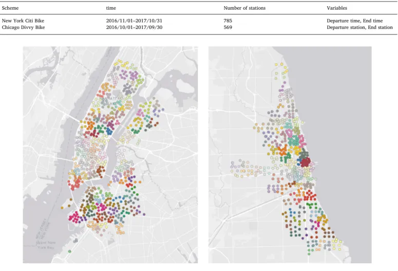
This study uses dock-based bike-sharing data from two cities to ensure theﬁndings are not exclusive to a speciﬁc case. They are New York Citi bike and Chicago Divvy bike schemes, as shown inTable 1. The datasets cover one year and contain variables describing bike trip departure and end time, departure station and end station. Corre-sponding hourly meteorological data were obtained from open weather map (https://openweathermap.org/), and the variables included tem-perature, humidity, wind speed, pressure and weather description (e.g. Cloudy, light rain).

(4)

3.2. Data pre-processing 3.2.1. Station groups

This study predicts regional (small area) demand and groups of stations based on their spatial proximity. A hierarchical clustering method was applied to cluster stations into 120 and 80 groups in the New York and Chicago data, respectively. The choice of kclusters is arbitrary and usually depends on the knowledge of the study area (Li et al., 2015). Here, values ofkwere chosen to generate groups con-sisting of roughly 6 or 7 stations on average (Table 1shows total station number).Fig. 1(a, b) shows the groups of stations (small areas), where the shading and plot characters indicate diﬀerent clusters.

3.2.2. Travelﬂow graph structure construction

Graph theory is a mathematical approach for modelling pairwise relations between individuals. A graph structure typically consists of observations represented by nodes or vertices and their relationships represented by links or edges (although this can be reversed). A system formed of nodes and links that are interconnected is termed a graph. In urban and transport studies, public transportation systems have been viewed as complex networks (Saberi et al., 2018; Yang et al., 2019; Zhong et al., 2014) and represented as graphs in order to generate diﬀerent scale-free graph-based measures pertaining to the network.

Generally, transportation hubs and urban areas are regarded as graph nodes, and the travelﬂows between a pair of nodes generate links to connect them. Analysis of the networkﬂows between nodes and their changes, for example over time, provides insights into spatiotemporal mobility characteristics in transportation systems.Saberi et al. (2018) used graph-based analysis to examine the impact of public transit dis-ruptions on bike-sharing usage and travel behaviours.

In this study, hourly graph structures were constructed from bike trip records. Each group of bike stations were cast as node, and the volume of hourly bike trips between any two nodes was used to gen-erate edges to represent the origin-destination ﬂows between them. This resulted in a series of temporally weighted and directed graph structures, from which a number of graph properties were calculated, describing the state of each node at diﬀerent times. FollowingZhong et al. (2014);Saberi et al. (2018);Yang et al. (2019), the graph prop-erties were:

(1) Strength–the total of the edge weights. In a directed and weighted graph structure, there are two strength measures, in-strength and out-strength. Here they represent the number of trips that end at and start from a node in the network. Out-strength can also be in-terpreted as the number of departures–i.e. travel demand. (2) Degree – the number of edges that are incidental to the node, Table 1

Bike-sharing data.

Scheme time Number of stations Variables

New York Citi Bike 2016/11/01–2017/10/31 785 Departure time, End time

Chicago Divvy Bike 2016/10/01–2017/09/30 569 Departure station, End station

(5)

indicating the number of neighbouring nodes. In-degree and out-degree account for the number of in-ﬂow and out-ﬂow links in a directed graph. A node is considered important if it is connected to many neighbours, and for urban mobility networks, the degree can be used to describe the connectivity and accessibility to destinations or activities across the network (Zhong et al., 2014).

(3) PageRank – a measure of node importance. This was ﬁrst in-troduced by Google to evaluate the importance of a web page (Brin & Page, 1998). The key idea behind PageRank in a graph context is that nodes with the same degree may not have the same importance in a graph. By not counting links from other nodes equally, Pa-geRank treats an edge from a strongly connected node as more important than an edge linked to a node with few connections. Assume graph nodeA has incoming edgesT1…Tn, and the

para-meterdis a damping factor (0.85 as the default value),C(Tn)is

deﬁned as the out-degree of nodeTn. The PageRank (PR) of a node Ais denoted as follows: ⎜ ⎟ = − + ⎛ ⎝ +⋯+ ⎞ ⎠ PR A d d PR T C T PR T C T ( ) (1 ) ( ) ( ) ( ) ( ) n n 1 1 (1)

The PageRank of nodeAcan thus be calculated using an iterative algorithm that corresponds to the principal eigenvector of the nor-malised link matrix of the graph (Brin & Page, 1998). Note that the PageRank forms a probability distribution over graph nodes, so that the sum of all nodes' PageRanks will be one. PageRank is an additional indicator of relative node importance and centrality in a graph. In a transportation network, PageRank can help to identify key nodes (places) in the system that have a high impact on transportation eﬃ -ciency.

(4) Betweenness–the number of links that pass through a node. The greater the betweenness the more important it is (Newman, 2005). For each pair of nodes in a graph, there exists at least one shortest path between them. Node betweenness refers to the number of the shortest paths that pass through a node. Betweenness represents the extent to which nodes are connected, and indicate transfers from one area to another in a transport system. Although bike-sharing trips generally do not rely on or are impacted by middle stations to reach the destination, they are still limited by station availabilities (available bike and empty docks) to start or complete journeys. The work ofSaberi et al. (2018)suggests that in bike-sharing systems, the probability and spatial distribution of betweenness changed in response to urban public transit failure. Furthermore, betweenness is helpful to examine system changes during special events and adverse weather conditions.

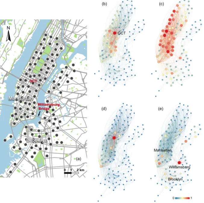
Fig. 2 (a) shows the map of the New York bike-sharing station groups, with each dot indicating the group's central position.Fig. 2 (b-e) give examples of the graph information properties for each node, with the different properties normalised to [0,1] for visualization pur-poses. The redder and larger the plot character, the higher value it has. This graph was constructed using 1 h (8,00 to 9:00 am on October 25, 2017) of bike-sharing travel data, which representsflow interactions in the morning rush hour.Fig. 2(b) shows the out-strength, directly re-presenting area travel demand intensities. Areas close to Grand Central Terminal (GCT) have the most bike trips with high numbers of trips in surrounding areas (Midtown Manhattan).Fig. 2(c) illustrates the dis-tribution of out-degree, and suggests that different regions in Man-hattan all have high levels offlow interactions indicated by the number of neighbours linked by travelflows. Interestingly, the GCT region does not have the highest out-degree. This is because the trip destinations are less diverse during the selected period.Fig. 2(d) shows the PageRank and has a similar pattern toFig. 2(b), emphasising the importance of GCT in the network.Fig. 2(e), shows that betweenness has a different spatial pattern to the other figures (Fig. 2b, c, d). It highlights the

region of Williamsburg, located at the east side of the Williamsburg bridge. The high betweenness value indicates its crucial role as a bridge in the graph connecting different parts of the city (e.g. Manhattan and Brooklyn). The different graph properties describe theflows and their interactions in the graph structure, allow the importance of each node to be characterized in different ways.

3.3. Analysis

3.3.1. Feature importance

Various models can be used to evaluate feature importance for making predictions, for example, Random Forest and Support Vector Machine. Among these approaches, XGBoost (extreme gradient boosting) is a gradient boosted regression tree algorithm and has been found to be one of the most powerful models in the literature (Li & Axhausen, 2019;Lin et al., 2018) and in competitions (Kaggle, 2015; KDD-Cup, 2017) to predict bike-sharing travels. It has been shown to have a comparable (or better) performance to several advanced deep neural networks such as ST-ResNet (Ma et al., 2019;Yao et al., 2019; Zhou, Chen, et al., 2019). Another advantage of XGBoost is that its results are easily explainable: once the boosted trees are constructed, importance (i.e. gain) scores of each feature can readily be retrieved. The importance metric provides an evaluation of how useful or valuable each feature is, based on the degree to which a feature is used to make key decisions in trees. Therefore, this study used XGBoost to evaluate feature importance.

There are potential multi-collinearity problems that may impact the feature importance identified from different models. Strong collinearity can affect model reliability and precision (Comber et al., 2018) and can result in unstable estimates of feature importance and therefore in-ferential and prediction biases (Dormann et al., 2013). As a result, model extrapolation may be erroneous, and there may be problems in separating variable effects (Meloun, Militký, Hill, & Brereton, 2002). For example, in a random forest model, the importance of a feature may be diluted by another highly correlated variable, because each tree is independent of others and random choice will be made on features. XGBoost has been found to be relatively immune to the multi-colli-nearity problem (Chen & Guestrin, 2016;Chen, Tong, Benesty, & Tang, 2018) because the algorithm does not re-focus on any specific link between feature and outcome after it has been made and learnt in the boosting process.

Table 2lists the input variables in the XGBoost model used to pre-dict bike-sharing demand. Based on the literature reviewed, temporal and meteorological variables were included in the Basic Features group (Li et al., 2015; Zhou, Chen, et al., 2019). Bike travel ﬂows were transformed into directed weighted graphs, allowing the strength and degree properties to represent theﬂow directions. Time-lagged travel demand is identical to time-lagged out-strength. All time-lagged prop-erties were obtained from the last hour to provide temporal dependence for the prediction (longer time-lags are examined inSections 4.2 and 4.3). As XGBoost only accepts numeric values, categorical variables (e.g. hour of day) were processed using Multiple Correspondence Analysis (Meng et al., 2016) to generate lower-dimensional numeric representations.

3.3.2. Adding time and graph information

A good feature is one that improves model performance (e.g. pre-diction) as it allows more parsimonious (less complex) models to be constructed, and non-optimised model hyperparameters to be included, whilst still generating good results. By continually adding diﬀerent features into a machine learning model, changes in prediction results can be evaluated accordingly. A good feature will reduce forecasting errors, while bad features will result in higher errors (and more noise). In this study, Multi-Layer Perceptron (MLP) neural networks were constructed to conﬁrm the usefulness of various input features. MLP is a class of feed-forward neural networks. It utilises backpropagation for

(6)

training, and its multiple layers and non-linear nature contribute to its ability to distinguish data that is not linearly separable. As a neural network, it has a relatively simple structure making it easier to con-struct and train than others. MLP also has been shown to have a strong performance in predicting short-term traﬃc demand (Li & Axhausen, 2019;Lin et al., 2018).

This studyfirstly constructed an MLP that is neither under- nor over-fitted, using the“Basic Features”listed inTable 2of meteorological and temporal features that included time-lagged travel demand of−1 h. Different time-lagged travel demand variables and graph information

properties were then sequentially added into the MLP, with the outputs evaluated accordingly. This identiﬁes which lagged-time steps are more strongly associated with current travel demand and also provides va-lidation of the important features as identiﬁed by the XGBoost.

An investigation of the hyperparameters determined that an MLP with two layers of 32 and 8 units neither under- or over-ﬁtted models on both datasets. The mini-batch size was set to 1024 and training epochs to 150 (enough for convergence). The loss function used was RMSE (Root Mean Square Error), which is denoted as

Fig. 2.An example of the spatial distribution of graph properties using 1 h of data, (a) station groups in New York, (b) out-strength, (c) out-degree, (d) PageRank, (e) betweenness.

Table 2

Variables in XGBoost.

Feature origin Feature type Variable

Basic Features Temporal Hour of day, Day of week, Holiday, Time-lagged travel demand (−1 h). Meteorological Temperature, Humidity, Wind speed, Weather description, Pressure. Graph features Time lagged (−1 h) graph information Out-strength, In-strength, Out-degree, In-degree, PageRank, Betweenness.

(7)

∑

= − = n A F RMSE 1 ( ) i n i i 1 2 (2) whereAiandFi are the actual value and forecast value respectively.

There are alternative loss functions, such as Mean Absolute Error (MAE), which may be used for training machine learning models. However, the errors are squared before being averaged in RMSE, thereby giving relatively high weight to large errors. RMSE was used in this study due to the fact that in a bike-sharing system, large errors of demand estimation may pose significant difficulties to scheme opera-tors for successful bikefleet rebalancing.

4. Results

4.1. Feature importance and variable selection

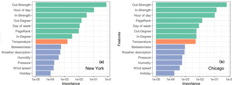
The data was split into training, validation and test datasets, with the data ordered by time. Thefirst 80% of records were assigned as the training set, the following 10% as validation and thefinal 10% as the test set. The training datasets were inputted to the XGBoost models to rank the importance of different features with the results are shown in Fig. 3. Generally, temperature is considered as an important factor re-lated to cycling activity (Miranda-Moreno & Nosal, 2011; Thomas, Jaarsma, & Tutert, 2013) and many bike travel demand prediction studies include temperature or a series of time-lagged temperatures as model inputs (Salaken et al., 2015; Zhou, Chen, et al., 2019). Inter-estingly here, in both case studies (Fig. 3a, b), out-strength, in-strength, out-degree, in-degree and PageRank were all found have greater (or comparable) importance scores than temperature, indicating their po-tential utility in short-term demand prediction. This suggests that de-spite temperature being widely used for bike-sharing demand predic-tion studies, several graph features are potentially more important. Betweenness failed to outperform temperature, probably due to it being less associated with travel demand intensity. As observed in Fig. 2, strength, degree and PageRank are relatively similar in their spatial patterns, while betweenness is different as it describes the“bridge ef-fect”of a node.

In summary, feature selection using an initial XGBoost model identiﬁed the following features for inclusion in subsequent models: out-strength (OS), in-strength (IS), out-degree (OD), in-degree (ID) and PageRank (PR). In the following section, the results of applying a dif-ferent machine learning model (MLP) are described to conﬁrm the utility of these graph information properties in solving bike-sharing demand prediction problems.

4.2. Adding time and graph information comparison

Two types of MLP were constructed in the experiment, namely MLP-GI and MLP-DT. The former requires that graph information (MLP-GI) properties at a time lag of−1 h are sequentially added into the model, with the order of out-strength (OS), in-strength in (IS), out-degree (OD), PageRank (PR) and in-degree (ID), as suggested inFig. 4(a). The MLP-DT model used time-lagged travel demand (MLP-DT) from only−1 h to a group of−1 to−5 h. This is a common approach, using multiple time-lagged demands from the last few hours provides a greater indication of temporal dependence in the models (Ke et al., 2017;Lin et al., 2018). Fig. 4shows box plots of the distribution of the RMSE of 15 ex-periments, with the results evaluated on the validation set. Initially, the two models (MLP-GI and MLP-DT) are identical because they both used the travel demand (i.e. out-strength) number from the last hour. As more variables included, the MLP-GI models benefit from additional lagged graph information, with decreasing RMSE, in both average and median values. This is observed in both datasets (Fig. 4a, b). Another finding is that adding OD (out-degree) and ID (in-degree) reduces prediction errors for the New York dataset (Fig. 4a), but has less effect with the Chicago data (Fig. 4b). The pattern accords with the previous finding inFig. 3, where OD and ID much outperform the benchmark (temperature) in the New York (Fig. 3 a), this again confirms the variable importance identified by XGBoost inSection 4.1.

In the MLP-DT groups, there is a diﬀerent pattern to MLP-GI. Although adding more time-lagged travel demand variables reduces errors initially, this improvement is reversed with longer sequences. In the case of New York (Fig. 4 a), the RMSE slightly increased after adding the travel demand of−5 h. For the Chicago data (Fig. 4b), the model shows underperformance after adding demand intensity of−4 h, with a higher mean and median RMSE.

The possible underperformance with a longer temporal dependence is a general phenomenon, observed and discussed in many studies (Ke et al., 2017). The performance does not always improve, when a long sequence of previous observations are fed into machine learning ap-proaches for modelling temporal dependency. The inclusion of in-formation at less correlated timestamps can lead to poor forecasting. Therefore, the majority of previous studies only chose speciﬁc time steps to provide temporal dependence and to predict travel demand (Ke et al., 2017;Lin et al., 2018).

Comparing MLP-GI and MLP-DT with the same number of extra variables, MLP-GI always outperforms MLP-DT (seeFig. 4). The pattern indicates that using the groups of graph information properties is more eﬀective than only using time-lagged observation of forecasting target (travel demand).

(8)

In summary, temporal dependence modelling is limited if only historical travel demand is utilised, because only a ﬁnite number of time lags will improve the prediction. However, better forecasting re-sults may be obtained by introducing graph information properties.

4.3. Model comparison

The analysis and results from the previous sections indicate the potential usefulness of information derived from the bike ﬂow inter-action graph, but the graph properties were all derived from a single lagged timestep. This section examines how diﬀerent ML models can comprehensively use varying lagged time-sequences of graph features and compares their performance with two other baseline approaches: HA (Historical Average) and ARIMA (Autoregressive Integrated Moving Average). The models are described as follows:

(1) HA: uses the historical average demand for prediction. For example, the travel demand of Tuesday 12:00 is predicted as the average value of all past Tuesday's at 12:00 in the training dataset. (2) ARIMA: a statistical model, ARIMA is commonly used for analysing

and forecasting time-series data. It has been widely applied in traffic prediction problems (Van Der Voort, Dougherty, & Watson, 1996;Williams & Hoel, 2003). In this work to predict demand at time T, the inputs to ARIMA were the demand observations from the first hour until T-1. It was undertaken using the automatic ARIMA model provided by the“forecast”package in R, a variation of the Hyndman-Khandakar algorithms (Hyndman et al., 2018). The model combines unit root tests, minimisation of the Akaike Information Criteria and Maximum Likelihood Estimation to con-struct the ARIMA. It should also be noted that the performance can be significantly influenced by model tuning, and there are also several variants such as seasonal ARIMA, which may generate better results.

(3) XGBoost: all features, including meteorological features, temporal features, and diﬀerent groups of time-lagged graph information features are placed into a one-dimensional vector and used for prediction.

(4) MLP: uses the same features as XGBoost, and like XGBoost, MLP does not diﬀerentiate between variables across time to model

temporal dependencies.

(5) LSTM: (Long-short Term Memory) is an improved version of RNN. Time-lagged variables are reshaped to a sequence and put into a bi-directional LSTM layer. Other temporal features (hour of day, day of week, holiday) and meteorological features are placed into a vector and processed using a densely-connected layer which is concatenated to the LSTM layer. The two branches are merged using another densely-connected layer. The LSTM unit is composed of three gates: input, forget and output gates. These gates determine whether to include new inputs, delete information and whether the hidden state of the current time step is carried over to the next time step (iteration). As a result, LSTMs suﬀer less from the vanishing gradients problem and can handle complex temporal dependencies. XGBoost, MLP, and LSTM models have three variants, denoted as “-TD”,”-PGI”,”-FGI” respectively. They all use the basic features in-cluding meteorological and temporal variables, but have diﬀerent in-puts in terms of graph information features.

(1) TD: uses time-lagged travel demand (out-strength) for prediction, as commonly observed in the literature (Lin et al., 2018).

(2) PGI: this uses part of the time-lagged graph information. Out-strength and in-Out-strength are provided for temporal dependence modelling and demand forecasting.

(3) FGI: uses the full set of time-lagged graph information properties that were identiﬁed as more important than the baseline tempera-ture variable; out-strength, in-strength, out-degree, in-degree in and PageRank.

Models with the same suﬃx (e.g. -PGI) used identical input features for travel demand prediction.

Incorporating the flexibility of feature engineering in machine learning models, allows them to achieve better results under the same or even reduced complexity. In this experiment, the hyperparameters of each -TD models werefine-tuned using grid search approaches, and the -PGI and -FGI models used the same hyperparameters. Therefore, -PGI and -FGI models do not significantly increase complexity in the algo-rithms and hyperparameters (e.g. the learning rate in XGBoost, number of hidden layers in NN) compared to -TD models. For the neural Fig. 4.The impacts of adding different features into MLP models for (a) New York, (b) Chicago, with the mean indicated by a star and the median by a bar.

(9)

networks, the Adam optimizer was applied as well as callbacks with a threshold of 10. This means that if the model performance does not improve for 10 epochs, the model will stop training to overcome po-tential overﬁtting problems.

In order to utilise hourly, daily and weekly periodicities in the model temporal dependencies (Zhang et al., 2019), time lags of today (−1 to−4 h for the New York data; and−1 to−3 h for the Chicago data), yesterday (−23 to−25 h) and 7 days ago (−167 to−169 h) were selected, to provide three kinds of temporal dependence for forecasting. Graph information at these time lags was calculated and incorporated into the diﬀerent models. Table 3indicates the model forecasting results evaluation metrics. To eliminate randomness in NN outputs (MLP and LSTM), Table 3 shows the average MAPE (Mean Absolute Percentage Error) and RMSE of multiple (9) experiments. MAPE is denoted as follows:

∑

= − = MAPE n A F A 100% t n t t t 1 (3)

This is a measure of relative error used to remove the scale eﬀect of demand intensity levels, with lower MAPE generally indicating better prediction. Because bike trip number (Atin Eq.(3)) may be 0 or near to

0 at certain places and times, leading to calculation and sensitivity problems, a threshold forAtis usually set in MAPE evaluations (Ke et al., 2017). This study uses a threshold of 5.

Overall, the machine learning models (XGBoost, MLP and LSTM) Table 3

Model result evaluation.

New York Chicago

MAPE(%) RMSE MAPE(%) RMSE

XGBoost-TD 28.2 8.678 29.1 5.560 XGBoost-PGI 26.9 8.358 28.1 5.344 XGBoost-FGI 26.5 8.261 27.9 5.305 LSTM-TD 28.8 8.795 29.8 5.776 LSTM-PGI 27.0 8.299 28.4 5.360 LSTM-FGI 26.2 8.114 27.9 5.268 MLP-TD 29.2 8.833 29.8 5.845 MLP-PGI 27.8 8.301 28.4 5.394 MLP-FGI 27.1 8.178 28.3 5.303 ARIMA 47.1 18.273 48.8 12.49 HA 72.3 31.777 65.2 21.205

Fig. 5.(a) Travel demand; and MAPE of diﬀerent models on New York dataset, (b) LSTM-TD, (c) LSTM-PGI, (d) LSTM-FGI, (e) XGBoost-TD, (f) XGBoost-PGI, (g) XGBoost-FGI.

(10)

outperform the two baseline approaches (HA and ARIMA), as shown in Table 3. An important pattern is also evident: the more graph in-formation that is included into an ML model, the lower the MAPE and RMSE values. However, diﬀerent models have varying abilities in processing input features. XGBoost performed the best among the -TD models, similar toﬁndings in other research.Lin et al. (2018)suggested that XGBoost outperforms LSTM and MLP in predicting New York bike-sharing demand, with historical travel demand included in the feature set.

When additional graph information is provided, the various -PGI models show significant improvements over the -TD models, and even lower errors with the remaining features (-FGI). Despite better fore-casting results of using full feature set, the performance of XGBoost -FGI becomes worse than LSTM - FGI. This is because time-lagged graph information properties are directly transformed into a vector for XGBoost and MLP. Although model improvements can be achieved, it is harder for them to differentiate information from different timestamps, and they fail to take full advantages of the long feature vector. However, LSTM, as a special RNN, leads to an improvement in fore-casting (lower RMSE and MAPE) when using the complex full set (-FGI) of time-lagged graph information properties.

Overall, the results inTable 3confirm that the feature engineering in this study results in a better prediction and that different kinds of machine learning models can generally benefit from time-lagged graph information properties for bike travel demand prediction.

4.4. Spatial patterns of errors

Table 3indicates that XGBoost is the strongest in the“-TD”group, and LSTM performs the best in “-FGI” family. These approaches are from two broad categories of machine learning models: regression tree and neural networks, respectively. Therefore, this section provides spatial interpretation as a supplementary analysis of the two models, and the results are shown inFigs. 5 and 6.

Fig. 5(a) indicates the total travel demand in each region (groups of stations) in the New York case study over the period of the test set. Fig. 5(b, c, d) shows how LSTM model benefits from additional graph information variables to forecast bike travel demand in New York. Areas close to Manhattan Midtown south (marked as “1”in Fig. 5a) show improvement in the LSTM-PGI model (Fig. 5c), they are also areas with a high bike trip intensity. LSTM-FGI (Fig. 5d) further improves the prediction by reducing MAPE in Upper East Side and Brooklyn (marked as“2”and“3”inFig. 5a), where presents medium-high travel demands. XGBoost also benefited from additional graph information properties (Fig. 5e, f, g), but to a lesser degree than the changing patterns in LSTM, especially when the “-PGI”and“-FGI”models are compared. For ex-ample, less improvement was found in the Manhattan Midtown south area inFig. 5(e-f-g), compared toFig. 5(b-c-d). This pattern also ac-cords with thefindings inTable 3, as LSTM experienced a significant decrease in MAPE from -PGI to -FGI. This again highlights LSTM's ability to process complicated sequential information. It should also be noted that LSTM and XGBoost may outperform each other in different areas of the city, suggesting that no single ML algorithm will have the best performance at all areas, as discussed in the work of Li and Axhausen (2019).

Similar patterns toFig. 5are observed inFig. 6for the Chicago case study. XGBoost outperformed LSTM in the “-TD”models (Fig. 6b, e; Table 3), but LSTM-FGI (Fig. 6d) obtained better predictions than both LSTM-PGI (Fig. 6c) and XGBoost-FGI (Fig. 6g) in areas that have large numbers of travel demand around the city centre. This is helpful for bike ﬂeet management because regions with higher demand may ex-perience greater bike shortages and more precise forecasting beneﬁts the rebalancing work of scheme operators.

5. Discussion and conclusions

By examining travel ﬂow interactions in transport systems, it is possible to shed light on the underlying structural characteristic of re-gions. This work highlights the importance of domain knowledge and feature engineering in machine learning problems. Casting complex urban systems such as transport networks into graph structures allows graph derived measures such as node importance and centrality to be included in models to capture and represent travelsﬂow and regional attractiveness patterns (Batty, 2013;Yang et al., 2019; Zhang et al., 2017). Related graph features improve and enhance modelling and prediction in both tree-based model and neural networks, demon-strating the utility of better feature engineering.

It should be noted that this research predicts demand at small area levels (groups of station), rather than at the individual station level in order to avoid the impacts of service change and to reduce noise in such a complex system (Li et al., 2015). There are other strategies to elim-inate these, for example,Lin et al. (2018)sought to predict demand at individual station level, and removed more than half of the New York bike stations from the data in order to only focus on stations that per-sisted over time with relatively high travel demand. Despiteﬁner spa-tial granularity (station level), their approach may provided only a partial representation of actual demand patterns.

The station group/cluster size used in this work was a relatively arbitrary decision and may have affected the graph properties used in the models. Very large groups (areas) may result in many travelflows that start and end at the same region, making various centrality mea-sures less representative of the actual dynamics andflows. Therefore, the choice of group number and clustering needs tofind a balance betweenfineflow representations and system noises elimination.

There are several shortcomings in this study that will be improved and investigated in future work. First, more statistical time-series models could be used for comparison, such as KNN and seasonal ARIMA. Other hybrid deep neural networks may also be applied to verifying the FGI improvement, examples include MGCNN and ST-ResNet. MGCNN can benefit from RNN (LSTM, GRU) layers to model time-lagged variables (Lin et al., 2018), and it may be enhanced by FGI further, just like LSTM has shown in this work. Second, this study ap-plied node-level graph information properties for better forecasting. Future work may examine the utility of including edge level (e.g. edge betweenness) and sub-graph level (e.g. modularity) information to improve transport demand forecasting. Third, this work only used data from two American cities, although similar patterns were identified, it is uncertain whether thesefindings are universally applicable to bike-sharing systems in other regions (e.g. Asian, Europe). Additionally, both datasets are from based bike-sharing systems. Examining dock-less bike-sharing systems as graphs (Yang et al., 2019) and deriving useful information for demand forecasting is an area for further study. Overall, this study identified the importance and effectiveness of time-lagged graph information properties in bike-sharing travel de-mand forecasting. Analysis of real-world data from different cities suggests that several time-lagged graph properties are of greater re-levance for prediction of bike demand than more commonly used en-vironmental measures. Graphs capture important structural informa-tion and system properties, and graph derived measures should be included in forecasting models. The follow-up experiments confirmed the improvements to several advanced machine learning approaches, noting that LSTM neural networks are able to effectively use a complex set of graph features, due to their ability to process sequential in-formation.

A number of graph information variables were found to improve machine learning prediction of bike travel demand when included as lagged information in ML models: Out-strength, In-strength, Out-de-gree, In-degree and PageRank. Using in-strength can signiﬁcantly de-crease prediction errors, while the inclusion of the full set can lead to even lower average errors. The improvement also presents a spatial

(11)

pattern and is more evident in areas with a medium and high volume of journeys, which is helpful in real-world applications. Unlike many data enrichment methods, this approach does not require data from other sources (e.g. land-use information from POI, twitter) or extra proces-sing, data cleaning and fusion. These features are easily derived from bikeflow graphs and are relatively easy to include in existing models. Predictions using such data can inform bike scheme operators, help them to better understand and model demand patterns in different urban areas and to run more successful bike-sharing schemes thereby promoting sustainable transport. The improved short-term demand predictions can also benefit“user-based rebalance”activities (Duan & Wu, 2019;Wu, Liu, & Shi, 2019), which often have directed user in-centives to help bike rebalancing work, and dynamically optimise ser-vice provision.

The keyfinding from this work is that time-lagged graphflow in-formation derived from actual bike-sharing patterns were found to be stronger predictors of demand than more commonly used meteor-ological features. This is because graph structural information captures important spatial and behavioural properties. Our study also found LSTM neural networks to be the most effective at handling a complex set of graph features and at processing sequential information. Combining these, resulted in enhanced and more accurate demand forecasting in bike-sharing system.

Acknowledgement

This study is supported and funded by University of Leeds and Chinese Scholarship Council (201606420071), the Natural Environment Research Council (NE/S009124/1) and the Economic and Social Research Council Alan Turing research fellowship (ES/R007918/ 1). Part of the data and codes used in this analysis are openly available from University of Leeds open access data repository (https://doi.org/ 10.5518/851). We thank the anonymous reviewers whose comments and suggestions helped improve and clarify this manuscript.

References

Austwick, M. Z., O’Brien, O., Strano, E., & Viana, M. (2013). The structure of spatial networks and communities in bicycle sharing systems.PLoS One, 8(9), Article e74685.

Batty, M. (2013).The new science of cities.MIT press.

Beecham, R., Wood, J., & Bowerman, A. (2014). Studying commuting behaviours using collaborative visual analytics.Computers, Environment and Urban Systems, 47, 5–15. Borges, J., Ziehr, D., Beigl, M., Cacho, N., Martins, A., Sudrich, S., ... Etter, M. (2017).

Feature engineering for crime hotspot detection.Paper presented at the 2017 IEEE SmartWorld, Ubiquitous Intelligence & Computing, Advanced & Trusted Computed, Scalable Computing & Communications, Cloud & Big Data Computing, Internet of People and Smart City Innovation (SmartWorld/SCALCOM/UIC/ATC/CBDCom/IOP/SCI). Brin, S., & Page, L. (1998). The anatomy of a large-scale hypertextual web search engine.

Computer Networks and ISDN Systems, 30(1–7), 107–117.

Fig. 6.(a) travel demand; and MAPE of diﬀerent model on Chicago dataset, (b) LSTM-TD, (c) LSTM-PGI, (d) LSTM-FGI, (e) XGBoost-TD, (f) XGBoost-PGI, (g) XGBoost-FGI.

(12)

Cao, Y., & Shen, D. (2019). Contribution of shared bikes to carbon dioxide emission re-duction and the economy in Beijing.Sustainable Cities and Society, 51, 101749. Chai, D., Wang, L., & Yang, Q. (2018). Bikeﬂow prediction with multi-graph

convolu-tional networks.Paper presented at the proceedings of the 26th ACM SIGSPATIAL in-ternational conference on advances in geographic information systems.

Chen, C., Li, K., Teo, S. G., Chen, G., Zou, X., Yang, X., ... Zeng, Z. (2018). Exploiting spatio-temporal correlations with multiple 3d convolutional neural networks for ci-tywide vehicleﬂow prediction.Paper presented at the 2018 IEEE international con-ference on data mining (ICDM).

Chen, L., Zhang, D., Wang, L., Yang, D., Ma, X., Li, S., ... Jakubowicz, J. (2016). Dynamic cluster-based over-demand prediction in bike sharing systems.Paper presented at the proceedings of the 2016 ACM international joint conference on pervasive and ubiquitous computing.

Chen, T., & Guestrin, C. (2016). Xgboost: A scalable tree boosting system.Paper presented at the proceedings of the 22nd acm sigkdd international conference on knowledge discovery and data mining.

Chen, T. H., Tong, Benesty, M., & Tang, Y. (2018). Understand your dataset with Xgboost. Retrieved fromhttps://cran.r-project.org/web/packages/xgboost/vignettes/ discoverYourData.html#numeric-v.s.-categorical-variables.

Comber, A., Chi, K., Huy, M. Q., Nguyen, Q., Lu, B., Phe, H. H., & Harris, P. (2018). Distance metric choice can both reduce and induce collinearity in geographically weighted regression.Environment and Planning B: Urban Analytics and City Science, 47(3), 489–507 2399808318784017.

Dormann, C. F., Elith, J., Bacher, S., Buchmann, C., Carl, G., Carré, G., ... Leitão, P. J. (2013). Collinearity: A review of methods to deal with it and a simulation study evaluating their performance.Ecography, 36(1), 27–46.

Duan, Y., & Wu, J. (2019). Optimizing rebalance scheme for dock-less bike sharing sys-tems with adaptive user incentive.Paper presented at the 2019 20th IEEE international conference on mobile data management (MDM).

Feng, S., Chen, H., Du, C., Li, J., & Jing, N. (2018). A hierarchical demand prediction method with station clustering for bike sharing system.Paper presented at the 2018 IEEE third international conference on data science in cyberspace (DSC).

Fishman, E. (2016). Bikeshare: A review of recent literature.Transport Reviews, 36(1), 92–113.

Froehlich, J. E., Neumann, J., & Oliver, N. (2009). Sensing and predicting the pulse of the city through shared bicycling.Paper presented at the twenty-ﬁrst international joint conference on artiﬁcial intelligence.

Fu, R., Zhang, Z., & Li, L. (2016). Using LSTM and GRU neural network methods for traﬃc ﬂow prediction.Paper presented at the 2016 31st youth academic annual conference of Chinese Association of Automation (YAC).

Giot, R., & Cherrier, R. (2014). Predicting bikeshare system usage up to one day ahead.

Paper presented at the 2014 IEEE symposium on computational intelligence in vehicles and transportation systems (CIVTS).

Goodfellow, I., Bengio, Y., & Courville, A. (2016).Deep learning.MIT press. Hall, M. A., & Smith, L. A. (1998).Practical feature subset selection for machine learning. Hoang, M. X., Zheng, Y., & Singh, A. K. (2016). Forecasting citywide crowdﬂows based

on big data.ACM SIGSPATIAL(pp. 2016). .https://doi.org/10.1145/2996913. 2996934.

Hyndman, R. J., Athanasopoulos, G., Bergmeir, C., Caceres, G., Chhay, L., O’Hara-Wild, M., ... Yasmeen, F. (2018).Forecast: Forecasting functions for time series and linear models.

Kaggle (2015). Bike Sharing Demand. Retrieved from https://www.kaggle.com/c/bike-sharing-demand.

Karlaftis, M. G., & Vlahogianni, E. I. (2011). Statistical methods versus neural networks in transportation research: Diﬀerences, similarities and some insights.Transportation Research Part C: Emerging Technologies, 19(3), 387–399.

KDD-Cup (2017). Announcing KDD Cup 2017: Highway tollgates trafficflow prediction. Retrieved from kdd.org/kdd2017/News/view/announcing-kdd-cup-2017-highway-tollgates-traffic-flow-prediction.

Ke, J., Zheng, H., Yang, H., & Chen, X. M. (2017). Short-term forecasting of passenger demand under on-demand ride services: A spatio-temporal deep learning approach.

Transportation Research Part C: Emerging Technologies, 85, 591–608. Ketkar, N. (2017).Deep learning with python.Springer.

Kim, K. (2018). Investigation on the eﬀects of weather and calendar events on bike-sharing according to the trip patterns of bike rentals of stations.Journal of Transport Geography, 66, 309–320.

Li, A., & Axhausen, K. W. (2019). Comparison of short-term traﬃc demand prediction methods for transport services.Arbeitsberichte Verkehrs-und Raumplanung,1447. https://doi.org/10.3929/ethz-b-000356143.

Li, Y., & Shuai, B. (2018). Origin and destination forecasting on dockless shared bicycle in a hybrid deep-learning algorithms.Multimedia Tools and Applications,1–12. Li, Y., Zheng, Y., Zhang, H., & Chen, L. (2015). Traﬃc prediction in a bike-sharing system.

Paper presented at the proceedings of the 23rd SIGSPATIAL international conference on advances in geographic information systems.

Lin, L., He, Z., & Peeta, S. (2018). Predicting station-level hourly demand in a large-scale bike-sharing network: A graph convolutional neural network approach.

Transportation Research Part C: Emerging Technologies, 97, 258–276.

Lovelace, R., & Philips, I. (2014). The“oil vulnerability”of commuter patterns: A case study from Yorkshire and the Humber, UK.Geoforum, 51, 169–182.

Ma, S., Guo, J., Guo, S., & Guo, M. (2019).Position-aware convolutional networks for traﬃc prediction. (arXiv preprint arXiv:1904.06187).

Ma, T., Liu, C., & Erdoğan, S. (2015). Bicycle sharing and public transit: Does capital Bikeshare aﬀect Metrorail ridership in Washington, DC?Transportation Research

Record, 2534(1), 1–9.

Meloun, M., Militký, J., Hill, M., & Brereton, R. G. (2002). Crucial problems in regression modelling and their solutions.Analyst, 127(4), 433–450.

Meng, C., Zeleznik, O. A., Thallinger, G. G., Kuster, B., Gholami, A. M., & Culhane, A. C. (2016). Dimension reduction techniques for the integrative analysis of multi-omics data.Brieﬁngs in Bioinformatics, 17(4), 628–641.

Miranda-Moreno, L. F., & Nosal, T. (2011). Weather or not to cycle: Temporal trends and impact of weather on cycling in an urban environment.Transportation Research Record, 2247(1), 42–52.

Newman, M. E. (2005). A measure of betweenness centrality based on random walks.

Social Networks, 27(1), 39–54.

O’Brien, O., Cheshire, J., & Batty, M. (2014). Mining bicycle sharing data for generating insights into sustainable transport systems.Journal of Transport Geography, 34, 262–273.

Rodrigues, F., Markou, I., & Pereira, F. C. (2019). Combining time-series and textual data for taxi demand prediction in event areas: A deep learning approach.Information Fusion, 49, 120–129.

Rudloﬀ, C., & Lackner, B. (2013). Modeling demand for bicycle sharing system– -neighboring stations as a source for demand and a reason for structural breaks.Paper presented at the Transportation research board annual meeting.

Saberi, M., Ghamami, M., Gu, Y., Shojaei, M. H. S., & Fishman, E. (2018). Understanding the impacts of a public transit disruption on bicycle sharing mobility patterns: A case of tube strike in London.Journal of Transport Geography, 66, 154–166.

Salaken, S. M., Hosen, M. A., Khosravi, A., & Nahavandi, S. (2015). Forecasting bike sharing demand using fuzzy inference mechanism.Paper presented at the international conference on neural information processing.

Shaheen, S. A., Guzman, S., & Zhang, H. (2010). Bikesharing in Europe, the Americas, and Asia: Past, present, and future.Transportation Research Record, 2143(1), 159–167. Thomas, T., Jaarsma, R., & Tutert, B. (2013). Exploring temporalﬂuctuations of daily

cycling demand on Dutch cycle paths: The inﬂuence of weather on cycling.

Transportation, 40(1), 1–22.

Tobler, W. R. (1970). A computer movie simulating urban growth in the Detroit region.

Economic Geography, 46(sup 1), 234–240.

Tran, T. D., Ovtracht, N., & D’arcier, B. F. (2015). Modeling bike sharing system using built environment factors.Procedia Cirp, 30, 293–298.

Van Der Voort, M., Dougherty, M., & Watson, S. (1996). Combining Kohonen maps with ARIMA time series models to forecast traﬃcﬂow.Transportation Research Part C: Emerging Technologies, 4(5), 307–318.

Vlahogianni, E. I., Karlaftis, M. G., & Golias, J. C. (2014). Short-term traﬃc forecasting: Where we are and where we’re going.Transportation Research Part C: Emerging Technologies, 43, 3–19.

Williams, B. M., & Hoel, L. A. (2003). Modeling and forecasting vehicular traﬃcﬂow as a seasonal ARIMA process: Theoretical basis and empirical results.Journal of Transportation Engineering, 129(6), 664–672.

Wu, R., Liu, S., & Shi, Z. (2019). Customer incentive rebalancing plan in free-ﬂoat bike-sharing system with limited information.Sustainability, 11(11), 3088.

Xu, C., Ji, J., & Liu, P. (2018). The station-free sharing bike demand forecasting with a deep learning approach and large-scale datasets.Transportation Research Part C: Emerging Technologies, 95, 47–60.

Xu, H., Ying, J., Wu, H., & Lin, F. (2013). Public bicycle traﬃcﬂow prediction based on a hybrid model.Applied Mathematics & Information Sciences, 7(2), 667.

Yang, Y., Heppenstall, A., Turner, A., & Comber, A. (2019). A spatiotemporal and graph-based analysis of dockless bike sharing patterns to understand urbanﬂows over the last mile.Computers, Environment and Urban Systems, 77, 101361.https://doi.org/10. 1016/j.compenvurbsys.2019.101361.

Yang, Z., Hu, J., Shu, Y., Cheng, P., Chen, J., & Moscibroda, T. (2016). Mobility modeling and prediction in bike-sharing systems.Paper presented at the proceedings of the 14th annual international conference on mobile systems, applications, and services. Yao, H., Tang, X., Wei, H., Zheng, G., & Li, Z. (2019). Revisiting spatial-temporal

simi-larity: A deep learning framework for traﬃc prediction.Paper presented at the AAAI conference on artiﬁcial intelligence.

Yao, H., Tang, X., Wei, H., Zheng, G., Yu, Y., & Li, Z. (2018).Modeling spatial-temporal dynamics for traﬃc prediction. (arXiv preprint arXiv:1803.01254).

Yao, H., Wu, F., Ke, J., Tang, X., Jia, Y., Lu, S., ... Li, Z. (2018). Deep multi-view spatial-temporal network for taxi demand prediction.Paper presented at the thirty-second AAAI conference on artiﬁcial intelligence.

Zhang, J., Zheng, Y., & Qi, D. (2017). Deep spatio-temporal residual networks for city-wide crowdflows prediction.Paper presented at the thirty-first AAAI conference on artificial intelligence.

Zhang, Y., Cheng, T., & Ren, Y. (2019). A graph deep learning method for short-term traﬃc forecasting on large road networks.Computer-Aided Civil and Infrastructure Engineering, 34, 19.https://doi.org/10.1111/mice.12450.

Zhong, C., Arisona, S. M., Huang, X., Batty, M., & Schmitt, G. (2014). Detecting the dy-namics of urban structure through spatial network analysis.International Journal of Geographical Information Science, 28(11), 2178–2199.https://doi.org/10.1080/ 13658816.2014.914521.

Zhou, Y., Chen, H., Li, J., Wu, Y., Wu, J., & Chen, L. (2019). Large-scale station-level crowdﬂow forecast with ST-Unet.ISPRS International Journal of Geo-Information, 8(140), 1–16.https://doi.org/10.3390/ijgi8030140.

Zhou, Y., Li, Y., Zhu, Q., Chen, F., Shao, J., Luo, Y., ... Yang, W. (2019). A reliable traﬃc prediction approach for bike-sharing system by exploiting rich information with temporal link prediction strategy.Transactions in GIS, 0(0), 1–27.https://doi.org/10. 1111/tgis.12560.