THE EVOLUTION OF SPANISH TOTAL
FACTOR PRODUCTIVITY SINCE
THE GLOBAL FINANCIAL CRISIS
Documentos Ocasionales
N.º 1808
Chenxu Fu and Enrique Moral-Benito
THE EVOLUTION OF SPANISH TOTAL FACTOR PRODUCTIVITY SINCE THE GLOBAL FINANCIAL CRISIS
THE EVOLUTION OF SPANISH TOTAL FACTOR PRODUCTIVITY
SINCE THE GLOBAL FINANCIAL CRISIS (*)
Chenxu Fu
CEMFI
Enrique Moral-Benito
BANCO DE ESPAÑA
Documentos Ocasionales. N.º 1808
(*) We thank Aitor Lacuesta for useful comments and suggestions. The opinions and analyzes are the responsibility of the authors and, therefore, do not necessarily coincide with those of the Banco de España or the Eurosystem.
The Occasional Paper Series seeks to disseminate work conducted at the Banco de España, in the performance of its functions, that may be of general interest.
The opinions and analyses in the Occasional Paper Series are the responsibility of the authors and, therefore, do not necessarily coincide with those of the Banco de España or the Eurosystem.
The Banco de España disseminates its main reports and most of its publications via the Internet on its website at: http://www.bde.es.
Reproduction for educational and non-commercial purposes is permitted provided that the source is acknowledged.
© BANCO DE ESPAÑA, Madrid, 2018
Abstract
Total factor productivity (TFP) is considered the key determinant of long-term and sustainable economic growth. The dismal evolution of TFP characterized the Spanish economy since the foundation of the Eurozone until the outbreak of the Global Financial Crisis [see García- Santana et al. (2016)]. This article provides an anatomy of the recent evolution of Spanish TFP using both aggregate- and micro-level data available until 2016. Three conclusions emerge from our fi ndings: i) while TFP growth remained subdued during the crisis, a TFP revival is taking place over the last years; ii) this pattern is mostly driven by the rise and fall of the capital-to-labor ratio (capital deepening) while the role of labor productivity is more muted, and iii) an across-the-board increase in fi rms’ capital-to-labor ratios accounts for most of the TFP decline during the fi rst years of the crisis, while the subsequent TFP revival is explained by the reallocation of resources towards fi rms with low capital deepening.
Keywords:Spain, fi rm level data, TFP, misallocation.
Resumen
La productividad total de los factores (PTF) se considera el determinante principal del crecimiento económico sostenible a largo plazo. La ausencia de crecimiento en la PTF caracterizó a la economía española desde la fundación de la eurozona hasta el estallido de la crisis fi nanciera mundial [véase García-Santana et al. (2016)]. Este artículo proporciona un análisis detallado de la evolución reciente de la PTF española utilizando datos agregados y microdatos empresariales disponibles hasta 2016. Tres conclusiones emergen de nuestros hallazgos: i) mientras que el crecimiento de la PTF permaneció ausente durante la crisis, se está produciendo un resurgimiento de la PTF durante los últimos años; ii) este patrón es explicado principalmente por el aumento inicial y la caída posterior de la ratio capital por empleado, mientras que el papel de la productividad laboral es más modesto, y iii) un aumento generalizado de la ratio capital por empleado de las empresas determina la mayor parte de la disminución de la PTF durante los primeros años de la crisis, mientras que el aumento más reciente de la PTF se explica por la reasignación de recursos hacia empresas con bajos niveles de capital por empleado y elevada PTF.
Palabras clave:España, productividad total de los factores, asignación de recursos.
INDEX
Abstract 5
Resumen 6
1 Introduction 8
2 Growth accounting 9
2.1 The role of reallocation of resources across industries 11
3 Firm-level database 14
4 From micro to macro: within-industry misallocation 15 4.1 Measuring misallocation 13
4.1.1 Olley and Pakes 1996 16 4.1.2 Melitz and Polanec 2015 17 4.2 Results 18
5 Concluding remarks 21
References 22
1
Introduction
Increasing total factor productivity (TFP) can raise living standards because it is typically consid-ered the main factor ensuring economic growth in the long run. The Spanish economy has been characterized by its poor performance in terms of productivity growth over the last decades. For instance, the analysis in Garc´ıa-Santana et al. (2016) suggests that the deterioration in the allocation of resources across firms, especially capital, was responsible of the TFP decline from 1995 to 2007. In particular, aggregate productivity stagnated because the economy increasingly allocated capital and labor in the wrong place across firms within each industry.
Little is known about the drivers of the recent evolution of aggregate TFP since the outbreak of the Global Financial Crisis. This paper provides a diagnosis of recent developments in Spanish TFP dynamics. Using different datasets with information on output, labor, capital stock and TFP at the aggregate level, we uncover several facts for the 2008-2016 period. Spanish total factor productivity growth remained subdued from 2008 to 2013. However, the 2013-2016 recovery is characterized by slightly positive TFP growth rates.
In order to better understand this evolution, we decompose TFP in terms of labor productivity (Y/L) and capital deepening (K/L).1 We find that the evolution of the latter is chiefly responsible of these TFP dynamics. In contrast, the role of labor productivity is more muted because its rates of growth are much more moderate than those of capital deepening. To be more concrete, capital deepening significantly accelerated from the onset of the crisis, which slowed down TFP in spite of mild labor productivity gains until 2013. During the 2013-2016 recovery period, capital deepening decelerated significantly with the subsequent positive TFP growth rates. Finally, our results suggest that changes in shares across industries cannot explain the observed patterns in TFP growth.
Turning to the firm-level analysis, we use administrative data taken from Almunia et al. (2018).2 We analyze the role of within-industry allocation of resources across firms by using different measures available from the literature. In particular, we consider the static covariance proposed by Olley and Pakes (1996) as well as their dynamic counterpart as discussed in Melitz and Polanec (2015). Intuitively, these covariances quantify to what extent more productive firms gain or lose market share within each industry; if more productive firms gain market share, which implies increases in the covariances, allocative efficiency improves and thus aggregate TFP expands.3
1Under a Cobb-Douglas production function with constant returns to scale, log-TFP can be expressed as log-labor
productivity minus the logged capital-to-labor ratio multiplied by the capital share.
2The original dataset covers the period 2000-2013 so it is extended here from 2014 to 2016 using the same strategy
described in Almunia et al. (2018).
3For the sake of completeness, we also look at within-sector dispersion of marginal productivities from Hsieh and
According to our interpretation of these misallocation measures applied to our firm-level data, most of the TFP decline during the first years of the crisis can be attributed to a generalized reduction in average TFP across firms. This decline was driven by an increase in the average capital-to-labor ratio that was much larger than the mild increase in average labor productivity. Turning to the most recent period, the within-sector reallocation of resources towards high-TFP firms resulted in the so-called TFP revival. The main driver of this TFP-enhancing reallocation process is the movement of labor towards firms with low capital deepening levels. In terms of capital-to-labor ratios, we also uncover a widespread decline in capital deepening across firms.
As a final remark, it is worth noting that the lack of data on capacity utilization of the installed capital equipment might play a non-negligible role in these developments. In particular, the series of installed capital show a strong persistence due to the presence of idle resources not captured in the data, especially during the crisis. The higher persistence of the capital stock compared to that of employment might partly explain the initial increase and the subsequent reduction in capital-to-labor ratios.4
The remainder of the paper is organized as follows. Section 2 provides a detailed look at the main macro-magnitudes of the Spanish economy and their aggregate evolution from 2001 to 2016 as well as an analysis of the allocation of resources across sectors. Turning to the micro level analysis, Section 3 describes the firm-level database exploited in the paper, and Section 4 discusses our main findings about the role of the allocation of resources across firms. Finally, Section 5 concludes.
2
Growth accounting
In order to explore the recent evolution of Spanish productivity, we first analyze the aggregate fluctuations of output, employment and capital using two publicly available databases: the widely-used EU KLEMS database and the Total Economy Database (TED) released by the Conference Board. While both sources are based on a very similar methodology (see Appendix A for more details), EU KLEMS data are only available until 2015 while TED incorporates information until 2016.
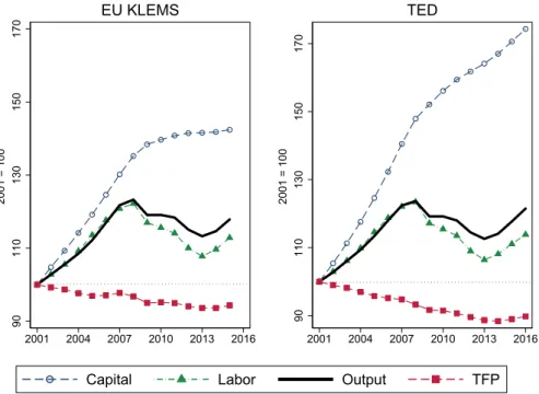
Total Factor Productivity (TFP) is typically defined as the portion of output not explained by the amount of factors used in production. As such, its level is determined by how efficiently the inputs are used in production. Assuming a standard neoclassical production function with labor and capital as the two inputs, TFP could be obtained as the residual (see Appendix B for more details). Figure 1 presents the evolution of Spanish TFP from 2001 to 2016 using both the EU KLEMS and the TED datasets. During the expansion (2001-2007) annual TFP growth was negative: -0.4%
Figure 1: Spanish growth accounting 90 110 130 150 170 2001 = 100 2001 2004 2007 2010 2013 2016 EU KLEMS 90 110 130 150 170 2001 = 100 2001 2004 2007 2010 2013 2016 TED
Capital Labor Output TFP
Notes. Left panel shows the evolution of labor, capital, output and TFP during the period 2001- 2015 according to EU KLEMS. Right panel shows the evolution of labor, capital, output and TFP during the period 2001-2016 according to the Total Economy Database (TED).
according to EU KLEMS data, and -0.9% according to TED data. TFP growth remained subdued during the 2008-2013 recession with annual rates of -0.7% and -1.0% according to EU KLEMS and TED, respectively. Finally, the current recovery (2014-2016) is characterized by the revival of TFP growth. In particular, the annual TFP growth rate based on EU KLEMS is 0.8% in 2014-2015 while this figure is also 0.8% for the 2014-2016 years based on TED data.
Figure 1 also illustrates the impact of the Global Financial Crisis on activity and the accumulation of capital and labor. Both output and labor fell during the crisis while capital growth remained positive, albeit lower. During the 2014-2016 recovery, output and labor growth turned positive and both increased at a similar pace, while the evolution of capital remained similar to that of the 2008-2013 period. Appendix C shows that these patterns are also present when looking at TFP estimates from other sources such as OECD and Banco de Espa˜na. In any event, it is worth highlighting that the increase in the measured capital stock throughout the 2008-2016 period may mask the presence of idle resources in terms of installed equipment (see Banco de Espa˜na Annual Report 2009 Chapter 2 available at https://goo.gl/nJ7xgN), especially at the onset of the crisis.
In order to better understand the drivers of TFP from an aggregate perspective, we re-organize the data in Figure 1 by computing capital-labor (K/L) and output-labor (Y/L) ratios, namely, a measure of capital deepening (K/L) and a measure of labor productivity (Y/L). These two elements
are useful because under a Cobb-Douglas production function with constant returns to scale, log-TFP can be written as the difference between logged labor productivity and logged capital deepening:
logT F P = logY
L −αlog K
L (1)
where α refers to the capital share of the economy. According to EU KLEMS data, α = 1− V AwL remained roughly constant at around 46% in the case of the Spanish economy.5
Moreover, denoting Δ as the first-difference operator, we can write TFP growth (Δ logT F P) as follows:
Δ logT F P = Δ logY
L −αΔ log K
L (2)
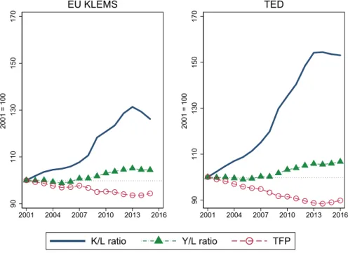
Figure 2 shows that labor productivity remained roughly constant in 2001-2007, increased during the recession, and returned to close-to-zero growth rates over the recovery. This counter-cyclical evolution of labor productivity is a well-known characteristic of the Spanish economy in which em-ployment fluctuations are mostly driven by adjustments in the extensive margin. However, Figure 2 also suggests that the evolution of capital deepening is at the root of the dismal evolution of Spanish TFP until 2013, and the subsequent TFP revival from 2014 to 2016.
During the expansion, depending on the data source the capital-labor ratio grew on average by 1.2-2.3% each year, which combined with flat labor productivity resulted in the negative growth of TFP. In the 2008-2013 recession, labor productivity growth turned positive but capital deepening skyrocketed with annual growth rates of 3.4% and 5.0% according to EU KLEMS and TED, re-spectively (note that this increase does not account for the existence of idle resources in terms of installed equipment). Finally, the fall in the capital-labor ratio during the recent recovery (-2.4% in EU KLEMS data and -0.4% in TED data) coupled with the roughly flat evolution of labor produc-tivity drives the emergence of positive TFP growth rates for the first time since the nineties in the Spanish economy.
2.1
The role of reallocation of resources across industries
The specialization of the Spanish economy in low-TFP sectors such as tourism or construction is typically to blame for the dismal evolution of TFP. In this section, we explore to what extent this hypothesis is at the root of the TFP patterns described above. For that purpose we compute two counterfactual TFPs using industry-level TFP figures from EU KLEMS data combined with two
Figure 2: The evolution of labor productivity and capital deepening 90 110 130 150 170 2001 = 100 2001 2004 2007 2010 2013 2016 EU KLEMS 90 110 130 150 170 2001 = 100 2001 2004 2007 2010 2013 2016 TED
K/L ratio Y/L ratio TFP
Notes. This figure plots the capital-labor ratio (capital deepening), the output-labor ratio (labor productivity), and TFP based on EU KLEMS (left panel) and TED (right panel).
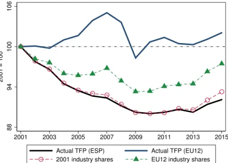
alternative sets of industry-shares.6 On the one hand, we consider the Spanish industry shares for the year 2001, and, on the other hand, we also consider the EU12 contemporaneous industry shares.7 Figure 3 shows the actual evolution of TFP in Spain and the EU12 together with the two coun-terfactual Spanish TFP series. Spanish TFP figures are strikingly different from those of the average EU12 country. During the 2001-2007 expansion years, the fall in Spanish TFP contrasts with the slight increase in EU12 TFP. However, the evolution is somehow similar afterwards: a slight deterio-ration over the crisis (2008-2013) in the EU12 and Spain, followed in both cases by a recovery during the most recent years.
Turning to the counterfactuals, we first use the contemporaneous industry shares in the average EU12 country as weights for each sector. We thus compute the counter-factual TFP that we would have observed in Spain had the Spanish economy featured the industry composition of the average EU12 country (green-triangle dashed line in Figure 3). This counter-factual TFP evolution lies above
6Note that if one aggregates industry TFPs using the observed industry value added shares, the actual Spanish
aggregate TFP would be recovered.
7EU12 includes the following countries: Austria, Belgium, Czech Republic, Denmark, Finland, France, Germany,
Figure 3: The role of industry allocation of resources 88 94 100 106 2001 = 100 2001 2003 2005 2007 2009 2011 2013 2015
Actual TFP (ESP) Actual TFP (EU12)
2001 industry shares EU12 industry shares
Notes. This figure shows the evolution of TFP in Spain (solid black line) and EU12 (solid blue line) together with the evolution of two counter-factual TFPs for Spain: one based on constant industry shares for the year 2001 (red-circle dashed line), and, another one based on contemporaneous industry shares from the EU12 (green-triangle dashed line). The source for all the series is EU-KLEMS.
the actual Spanish TFP, which suggests that part of the low TFP growth in Spain can be attributed to the economic structure of the Spanish economy in which low-productivity industries account for higher shares of value added than other EU12 countries.
Second, we also compute an alternative counter-factual TFP in which we aggregate industry-specific TFP data using the Spanish VA shares in 2001 as weights (constant over time). We also plot this counter-factual TFP in Figure 3 (red-circle dashed line). This counter-factual TFP almost overlaps with the actual TFP evolution throughout the period with only a small improvement after 2013.
All in all, these counterfactual exercises suggest that the reallocation of resource towards low-TFP sectors cannot account for the poor performance of Spanish low-TFP growth. While counterfactual TFPs with constant sector shares are slightly above actual TFP in Figure 3), the aggregate evolution of TFP would have been very similar in all cases, which clearly points to a widespread decline in TFP across sectors during the first years of the crisis, and a generalized recovery over the most recent period. We next turn to the analysis of the role of within-industry —across firms— allocation of resources.
3
Firm-level database
It is well-known that aggregate economic performance strongly depends on firm-level decisions on la-bor and capital markets. Economic analysis has long recognized that behind the observed aggregate behavior of an economy there is widespread heterogeneity in firms’ behavior that must be consid-ered at both theoretical and empirical level. In order to have a better understanding of the TFP performance of Spain over the recent period, we exploit the firm-level dataset taken from Almunia et al. (2018). This administrative dataset contains rich balance-sheet information at the firm level for the non-financial market economy from 2000 to 2016 excluding financial, agricultural and public sectors.8
Our firm-level dataset contains information of around 800,000 firms per year. Compared to the information available from the National Statistics Institute, which contains employment information for the universe of Spanish firms, there are two important aspects to highlight. First, the coverage of our raw sample is remarkably large in terms of both the number of firms (around 80% of the operating firms in Spain) and the level of employment (around 77% of total employment). Second, our sample provides an excellent representation of the firm size distribution in Spain. In particular, small firms (less than 10 employees) account for 83.90% of the total number of firms and 20.47% of the employment in the sample versus 83.07% and 20.23% in the population. At the other extreme, large firms (more than 200 employees) represent less than 0.5% of the total number of firms both in our sample and in the population, while they account for 33.47% of the employment in our sample and 32.13% in the population. An in-depth analysis of this dataset can be found in Almunia et al. (2018).
For each firm, we observe its revenue, value added, total wage bill, employment (number of employees), book value of the capital stock (both physical and intangible), expenses in intermediate goods, and sector of activity at the 4-digit level (according to the NACE rev. 2 classification). Using the information above, we also compute a firm-specic measure of total factor productivity based on Wooldridge (2009) — see Appendix D for details.
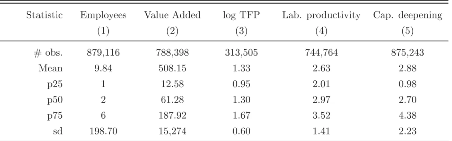
Table 1 provides some basic statistics from our firm-level data for the year 2010. We highlight two main patterns: first, the prevalence of small firms is a key characteristic of the Spanish economy, where the average firm employs around 10 employees but more than 50% of the Spanish companies employ only 2 employees; second, the dispersion in the three measures of productivity is substantial, especially in the case of the capital deepening ratio (K/L). Relative to the firms in the 25th percentile, firms in the 75th percentile present roughly 2.05 log points higher TFPs (i.e. 72 per cent more
8The sample used in this paper is a three-year extension from the previous version constructed by Almunia et al.
Table 1: Firm-level dataset descriptive statistics in 2010
Statistic Employees Value Added log TFP Lab. productivity Cap. deepening
(1) (2) (3) (4) (5) # obs. 879,116 788,398 313,505 744,764 875,243 Mean 9.84 508.15 1.33 2.63 2.88 p25 1 12.58 0.95 2.01 0.98 p50 2 61.28 1.30 2.97 2.70 p75 6 187.92 1.67 3.52 4.38 sd 198.70 15,274 0.60 1.41 2.23
Notes. Employees refers to full-time equivalent employees; value added refers to output in million euros; log TFP refers to the logarithm of total factor productivity; lab. productivity refers to log output-labor ratio; cap. deepening refers to log capital-labor ratio.
productive) according to the figures in Column (3). This figure implies a TFP ratio of e0.72 = 2.05, which indicates that the average firm in the 75th percentile makes around two times as much output with the same measured inputs as the average firm in the 25th percentile. The corresponding 75/25 ratios for labor productivity and capital deepening are 4.53 and 29.96, respectively. Thus, the firm in the 75th percentile of the K/L distribution employs 30 times more capital per unit of labor than the firm in the 25th percentile.9 These differences cannot be explained by differences in the size distribution of firms across industries or years since they remain very similar when we regress the three indicators on a set of size dummies accounting for 2-digit industry and year dummies.
4
From micro to macro: within-industry misallocation
4.1
Measuring misallocation
In this section, we consider two different approaches to estimate the evolution of allocative efficiency across firms over the 2005-2015 period. First, we use the Olley and Pakes (1996) approach, which rests on the static covariance between firms’ market shares and firms’ productivity within each industry. Second, we take into account the role of entry and exit of firms using the dynamic OP covariance developed by Melitz and Polanec (2015). For the sake of completeness, Appendix E reports the
9Note also that there is a sharp drop in the number of observation of log TFP compared to the sample size for
other variables. For instance, there are only 313,505 firms for the variable log TFP while that number is 744,764 and 875,243 for labor productivity and capital deepening, respectively.
results from a fundamentally different measure of misallocation based on the theoretical framework in Hsieh and Klenow (2009).
The allocative efficiency measures based on firm-level data are generally very volatile when looking at their year-on-year evolution so it is advisable to focus on longer time horizons (see e.g. Bartelsman et al. (2013)). Moreover, the role of entry and exit depends crucially on the length of the time period considered as firm churn rates are of course larger for longer time spans. It is thus advisable to analyze subperiods of the same duration in order to ensure comparability. All in all, our baseline analysis is based on two five-year periods, 2005-2010 and 2010-2015, to assess the evolution of misallocation over the first years of the crisis and the subsequent recovery.10
Finally, the allocative efficiency measures (covariances) are computed for each industry at the 4-digit level (according to the NACE rev. 2 classification).11 Then, the industry-specific measures of misallocation are aggregated using industry-specific value added weights to compute aggregate measures of misallocation.
4.1.1 Olley and Pakes 1996
The measure proposed by Olley and Pakes (1996) depends on a decomposition of the aggregate productivity level period-by-period. In particular, aggregate productivity of a given industry at time t, Ψt, can be written as a weighted-average of firm productivities operating in the industry (ψit):12
Ψt =sitψit (3)
where sit refers to the value added share of firm i in year t with isit = 1. Rearranging:
Ψt= ¯ψt+(sit−s¯t)(ψit−ψ¯t) = ¯ψt+cov(sit, ψit) (4) where ¯ψtand ¯strefer to the unweighted averages of productivity and value added shares across firms. Under this decomposition, aggregate productivity can be expressed as the sum of the average firm productivity plus a covariance term capturing the association between market shares and pro-ductivities. Note that the larger this covariance, the larger the allocative efficiency and the aggregate productivity because more productive firms employ a higher share of the resources available in the
10Also, micro-aggregated TFP growth is very similar to TFP growth figures described in Section 2 for these two
subperiods, while the patterns are slightly different when looking at other subperiods due to the high volatilty of the micro-aggregated TFP series.
11Note that aggregate figures reported throughout the paper refer to the whole non-financial market economy
excluding financial, agricultural and public sectors (see Section 3).
12Note that we refer here to productivity in general terms but we will consider three different measures: total factor
4.1.2 Melitz and Polanec 2015
Melitz and Polanec (2015) extend the OP approach to a dynamic setting in which the contribution of the extensive margin (entry and exit) can be accounted for. In a few words, with respect to the static OP decomposition, the dynamic MP decomposition incorporates two additional terms measuring the contribution to aggregate productivity of entrants and exiters. Note that these two contributions are somehow blurred in the case of the static OP approach.
More formally, let sGt = sit represent the aggregate market share of a group G of firms, and define ΨGt = (sit
sGtψit) as the aggregate productivity of this group. Then, aggregate productivity in two consecutive periods, Ψ1 and Ψ2, can be expressed as the sum of the aggregate productivity of the three groups of firms, namely, survivors (S1,S2), entrants (E1,E2), and exiters (X1,X2):
Ψ1 =sS1ΨS1+sX1ΨX1 = ΨS1+sX1(ΨX1−ΨS1) (5) Ψ2 =sS2ΨS2+sE2ΨE2 = ΨS2+sE2(ΨE2−ΨS2) (6) Based on (5) and (6), Melitz and Polanec (2015) decompose the productivity change between periods 1 and 2 (ΔΨ) as follows:
ΔΨ = (ΨS2−ΨS1) +sE2(ΨE2−ΨS2) +sX1(ΨS1−ΨX1) = = Δ ¯ψS+ Δ(covS) +sE2(ΨE2−ΨS2) +sX1(ΨS1−ΨX1)
(7) The first line of equation (7) decomposes the change in aggregate productivity into three com-ponents, namely, the change in productivity for the three groups of firms: survivors (S), entrants (E) and exiters (X). In the second line, the first two terms (Δ ¯ψS + Δ(covS)) refer to the change in the static OP decomposition applied to the group of firms active in both periods (survivors). In particular, the change in the average productivity of the survivors is labeled as the within compo-nent while the change in the covariance is the between compocompo-nent capturing the contribution of the reallocation of resources across firms.
The Melitz and Polanec (2015) decomposition also identifies the contribution of entrants and exiters to the change in aggregate productivity. To be more concrete, the contribution of entry captures the difference in productivity of entrants in period 2 with respect to survivors in that period, i.e., sE2(ΨE2−ΨS2). If entrants are less productive than incumbents, this contribution will be negative. Analogously, the contribution of exit is given by the difference in productivity of exiters industry. Analogously, the change in productivity over time (ΔΨ) is given by the changes in average productivity plus the change in the covariance term, which captures the extent of reallocation of resources across firms.
in period 1 with respect to survivors in that period, i.e., sX1(ΨS1−ΨX1). If exiters present lower productivities than survivors, this contribution will be positive.
4.2
Results
Table 2 presents the results from the OP decomposition applied to our firm-level data in three selected years. Regarding the overall evolution of TFP, labor productivity and capital deepening from our firm level data, we can look at columns (3), (6), and (9). According to the micro data, TFP fell by 8% over the 2005-2010 period while it increased 14% from 2010 to 2015. In contrast, labor productivity growth was rather constant in both subperiods at 7%. Finally, capital deepening shows a much wider variation as suggested by the aggregate figures in Section 2. In particular, it increased around 31% over the 2005-2010 period while it decreased by 54% during the 2010-2015 recovery.13 These figures do not exactly coincide with the aggregate figures in Section 2 but the patterns are qualitatively the same.
Table 2: Olley and Pakes 1996
TFP Lab. productivity Cap. deepening
Covariance Average Total Covariance Average Total Covariance Average Total
(1) (2) (3) (4) (5) (6) (7) (8) (9) 2005 0.65 1.54 2.19 0.28 3.20 3.47 0.27 2.67 2.94 2010 0.61 1.50 2.11 0.34 3.20 3.54 0.30 2.91 3.20 2015 0.75 1.50 2.26 0.33 3.28 3.61 0.08 2.69 2.77 2005-2010 -0.04 -0.04 -0.08 0.07 0.00 0.07 0.03 0.24 0.27 2010-2015 0.14 0.00 0.14 -0.01 0.08 0.07 -0.21 -0.22 -0.43
Notes. TFP refers to the logarithm of total factor productivity; lab. productivity refers to log output-labor ratio; cap. deepening refers to log capital-labor ratio. See section 4.1.1 for details on the Olley and Pakes (1996) approach.
We now turn to the contributions of each term, the change in unweighted averages ( ¯ψt) and the change in the covariance terms measuring allocative efficiency (cov(sit, ψit)). From 2005 to 2010, Table 2 points to a deterioration in TFP due to a mild positive growth of labor productivity coupled with strong growth of capital deepening. The decrease in TFP is explained by both components in the same proportion. Both the average firm-level productivity and the covariance term were reduced by around 4% over the period.
13Note that 27 log points corresponds to a growth rate of 31% (e0.27= 1.31) and 43 log points to 54% (e0.43= 1.54).
Turning to labor productivity, most of the 7% total growth can be attributed to an improvement in allocative efficiency (covariance term) while firm labor productivity remained subdued. This pattern indicates that labor productivity was mainly driven by reallocation of labor from less to
more productive firms between 2005 and 2010. Finally, the 31% increase in capital deepening from 2005 to 2010 is mostly explained by an across-the-board increase in the firm level capital-to-labor ratio while labor reallocation towards more or less capital-intensive firms played a rather limited role (less than 10% of the overall increase).
Between 2010 and 2015, the 14% improvement in TFP can be entirely explained by a better allocation of resources combined with a rather constant average TFP. This implies that high-TFP firms gained market share over the 2010-2015 period. In contrast to the 2005-2010 period, when reallocation was the main driver of labor productivity, the 7% rise during the 2010-2015 period is mainly due to an improvement in the average labor productivity while allocative efficiency remained constant. Finally, the 54% drop in the capital-to-labor ratio can be attributed to a lower average as well as to an improvement in the allocation of resources, i.e., a reallocation of employment towards less capital-intensive firms.
In any case, these findings based on the static OP decomposition do not take into account the role of entry and exit, which might be an important driver of the reallocation process, especially during a crisis. In order to quantify the contribution of this extensive margin, we consider the Melitz and Polanec (2015) methodology that extends the Olley and Pakes (1996) framework to a dynamic setting with entry and exit.
Table 3: Melitz and Polanec 2015
TFP growth Lab. productivity growth Cap. deepening growth
2005-2010 2010-2015 2005-2010 2010-2015 2005-2010 2010-2015 (1) (2) (3) (4) (5) (6) within -0.06 -0.01 0.01 0.09 0.24 -0.21 between -0.02 0.10 0.07 -0.01 0.02 -0.22 entry -0.01 -0.01 -0.01 -0.01 -0.01 -0.01 exit 0.01 0.01 0.02 0.02 0.02 0.02 TOTAL -0.08 0.09 0.09 0.09 0.27 -0.42
Notes. TFP refers to total factor productivity; lab. productivity refers to output-labor ratio; Cap. deepening refers to capital-labor ratio. See section 4.1.2 for details on the Melitz and Polanec (2015) approach.
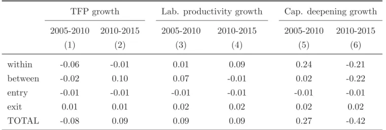
Table 3 presents the results from our preferred approach, the Melitz and Polanec (2015) decom-position. In a few words, the main conclusions from the Olley and Pakes (1996) approach remain valid when also considering the extensive margin in Table 3. This is so because most of the changes can be explained by surviving firms, i.e., movements in the intensive margin.
The extensive margin (entries and exits) plays a very limited role in both sub-periods as well as in all the three variables. In addition to being smaller, the contributions of entry and exit typically cancel out. While new firms are less productive than incumbents leading to a negative entry contribution, exiting firms are also less productive than surviving firms so that the exit contribution is positive. This pattern holds for total factor productivity as well as its two main drivers: labor productivity and capital deepening.
Turning to the intensive margin evolution in Table 3, the picture is essentially the same than in Table 2. The negative growth rate of TFP over 2005-2010 is explained by both a decline in average TFP (within contribution) and a deterioration in allocative efficiency (between contribution). However, the within component driven by a widespread reduction in firms’ TFP seems to be more relevant as it accounts for 6 out of 8 pp. of the overall TFP decline (see column (1) of Table 3).
On the other hand, positive TFP growth between 2010 and 2015 is entirely explained by an improvement in the allocation of resources (between contribution) rather than higher average TFP (within contribution). To be more concrete, column (2) of Table 3 shows that 10 pp. out of the 9 pp. total TFP growth from 2010 to 2015 are due to the between (reallocation) component, while the contribution of the within (average) component is only -1 pp.
Labor productivity growth was mainly driven by a process of employment reallocation from less to more productive firms between 2005 and 2010 but a generalized increase across firms accounts for most of the labor productivity growth from 2010 to 2015. Finally, the 2005-2010 increase in capital deepening can be mostly explained by a generalized surge in the capital-to-labor ratios across firms (within contribution). In contrast, both the within (average) and the between (reallocation) components play a similar role during the 2010-2015 decline in capital deepening.
In terms of misallocation of resources, we conclude from Table 3 that allocative efficiency slightly worsened during 2005-2010 but substantially improved from 2010 to 2015 in terms of TFP. This second result implies that high-TFP firms gained market share between 2010 and 2015 vis-a-vis low-TFP firms. This low-TFP-enhancing process of resource reallocation is mostly driven by labor moving to firms with low capital deepening levels and thus high TFP.
These findings suggest that the main driver of the recent Spanish TFP revival in column (2) of Table 3 is the improvement in the allocation of resources towards high-TFP firms (between contri-bution). Moreover, the reduction in aggregate capital deepening is explained by a reallocation of labor towards firms with low capital-to-labor ratios (see between contribution of -0.22 in column (6) of Table 3). Also, it is worth emphasizing that Spanish firms are reducing the amount of capital per unit of labor required for production as indicated by the within contribution of -0.21 in column (6) of Table 3. In contrast, the fluctuations in the within and between components of labor productivity shown in column (3) are much smaller in magnitude.
5
Concluding Remarks
The dismal performance of total factor productivity (TFP) represents one of the main challenges faced by the Spanish economy since the adhesion to the European Monetary Union in the late nineties. As documented in Garc´ıa-Santana et al. (2016), within-industry misallocation of resources, especially capital, was at the root of the TFP decline from 1995 to 2007. This paper provides an anatomy of the recent evolution of Spanish TFP until 2016.
From an aggregate point of view, TFP growth remained negative during the crisis years but a mild revival of TFP growth appears to characterize the current recovery. The evolution of capital deepening is chiefly responsible of these TFP dynamics, while the role of labor productivity is more muted. In particular, capital deepening accelerated from the onset of the crisis, which slowed down TFP in spite of the improvement in labor productivity. In contrast, capital deepening decelerated significantly since 2013 with the subsequent positive TFP growth for the first time over the last twenty years.14
Turning to the role of the allocation of resources across industries and firms, we conduct sev-eral counterfactual analyses suggesting that the process of reallocation of production factors across industries cannot explain the observed patterns in TFP growth. We thus analyze the role of the within-industry and across firms allocation of resources. Using different measures available from the literature, we conclude that a generalized increase in firms’ capital-to-labor ratios explains most of the TFP decline during the first years of the crisis. In contrast, the TFP revival observed over the last years is mainly driven by the reallocation of labor towards firms with low capital deepening.
A profound analysis of the ultimate causes driving these developments is beyond the scope of this paper. However, the factors behind the deterioration in the allocation of capital until 2007, summarized in Moral-Benito (2018), might shed some light on this question. In particular, a reversion in the (mis?)allocation of credit across firms partially induced by the real estate bubble and the softening of banks lending standards may be a good candidate to explain the current TFP revival. Also, the considerable deleveraging effort made by Spanish firms is chiefly responsible of the TFP-enhancing decline in average capital-to-labor ratios.
14As discussed in the paper, the lack of information on capacity utilization of the installed capital equipment might
play a non-negligible role in these developments because the extent of idle resources is not included in capital stock series based on the perpetual inventory method.
References
[1] Almunia, M., D. L´opez-Rodriguez, and E. Moral-Benito (2018) “Evaluating the Macro-Representativeness of a Firm-Level Database: An Application for the Spanish Economy,” Occa-sional Paper Banco de Espa˜na 1802.
[2] Barro, R. J., and Lee, J. W. (2013) “A new data set of educational attainment in the world, 19502010,”Journal of Development Economics, 104, 184-198.
[3] Bartelsman, E., J. Haltiwanger and S. Scarpetta (2013) “Cross-Country Differences in Produc-tivity,”American Economci Review, 103, 305-334
[4] Byrne, D. and C. Corrado (2016) “ICT prices and ICT services: What do they tell us about productivity and technology,”The Conference Board Economics Program Working Paper Series, EPWP 16-05.
[5] Garc´ıa-Santana, M., E. Moral-Benito, J. Pijoan-Mas, and R. Ramos (2016) “Growing like Spain 1995-2007,” Banco de Espa˜na Working Paper 1609.
[6] Haltiwanger, J., R. Kulick, and C. Syverson (2018) “Misallocation Measures: The Distortion That Ate the Residual,” NBER Working Paper 24199.
[7] Hsieh, C., and P. Klenow (2009) “Misallocation and manufacturing TFP in China and India,”
The Quaterly Journal of Economics, 124, 1403-1448.
[8] Montinari, L., A. Amores and J. Rueda-Cantuche (2016) “Capital indicators for the EU-28 Mem-ber States (1995-2014): Data and methodology of calculations,”Joint Research Centre.
[9] Moral-Benito, E. (2018) “The Microeconomic Origins of the Spanish Boom,” Banco de Espa˜na Occasional Paper 1805.
[10] Olley, S., and A. Pakes (1996) “The Dynamics of Productivity in the Telecommunications Equipment Industry,”Econometrica, 64, 1263-1297.
[11] O’Mahony, M., and M. Timmer (2009) “Output, Input and Productivity Measures at the In-dustry Level: The EU KLEMS Database,” The Economic Journal, 119, 374-403.
[12] Salas, V., L. San Juan and J. Valles (2018) “Corporate Cost and Profit Shares in the Euro Area and the US: The Same Story?” Banco de Espa˜na Working Paper.
[13] Wooldridge, J. (2009) “On estimating firm-level production functions using proxy variables to control for unobservables,”Economics Letters, 104, 112-114.
A
The EUKLEMS and TED databases
Our growth accounting exercises exploit two different data sources, namely, EU KLEMS and TED. Although the patterns arising from these two sources are very similar, it is worth describing the nuances in the methods of collating the data. This section gives more details about the construction of the main variables used in section 2, which are Total Output, Labor Services, Labor Quality and Capital Services from EU KLEMS, and Total Output, Labor Quantity, Labor Quality and Total Capital from TED.
A.1
EU KLEMS
In EU KLEMS, data on Total Output and Capital Services is drawn from Eurostat while data on Labor Services and Labor Quality are sourced from the European Labor Force Survey (EULFS) and the Structure of Earning Survey (SES).
For Total Output, volumes of gross value added (denoted asV A QI in EU KELMS) are denoted in 2010 prices. Also, data on output is consistent with Eurostat at the corresponding industry levels. For constructing labor services series for the period 2008-2015, the main source is the micro-data underlying the European Labor Force Survey (EULFS) provided by the National Institute of Economic and Social Research (NIESR). Years prior 2008 have been extrapolated using the trend in labor services from former versions of EU KLEMS.
Turning to the estimation of Labor Quality, it combines different sources of information. First, information on the employment structure of the workforce, such as age, gender and educational attainment level is obtained from EULFS. In particular, two gender categories (male, female), three age categories (15-29, 30-49, 50 and above) and three educational qualification levels (high, medium and low) are considered. Second, data on wages are drawn from the Structure of Earning Survey (SES). Since the micro data underlying SES is not yet available for the most recent survey, EU KLEMS uses the available SES tabulation from Eurostat to obtain wage figures for 2010 and 2014.
The Capital Services variable is estimated using different depreciation rates depending on the type of asset. Depreciation rates for computing equipment, communications equipment, software and databases, transport equipment, other machinery, total non-residential investment and other assets are taken form previous EU KLEMS releases, the depreciation rate for research and development is taken from the SPINTAN project, and depreciation rates for other asset types stems from Montinari et al. (2016).
A.2
TED
In the TED database, Total Output is sourced from Eurostat, Labor Quantity is drawn from the OECD, and Labor Quality is taken from the EU KLEMS database. Total Capital is constructed combining all the three databases, EU KLEMS, OECD and Eurostat.
For Labor Quantity, TED gives a clear definition. The employment figures cover all persons engaged in some activity that falls within the production boundary of the system of national accounts. In line with the GDP, it includes all workers employed domestically but excludes any nationals working abroad. The measure used in TED is actual hours worked, so it includes paid overtime and excludes paid hours that are not worked due to sickness, vacation and holidays etc.
For Labor Quality, TED used a similar method in computing the indicator as EU KLEMS. This indicator is constructed using data on employment and compensation by educational attainment where the data is collected from various source, including Eurostat, World Input Output Database (W IOD) and various country-specific KLEMS databases. The growth rate of labor quality is cal-culated as the the difference between labor input growth rates, measured as a labor composition weighted growth rate of individual skill categories of workers, and labor quantity growth rates, mea-sured as the growth rate of aggregate hours or employment. The underlying assumption used in the regression to estimate labor compensation by educational attainment is that the returns to educa-tion are broadly similar across countries in a given region for a given educaeduca-tional category. Lastly, Data on average years of schooling by educational attainment (primary, secondary and tertiary) from Barro and Lee (2013) are combined with the available data on the structure of labor compensation by educational attainment.
Lastly, growth in total capital services refers to change in the flow of productive services by capital assets. The underlying capital stock series for six different asset types are calculated from National Accounts investment data using the perpetual inventory method (PIM). The aggregation of the growth in capital services over the different asset types is calculated using the user cost approach. To compute the deflator for ICT investment, alternative price measures developed by Byrne and Corrado (2016) are used as recent evidence suggests that the official deflators underestimate the true price decline (only for the aggregate economy). Investment price deflators for ICT assets are obtained from National Accounts whenever available. For most advanced economies, these deflators are quality adjusted hedonic prices, which are assumed to be taking into account the rapid changes in the quality of ICT goods, and hence the price decline. However, it is argued that the official hedonic prices for ICT goods still understate the rapid declines in prices (Byrne and Corrado, 2016). To take the impact of this rapid price declines into account, an alternative set of investment, capital stock, and thus the entire growth accounting variables are constructed in the TED using this alternative ICT price deflators to deflate ICT investment goods (hardware, communication equipment and software).
B
Methodological details about aggregate TFP estimates
B.1
EU KLEMS
The methodology used in EU KLEMS is based on a production function approach where industry gross output is a function of capital, labor, intermediate inputs and technology, which is indexed by time, T. Each industry, indexed by j, can produce a set of products and purchases a number of distinct intermediate inputs, capital and labor to produce its output. The production function is given by:
Yj =fj(Kj, Lj, Xj, T) (8)
where Y is output, K is an index of capital service flows, L is an index of labor service flows and X is an index of intermediate inputs, either purchased from domestic industries or imported. Under the assumptions of competitive factor markets, full input utilization and constant returns to scale, the growth of output can be expressed as the cost-share weighted growth of inputs and Hicks-neutral technical change A. Using the translog functional form:
Δ ln(Yjt) = ¯vjtXΔ ln(Xjt) + ¯vKjtΔ ln(Kjt) + ¯vjtLΔ ln(Ljt) + ln(AYjt) (9) where ¯vi denotes the two-period average share of input i in nominal output defined as follows:
vX jt = PX jt ∗Xjt PY jt ∗Yjt ;vLjt = P L jt∗Ljt PY jt ∗Yjt ;vKjt = P K jt ∗Kjt PY jt ∗Yjt (10) and ¯vX + ¯vL+ ¯vK = 1.
Each element on the right-hand side of the above equations indicates the proportion of output growth accounted for by growth in intermediate inputs, capital services, labor services and technical change as measured by total factor productivity (TFP), respectively. It is common to define aggregate input, say labor, as a T¨ornqvist quantity index of individual labor types as follows:
Δ ln(Ljt) = l ( ¯wLl,jtΔ ln(Ll,jt)) (11) Δ ln(Kjt) = k ( ¯wKk,jtΔ ln(Kk,jt)) (12) Δ ln(Xjt) = x ( ¯wx,jtX Δ ln(Xx,jt)) (13)
where Δ ln(Ljt) indicates the growth of hours worked by labor type l and weights are given by the period average shares of each type in the value of labor compensation, and similarly for K and X. As we assume that marginal revenues are equal to marginal costs, the weighting procedure ensures that inputs which have a higher price also have a larger influence in the input index. So for example a doubling of hours worked by a high-skilled worker gets a bigger weight than a doubling of hours worked by a low-skilled worker.
EU KLEMS also separate total intermediate inputs into three groups: energy, materials and services (E, M, S). To analyze the separate impact of ICT and non-ICT (N) capital, capital input growth can be divided into these two groups of assets. In terms of labor inputs, it is useful to split the volume growth of labor input into the growth of hours worked (H) and the changes in labor composition (LC) in terms of labor characteristics such as educational attainment, age or gender.
As such, the EU KLEMS database provides a full decomposition of growth in gross output into eight elements as follows:
Δ ln(Yjt) = ¯vjtXw¯jtEΔ ln(XjtE) + ¯vjtXw¯MjtΔ ln(XjtM) + ¯vjtXw¯SjtΔ ln(XjtS) (14) + ¯vjtKw¯jtICTΔ ln(KjtICT) + ¯vKjtw¯jtNΔ ln(KjtN) (15) + ¯vjtLΔ ln(LCjt) + ¯vjtLΔ ln(Hjt) + Δ ln(AYjt) (16) The contribution of each intermediate and capital input is given by the product of its share in total costs and its growth rate. The contribution of labor input is split into hours worked and changes in the composition of hours worked, and any remaining output growth is picked up by the total factor productivity termA (this term is also known as multi-factor productivity).
B.2
TED
Similarly to EU KLEMS, TFP estimates from TED consider the standard growth accounting frame-work in which GDP growth can be decomposed into contributions from factor inputs, capital (K), and labor (L) and total factor productivity (T F P) under the assumption of Cobb-Douglas production function:
Δ ln(GDP) = ¯vKΔ ln(K) + ¯vLΔ ln(L) + Δ ln(T F P) (17) where Δ ln(X) indicates the growth rate (measured in log changes) of any given variables X (GDP, K,LandT F P). ¯vK and ¯vLdenote respectively the share of capital compensation and labor compen-sation in nominal GDP, both averaged over the current and previous year. Under constant returns to scale, i.e. ¯vK + ¯vL = 1, the capital compensation share can be obtained by subtracting labor compensation from nominal value added.
The contribution of labor input to GDP growth in TED is split into the contribution of employ-ment quantity (H) and labor composition or quality (LQ), and the contribution of capital services is split into ICT capital services (Kit) and non-ICT capital services (Knit):
Δ ln(GDP) = ¯sK,itΔ ln(Kit) + ¯sK,nitΔ ln(Knit) + ¯sLΔ ln(H) + ¯sLΔ ln(LQ) + Δ ln(T F P) (18) where ¯sK,it and ¯sK,nit are respectively the shares of ICT capital and non-ICT capital income in nominal GDP.
To summarize, this equation decomposes the growth in GDP into contribution from labor and capital inputs (weighted by their respective shares in nominal GDP) and a residual labeled TFP growth. Under neoclassical assumptions, this refers to technological change or the overall efficiency of the economy.
B.3
OECD
similarly to EU KLEMS, OECD considers an aggregate production function featuring Hicks neutral technical change, as it is represented as an outward shift of the production function that affects all factors of production proportionately:
Q=Af(L, K) (19)
Differentiating this expression with respect to time and using a logarithmic rate of change, multi-factor productivity growth (the rate of change of the variable A, also known as total factor produc-tivity growth) is measured as the rate of change of volume output (Q) minus the weighted rates of change of inputs (X). In this simple terms, growth in multifactor productivity (MFP) can be described as the change in output that cannot be explained by changes in the quantity of capital and labor inputs used to generate output. MFP (or TFP) growth is then measured as follows:
ln( Xt Xt−1) = ln( Qt Qt−1)−ln( Xt Xt−1) (20)
where Q is output measured as GDP at market prices and constant prices;X refers to total inputs used and the rate of change of these inputs is calculated as a weighted average of the rate of change of labor and capital inputs, with the respective cost shares as weights. Aggregation of these inputs is done using the Trnqvist index:
ln( Xt Xt−1 ) = 1 2(s t L+stL−1) ln(LLt t−1 ) + 1 2(s t K+stK−1) ln(KKt t−1 ) (21)
B.4
Banco de Espa˜
na (BdE)
Banco de Espa˜na TFP figures are estimated using data taken from AMECO, the annual macro-economic database of the European Commission’s Directorate General for Economic and Financial Affairs. Similarly to the previous sources, TFP growth approximates the difference between the growth in GDP and the growth of primary inputs (capital and labor) weighted by their shares in total income. To be more concrete, Banco de Espa˜na adjust the capital stock series based on Nu˜nez and Perez (2002).15
C
Spanish TFP figures from alternative sources
Figure C.1: The evolution of Spanish TFP 2000-2016
80 90 100 110 2001 = 100 2001 2003 2005 2007 2009 2011 2013 2015
BdE EUKLEMS TED OECD
Notes. This figure shows the evolution of Spanish TFP (2001 = 100) using TFP estimates from different sources: Banco de Espa˜na (BdE), EU KLEMS, TED and OECD.
15See “Estimacion de los stocks de capital productivo y residencial para Espaa y la UE”, Banco de Espa˜na, Boletin
Economico, October 2002.
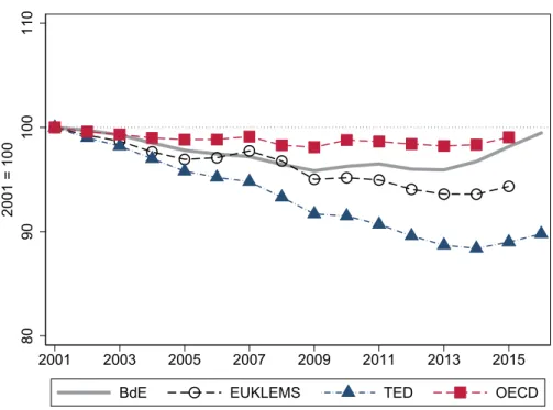
Figure C.1 plots the different paths of Spanish TFP emerging from the different data sources described in Section B. TFP from the TED database (blue triangle dashed line) provides the most pessimistic picture, with an average decline of 0.7% per year between 2001 and 2016. TFP calculated
from the EU KLEMS dataset (black circle dashed line) shows a smaller decline compared to TED, but a larger drop compared to Banco de Espa˜na TFP series (grey solid line) and OECD TFP series (red square dashed line). These differences are more marked after 2013, when estimates from Banco de Espa˜na and OECD imply a full recovery of TFP to the level in 2001, whereas EU KLEMS and TED still suggest that TFP is only 94.3% and 89.8% of the level in 2001, respectively. In any event, it is reassuring that all the four TFP series point to the same general patterns uncovered in this paper: the growth of Spanish TFP was negative in the early years of the crisis until 2013, but turned positive during the current recovery period.
D
Methodological details about firm-level TFP estimates
The object of interest is the TFP of firm i in year t, labeled as ait in the following equation derived from a firm-specific Cobb-Douglas production function:
yit =αLlit+αKkit+αMmit+ait (22)
whereyrefers to logged output, andl,k, andmare logged labour, capital, and materials, respectively. The estimation of equation (22) is performed on a 2-digit industry level. However, in order to obtain consistent estimates with sufficient degrees of freedom, a cutoff of a minimum of 25 observa-tions per sector and year is introduced. Sectors that do not meet the minimum cutoff are flagged and their TFP estimates are replaced by an estimated value obtained on the corresponding macro-sector level. A full set of year dummies is included to control for sector-specific trends.
To estimate the parameters in the production function, we assume that ait is the sum of two firm-specific and unobserved components, namely, a component which is known to the firm (ωit), and a component unknown to the firm and with no impact on firm’s decisions (vit). The endogeneity problem that renders OLS estimates biased when estimating equation (22) arises from the correlation of ωit with the input choices. One of the solutions provided for solving this problem is introduced by Olley-Pakes (1996) who proposed a structural approach to the problem, by using observed input choices to instrument for unobserved productivity. In particular, their approach relied upon the assumption that investment, iit, installed in period t only becomes productive at t+ 1, so that iit= i(ωit;kit) can be inverted to yield ωit = ω(iit;kit) under the assumption of increasing monotonicity of iit inωit.
Finally, Wooldridge (2009) introduces an appealing GMM approach that implements this identi-fication strategy reducing the computational burden as well as producing more efficient estimates.
E
Dispersion measures of misallocation
In this section, we analyze the evolution of within-industry misallocation from a different perspective that is widely-used in the literature, the so-called Hsieh and Klenow variances. While the Olley and Pakes (1996) and Melitz and Polanec (2015) measures are model-free to the extent that they are based on simple covariances from the data, the Hsieh and Klenow (2009) measure depends on a theoretical framework in which marginal revenue productivities of capital and labor should equalize across firms and within-industries under the assumption that the production technology is common to all firms in a given industry. An increase in within-industry variances of marginal productivities indicates that allocative efficiency is worsening.
The key intution of the Hsieh and Klenow (2009) approach is that in a frictionless economy one should observe no dispersion in firm-level revenue productivities (for both capital and labor) within each industry because higher productivity firms should expand, attracting more capital and workers, which in turn would diminish their revenue productivity (either because of decreasing returns to scale or because of downward-sloping demand curves). Hence, dispersion of revenue productivities across firms is a symptom of a poor allocation of resources across firms.16 In their framework, an efficient / frictionless allocation of resources implies the maximum possible TFP and equal marginal productivities (of both capital and labor) for all firms within each industry. Hence, any heterogeneity in marginal revenue productivities across firms operating in the same 4-digit industry is interpreted as a measure of misallocation.
Based on the Hsieh and Klenow (2009) framework, we compute the marginal revenue product of labor and capital for each firm as well as the revenue TFP. Then, we compute the industry-specific variances of all the three elements and its evolution over time to assess the extent of within-industry misallocation according to this metric.
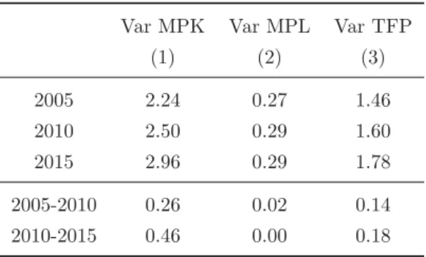
Table E.1 presents the evolution of these variances in our firm level data. In contrast to the findings based on the Olley and Pakes (1996) and Melitz and Polanec (2015) covariances, allocative efficiency deteriorated in both subperiods 2005-2010 and 2010-2015 according to column (3). How-ever, increases in the TFP variance are mostly driven by the misallocation of capital in column (1), which is in line with our finding based on OP and MP decompositions that capital deepening seems to be more important than labor productivity to explain TFP developments over time.
16Hsieh and Klenow (2009) take the US economy as a benchmark and show that lower TFP in China and India can
In any event, it is worth highlighting that there is an open debate in the literature about the comparability of the different misallocation measures. The reader interested in more details is referred to Haltiwanger et al. (2018) and the references cited therein.
Table E.1: Hsieh and Klenow 2009
Var MPK Var MPL Var TFP
(1) (2) (3) 2005 2.24 0.27 1.46 2010 2.50 0.29 1.60 2015 2.96 0.29 1.78 2005-2010 0.26 0.02 0.14 2010-2015 0.46 0.00 0.18
Notes. MPL and MPK refer to marginal rev-enue products of labor and capital, respectively.
BANCO DE ESPAÑA PUBLICATIONS
OCCASIONAL PAPERS
1101 LUIS ORGAZ, LUIS MOLINA and CARMEN CARRASCO: El creciente peso de las economías emergentes en la economía y gobernanza mundiales. Los países BRIC.
1102 KLAUS SCHMIDT-HEBBEL: Central banking in Latin America: changes, achievements, challenges. (There is a Spanish version of this edition with the same number).
1103 OLYMPIA BOVER: The Spanish Survey of Household Finances (EFF): description and methods of the 2008 wave. 1104 PABLO HERNÁNDEZ DE COS, MARIO IZQUIERDO and ALBERTO URTASUN: An estimate of the potential growth of
the Spanish economy. (There is a Spanish version of this edition with the same number).
1105 ENRIQUE ALBEROLA, CARLOS TRUCHARTE and JUAN LUIS VEGA: Central banks and macroprudential policy. Some refl ections from the Spanish experience.
1106 SAMUEL HURTADO, ELENA FERNÁNDEZ, EVA ORTEGA and ALBERTO URTASUN: Nueva actualización del modelo trimestral del Banco de España.
1107 PABLO HERNÁNDEZ DE COS and ENRIQUE MORAL-BENITO: Health care expenditure in the OECD countries: effi ciency and regulation. (There is a Spanish version of this edition with the same number).
1201 ELOÍSA ORTEGA and JUAN PEÑALOSA: The Spanish economic crisis: key factors and growth challenges in the euro area. (There is a Spanish version of this edition with the same number).
1202 MARÍA J. NIETO: What role, if any, can market discipline play in supporting macroprudential policy?
1203 CONCHA ARTOLA and ENRIQUE GALÁN: Tracking the future on the web: construction of leading indicators using internet searches. (There is a Spanish version of this edition with the same number).
1204 JOSÉ LUIS MALO DE MOLINA: Luis Ángel Rojo en el Banco de España.
1205 PABLO HERNÁNDEZ DE COS and CARLOS THOMAS: El impacto de la consolidación fi scal sobre el crecimiento económico. Una ilustración para la economía española a partir de un modelo de equilibrio general.
1206 GALO NUÑO, CRISTINA PULIDO and RUBÉN SEGURA-CAYUELA: Long-run growth and demographic prospects in advanced economies.
1207 IGNACIO HERNANDO, JIMENA LLOPIS and JAVIER VALLÉS: Los retos para la política económica en un entorno de tipos de interés próximos a cero.
1208 JUAN CARLOS BERGANZA: Fiscal rules in Latin America: a survey.
1209 ÁNGEL ESTRADA and EVA VALDEOLIVAS: The fall of the labour income share in advanced economies. 1301 ETTORE DORRUCCI, GABOR PULA and DANIEL SANTABÁRBARA: China’s economic growth and rebalancing. 1302 DANIEL GARROTE, JIMENA LLOPIS and JAVIER VALLÉS: Los canales del desapalancamiento del sector privado: una
comparación internacional.
1303 PABLO HERNÁNDEZ DE COS and JUAN F. JIMENO: Fiscal policy and external imbalances in a debt crisis: the Spanish case.
1304 ELOÍSA ORTEGA and JUAN PEÑALOSA: Algunas refl exiones sobre la economía española tras cinco años de crisis. 1401 JOSÉ MARÍA SERENA and EVA VALDEOLIVAS: Integración fi nanciera y modelos de fi nanciación de los bancos
globales.
1402 ANTONIO MONTESINOS, JAVIER J. PÉREZ and ROBERTO RAMOS: El empleo de las Administraciones Públicas en España: caracterización y evolución durante la crisis.
1403 SAMUEL HURTADO, PABLO MANZANO, EVA ORTEGA and ALBERTO URTASUN: Update and re-estimation of the Quarterly Model of Banco de España (MTBE).
1404 JUAN CARLOS BERGANZA, IGNACIO HERNANDO and JAVIER VALLÉS: Los desafíos para la política monetaria en las economías avanzadas tras la Gran Recesión.
1405 FERNANDO LÓPEZ VICENTE and JOSÉ MARÍA SERENA GARRALDA: Macroeconomic policy in Brazil: infl ation targeting, public debt structure and credit policies.
1406 PABLO HERNÁNDEZ DE COS and DAVID LÓPEZ RODRÍGUEZ: Tax structure and revenue-raising capacity in Spain: A comparative analysis with the UE. (There is a Spanish version of this edition with the same number).
1407 OLYMPIA BOVER, ENRIQUE CORONADO and PILAR VELILLA: The Spanish survey of household fi nances (EFF): description and methods of the 2011 wave.
1501 MAR DELGADO TÉLLEZ, PABLO HERNÁNDEZ DE COS, SAMUEL HURTADO and JAVIER J. PÉREZ: Extraordinary mechanisms for payment of General Government suppliers in Spain. (There is a Spanish version of this edition with the same number).