Time-consistent consumption taxation

Economics Working Paper Series

2014/022

Time-Consistent Consumption Taxation

Sarolta Laczó and Raffaele Rossi

The Department of Economics Lancaster University Management School

Lancaster LA1 4YX UK

© Authors

All rights reserved. Short sections of text, not to exceed two paragraphs, may be quoted without explicit permission,

provided that full acknowledgement is given.

Time-Consistent Consumption Taxation

∗

Sarolta Lacz´

o

Raffaele Rossi

October 2014

Abstract

We characterise optimal fiscal policies when the government has access to consumption taxa-tion but cannot credibly commit to future policies, in a calibrated Real Business Cycle model of the United States economy. Contrary to the case where only labour and capital income are taxed, the optimal time-consistent policies are remarkably similar to their Ramsey coun-terparts, as long as the capital income tax causes some distortion within the period. The welfare gains from commitment are negligible, while they are substantial without consump-tion taxaconsump-tion. Further, the welfare gains from taxing consumpconsump-tion are much higher without commitment. These results suggest that the policy-maker’s ability to commit is of secondary importance if consumption is taxed optimally.

JEL classification: E62, H21.

Keywords: fiscal policy, Markov-perfect policies, consumption taxation, variable capital utilisation, endogenous government spending.

∗_{This paper has greatly benefited from discussions with Charles Brendon, Davide Debortoli, Andrea Lanteri,} Campbell Leith, Yang K. Lu, Albert Marcet, Ricardo Nunes, Evi Pappa, Vito Polito, and Maurizio Zanardi. We also thank seminar participants at CREI/UPF, IAE/UAB, Bank of England, and Lancaster University, and participants of the Max Weber June Conference in Florence, the Barcelona GSE Summer Forum ‘Macro and Micro Perspectives on Taxation,’ CEF in Oslo, PET in Seattle, EEA in Toulouse, and MMF in Durham for useful comments and suggestions. We received funding from the Spanish Ministry of Science and Innovation under grant ECO2008-04785 and the European Community’s Seventh Framework Programme (FP7/2007-2013) under grant agreement no. 612796. Lacz´o also acknowledges funding from the JAE-Doc programme co-financed by the European Social Fund. Rossi thanks the Institut d’An`alisi Econ`omica (IAE-CSIC) for hospitality during May and June 2014. All errors are our own.

†_{Institut d’An`alisi Econ`omica (IAE-CSIC) and Barcelona GSE, Campus UAB, 08193 Bellaterra, Barcelona,} Spain. Email: [email protected].

‡_{Department of Economics, Lancaster University Management School, LA1 4XY, Lancaster, United Kingdom.} Email: [email protected].

1

Introduction

Most of the literature on optimal fiscal policy rules out consumption taxation, a policy instrument which is used in most industrialised economies. For example, in 2013 the value-added tax on standard items ranged from 15 to 27 percent in European Union countries. Papers which consider consumption taxation include Coleman (2000), who finds, under the assumption that the fiscal authority can fully commit to future policies, that replacing income taxes with consumption taxes would lead to a large welfare gain in the United States. Correia

(2010) extends this result to a heterogeneous agents framework. Two recent contributions highlight the role of consumption taxation as a tool to relax a constraint of the monetary authority on the nominal interest rate, either as a result of the zero lower bound (Correia, Farhi, Nicolini, and Teles, 2013) or in a monetary union (Farhi, Gopinath, and Itskhoki,

2014).

This paper finds a new benefit of consumption taxation: discretionary policies and the resulting allocations are almost identical to those under Ramsey policy. This holds for the steady state, for policy dynamics in a deterministic framework, and for the cyclical properties of tax rates and allocations in a stochastic environment. A necessary condition for these findings is that capital income taxation causes some distortion within the period. This means that the policy-maker’s ability to commit is of secondary importance as long as consumption can be taxed. In other words, the negative effects of policy-makers’ lack of credibility, due to political business cycles, political disagreement, default on past promises, etc., can be overcome by taxing consumption optimally.

The novelty of our paper lies in analysing time-consistent fiscal policy when the policy-maker has access to consumption taxation, in addition to labour and capital income taxation. The existing literature on Markov-perfect policies has not considered consumption taxation, to our knowledge. We are able to quantify the welfare gains from taxing consumption and from commitment, as well as the potential welfare gains from implementing optimal time-consistent policies compared to the existing tax system in the United States.

The model economy we consider is a standard Real Business Cycle (RBC) model with endogenous labour supply and variable capital utilisation (Greenwood, Hercowitz, and Huff-man, 1988, among others). The government spends on public goods which households value, has access to three types of taxes, capital and labour income taxes and consumption taxes, but no lump-sum taxes, and has to balance its budget. We exclude public debt dynamics for two main reasons. First, we wish to compare our findings with previous studies on time-consistent fiscal policies with capital accumulation, which also impose a balanced-budget requirement (Klein, Krusell, and R´ıos-Rull,2008;Martin, 2010;Debortoli and Nunes,2010).

Second, in an RBC model with variable capital utilisation, Ramsey policies can be made time consistent through public debt restructuring (Zhu, 1995). Dom´ınguez (2007) establishes a similar result when there are delays in tax policy implementation. Excluding public debt in models with capital accumulation increases the time-inconsistency of Ramsey taxation, and allows us to better isolate the role of consumption taxation.

Our paper is at the intersection of two strands of the optimal taxation literature: (i) Ramsey policies with consumption taxation, such as Coleman (2000), who quantifies the welfare gains from taxing consumption; and (ii) time-consistent policies without consumption taxation. The latter strand of the literature finds that lack of commitment alters greatly the characteristics of optimal policies and the resulting allocations. In a framework similar to ours but with capital fully utilised, Klein, Krusell, and R´ıos-Rull (2008) find that when the only tax base available to the government is capital income, which in their Markov-perfect equilibrium is an inelastic source of fiscal revenues, the policy-maker sets the tax rate below the confiscatory level. Martin (2010) studies a Markov-perfect equilibrium in which the fiscal authority can simultaneously tax labour and capital income. He finds that the optimal policy calls for taxing capital and subsidising labour when capital is fully utilised. With endogenous capital utilisation, as in the present paper, he finds that optimal time-consistent taxation involves almost equal tax rates on capital and labour income, which are close to the existing tax rates in the United States. Debortoli and Nunes (2010) also establish the same quantitative result.

Our results can be summarised as follows. If the policy-maker has access to all three types of taxes and the tax rates are unrestricted, the first-best allocation can be implemented at the steady state under full commitment. Given that the Ramsey policy achieves the first best, it is also time-consistent. In other words, the solutions under Ramsey and Markov-perfect policy-making coincide at the steady state. However, the tax policies include a large labour subsidy.

Then, we study the case where the government is prohibited from subsidising labour income, as in Coleman (2000) and Correia (2010), because large labour subsidies are not observed in real economies and would likely lead to misreporting of hours. In this case, the Ramsey policy-maker taxes consumption at 22.3 percent at the steady state in our baseline calibration, and sets labour and capital income taxes to zero. The time-consistent policy-maker finances government spending mainly from taxing consumption as well, taxing it at 22.1 percent in our baseline calibration, and sets the capital income tax to 0.4 percent and the labour income tax to zero. In order to compare our results with the literature, e.g.Martin

(2010) andDebortoli and Nunes(2010), we also analyse a scenario in which the policy-maker can only tax income deriving from labour and capital. In this case, the time-consistent

policy-maker sets the labour income tax to 6.5 percent and the capital income tax to 19.8 percent at the steady state.

The intuition behind these results is the following. With only labour and capital income taxation, the Ramsey planner initially taxes capital at a high rate. Then the capital tax rate gradually approaches zero, while the labour income tax rate increases over time. The downward trend in the capital income tax induces households to continuously postpone their consumption, while a labour tax hike reduces labour supply contemporaneously, but raises it in any previous period. The time-consistent policy-maker does not internalise the effects of taxes on private sector decisions in earlier periods. This leads to dramatic differences of policies and allocations between Ramsey and Markov-perfect governments.

On the contrary, with access to consumption taxation, a downward trend in the capi-tal tax would require an upward trend in the consumption tax to satisfy the government’s budget constraint. This would counteract the saving incentive and lead to inefficiently low capital accumulation. As a result, the capital income tax rate is low from the start, and the consumption tax rate hardly varies over time or with the level of capital. Thus the time-inconsistency features of policies under commitment are negligible when consumption is taxed optimally. This is the key economic mechanism that drives the close similarities between Ramsey and Markov-perfect policy equilibria. Note also that while both taxes cause an intratemporal distortion, the capital income tax causes an intertemporal distortion as well in the long run, since it distorts the Euler equation, while the consumption tax does not. Therefore, taxing consumption turns out to be the less distortive way to raise fiscal revenue. In terms of welfare-equivalent consumption, the welfare gains from taxing consumption are 2.77 (1.21) percent in the case of a Markov (Ramsey) policy-maker. This means that taxing consumption generates much larger welfare gains under discretion than under commitment. The gains from commitment are negligible with consumption taxation (0.0003 percent), while they are substantial (2.01 percent) without.

We also compute the welfare gain from adopting the time-consistent tax system with consumption taxation proposed here over the existing one in the United States. The welfare increase is equivalent to permanently increasing consumption by 7.744 percent. Without access to consumption taxation, the welfare gain is 4.92 percent. In the case of a Ramsey policy-maker, the welfare gains are 7.745 and 7.06 percent with and without access to con-sumption taxation, respectively. Remarkably, we find higher levels of welfare under discretion when the policy-maker has access to consumption taxation than under commitment when the government can tax only labour and capital income.

Finally, we analyse policies over the business cycle when the economy is hit by aggre-gate productivity shocks. We find that with access to consumption taxation, the cyclical

properties of tax rates and allocations under a Ramsey and a time-consistent policy-maker are remarkably similar. Further, private consumption, hours, public goods, and output all vary less over the business cycle with consumption taxation than without. Hence, the policy-maker can better stabilise the economy taxing consumption, which yields additional welfare benefits.

The rest of this paper is structured as follows. Section2details the economic environment. Section3first defines our policy equilibria of interest, (i) the Ramsey/full-commitment equi-librium and (ii) the Markov/time-consistent equiequi-librium. Afterwards, it characterises these equilibria and presents some analytical results. Section 4 contains our baseline quantitative results, both in a deterministic and in a stochastic environment, as well as robustness checks. Section 5concludes.

2

The model

We consider a discrete-time RBC model with a representative household, a representative and perfectly-competitive firm, and a benevolent policy-maker. The household decides on consumption and leisure and chooses a capital utilisation rate as well (see Greenwood, Her-cowitz, and Huffman, 1988, Greenwood, Hercowitz, and Krusell, 2000, and many others). The firm maximises profits and uses capital services and labour as production inputs.

The policy-maker spends on public goods which yield utility to the household, and raises revenue via linear taxes on labour and capital income as well as on consumption. Lump-sum taxes are not available. The government balances its budget in each period.1 _{Next we}

describe the economic environment in detail.

The representative household takes prices and policies as given and seeks to maximise

E0 " _∞ X t=0 βtu(ct, `t, gt) # , (1)

where _E0 represents the rational-expectations operator at time 0, β ∈ (0,1) is the discount

factor, ct is private consumption,`t represents leisure, and gt is public consumption; subject to the time constraint

ht+`t= 1, (2)

where ht represents hours worked, and the budget constraint (1 +τ_tc)ct+kt+1 = 1−τtk

rtvtkt+ 1−τth

wtht+ (1−δ(vt))kt, ∀t, (3)

1_{As discussed above, this is a common approach in the literature that studies Markov-perfect policies in}

models with capital accumulation (Klein and R´ıos-Rull,2003;Ortigueira,2006;Klein, Krusell, and R´ıos-Rull,

2008;Azzimonti, Sarte, and Soares,2009;Martin,2010;Debortoli and Nunes,2010). Furthermore, we want to rule out the possibility of making the Ramsey policy time consistent through debt restructuring, seeZhu

wherektis the level of the capital stock at the beginning of the period,vt ∈(0,1] is the capital utilisation rate, δ(vt) represents the depreciation rate as a function of capital utilisation,

τc

t, τth, and τtk denote the consumption, the labour income, and the capital income tax rate, respectively. Finally, the variables rt and wt are the interest rate and the wage rate, respectively, and represent the remuneration of production factors, namely, capital services and labour. The utility function u() is assumed to be twice continuously differentiable in all three of its arguments with partial derivatives uc,t >0, ucc,t <0, u`,t >0, u``,t <0, ug,t>0,

ugg,t <0, where ux,t and uxx,t denote, respectively, the first and the second derivative of the utility function with respect to the variable x at time t.

Note that it is crucial that at least some true economic depreciation is not tax deductible, else the current government would view the current capital tax as non-distortionary, and the policy problem of the optimal time-consistent tax mix would reduce to a trivial exercise (see

Martin(2010) for a discussion). In reality the depreciation allowance does not depend on the actual depreciation rate or the capital utilisation rate, instead it depends on the accounting value of capital and a fixed depreciation rate determined by law. This means that capital income taxation indeed distorts the capital utilisation margin and therefore is distortionary within the period.2,3

Combining the first-order conditions with respect to consumption and leisure at time t

gives u`,t uc,t = 1−τ h t 1 +τc t wt. (4)

Defining the price at time t as

qt= t Y s=0 1−δ(v0) + 1−τ0k v0r0 1−δ(vs) + (1−τsk)vsrs (5)

and taking first-order conditions with respect to consumptions at different points in time, the Euler equation between 0 and any t can be expressed as

uc,0 1 +τc 0 =βt_E0 uc,t 1 +τc t 1 qt , (6)

2_{We do not introduce the accounting value of capital into our model, as inMertens and Ravn(2011) for}

example, because not only we would have an additional endogenous state variable, but also the (forward-looking) Euler equation would include all future capital utilisation and capital income tax rates on the right hand side. Hence, recasting the problem into a recursive form and in turn solving it appear challenging.

3_{Instead of endogenous capital utilization, Klein and R´ıos-Rull (2003) assume that the capital income}

tax is chosen one or more periods in advance. In this way the current government internalises the distortive effects ofτk _{on future allocations. This approach, however, raises the question of why the capital income tax}

would be set before other taxes. Note, however, that also in this case the Ramsey policy can be made time consistent through debt restructuring, see Dom´ınguez(2007).

and we also have uc,t 1 +τc t =β_Et uc,t+1 1 +τc t+1 1−δ(vt+1) + 1−τtk+1 vt+1rt+1 , (7)

which is a standard Euler equation. The first-order condition with respect to vt is

δv,t= 1−τtk

rt. (8)

The optimal level of capital utilisation is where the marginal benefit from utilising more capital in terms of after-tax income equals the marginal cost of higher capital depreciation. Equation (8) implies that capital income taxation is distortionary within the period.

Examining the household’s first-order conditions, the different distortions caused by the three tax instruments become apparent. The labour income tax distorts the (intratemporal) consumption-leisure margin (4). The current consumption tax distorts the same margin. In addition both the current and next period’s consumption tax enters into the current (forward-looking) Euler equation. Finally, only next period’s capital income tax distorts the current Euler equation, but the current capital income tax impacts the optimal capital utilisation margin. The task of the fiscal authority is to find the optimal tax mix to raise revenue given these distortions.

We assume that the representative firm’s technology is of the standard Cobb-Douglas form in capital services, vtkt, and hours, ht, i.e.,

yt =f(vtkt, ht, at) =at(vtkt) γ

h1_t−γ, ∀t, (9)

where γ ∈ [0,1] represents the capital-services elasticity of output, and at is total factor productivity at time t. Denoting by fx,t the derivative of the production function with respect to the variable x at timet, optimal behaviour in perfect competition implies

rt=fvk,t=γat ht vtkt 1−γ , ∀t, (10) wt =fh,t = (1−γ)at, vtkt ht γ , ∀t, (11)

i.e., production-factor prices equal their marginal products. The resource constraint in this economy is

ct+gt+kt+1 =yt+ (1−δ(vt))kt, ∀t, (12)

where the initial level of capital, k0, is given. Finally, the government’s budget constraint is

gt=τtkrtvtkt+τthwtht+τtcct, ∀t. (13)

Definition 1 (First best). The first-best equilibrium is a sequence of allocations

{gt, ct, `t, ht, kt+1, vt, yt} ∞

t=0 that maximise (1) subject to household’s time constraint, (2), the

production function, (9), and the market clearing condition, (12),∀t, k0 and the productivity

process given.

The characterisation of first-best allocations is presented in Appendix A. We can define competitive equilibria as follows.

Definition 2 (Competitive equilibrium). A competitive equilibrium is a sequence of gov-ernment policies, τh

t, τtk, τtc, gt ∞

t=0, private sector allocations, {ct, `t, ht, kt+1, vt, yt}

∞ t=0, and

price vectors, {qt, wt, rt} ∞

t=0, satisfying, ∀t,

(i) private sector optimisation taking government policies and prices as given, that is, - the household’s time constraint,(2), budget constraint,(3), and optimality conditions,

(4), (7), and (8);

- the pricing equation,(5),

- the production function, (9), and the firm’s optimality conditions, (10) and (11); (ii) market clearing, (12), and

(iii) the government’s budget constraint, (13).

We can eliminate four variables, output (yt) and prices (qt,wt, andrt), and four equations ((9), (5), (10), and (11)) in the definition of competitive equilibria. Further, the government budget constraint and the resource constraint jointly imply that the household’s budget constraint holds. We are then left with the following six conditions which characterise com-petitive equilibria: ht+`t= 1, ∀t, (14) u`,t uc,t = 1−τ h t 1 +τc t at(1−γ) vtkt ht γ , ∀t, (15) uc,t 1 +τc t =β_Et " uc,t+1 1 +τc t+1 1−δ(vt+1) + 1−τtk+1 at+1γvt+1 ht+1 vt+1kt+1 1−γ!# , ∀t, (16) δv,t = 1−τtk atγ ht vtkt 1−γ , ∀t, (17) gt=at τtkγ+τ h t (1−γ) (vtkt)γh1 −γ t +τ c tct, ∀t, (18) ct+gt+kt+1 =at(vtkt)γh1 −γ t + (1−δ(vt))kt, ∀t. (19)

3

The policy problems

We consider two types of policy equilibria: with and without commitment of the policy-maker, i.e., Ramsey and Markov equilibria, respectively. In both cases the policy-maker maximises the household’s lifetime utility over competitive equilibria. We assume, following most of the literature, that the policy-maker moves first in each period. First, we provide definitions. Then we turn to characterising the different policy problems analytically.

Definition 3 (Ramsey equilibrium). A Ramsey equilibrium is a sequence of government policies τh

t, τtk, τtc, gt ∞

t=0 and private sector allocations {ct, `t, ht, kt+1, vt}

∞ t=0 which solve max {τh t,τtk,τtc,gt} ∞ t=0 E0 ∞ X t=0 βtu(ct, `t, gt) (20)

s.t. (14)–(19) hold, ∀t, given k0 and the productivity process.

Definition 4 (Markov equilibrium). A Markov equilibrium is a sequence of government policies

τh

t, τtk, τtc, gt ∞

t=0 and private sector allocations {ct, `t, ht, kt+1, vt}

∞ t=0 which solve V (kt, at) = max {τh t,τtk,τtc,gt} u(ct, `t, gt) +βEtV (kt+1, at+1) (21)

s.t. (14)–(19) hold, given kt and the productivity process, ∀t.

We use a version of the primal approach, i.e., we rewrite the policy problems in terms of allocations rather than tax rates. However, we keep the consumption tax rate as a decision variable along with the allocations. This will be useful later when we want to constrain the tax rates.4 _{In order to do this, we use the household’s intratemporal optimality condition}

(15), and the government’s budget constraint, (18), to express the current labour and capital income tax rates, respectively, as

τ_th = 1− u`,t uc,t 1 +τc t (1−γ)at vtkt ht γ, (22) τ_tk = gt−τ c tct γat(vtkt) γ h1_t−γ − 1−γ γ τ h t. (23) Replacing for 1−τk t+1

in (16) using (23) and in turn for τh

t+1 using (22), we have uc,t 1 +τc t =β_Et " uc,t+1 1 +τc t+1 1−δ(vt+1) +at+1vt+1 ht+1 vt+1kt+1 1−γ −gt+1−τ c t+1ct+1 kt+1 −u`,t+1 ht+1 kt+1 . (24)

Similarly, we can eliminate τ_tk from (17) and rewrite it as δv,t =at ht vtkt 1−γ − gt−τ c tct vtkt − u`,t uc,t (1 +τ_tc) ht vtkt . (25)

As a result, we have to maximise with respect to a sequence of consumption tax rates

{τ_tc}∞_t=0 and allocations {gt, ct, `t, ht, kt+1, vt} ∞

t=0 in both the Ramsey and Markov

policy-makers’ problem, subject to four conditions, (14), (19), (24), and (25), givenk0 orkt and the productivity process.

So far we have not imposed any restrictions on the tax rates. We are also interested in the case where the labour income tax rate has to be non-negativity, as in Coleman (2000) and Correia (2010), given that in reality a labour subsidy is not observed at the aggregate level. Further, a (large) subsidy would likely lead to misreporting of hours. To impose the restriction τh t ≥0, we impose u`,t uc,t ≤ 1 1 +τc t (1−γ)at vtkt ht γ , ∀t. (26)

Below we write the policy problems in a general form including the constraint (26). We will, however, also study the case where (26) is ignored and the case without consumption taxation, i.e., τ_tc= 0, ∀t, to compare our results with the existing literature.

3.1

The Ramsey policy-maker’s problem

Note that future decision variables enter into the household’s current Euler equation, hence the Ramsey problem is not recursive. Following Marcet and Marimon (2011), the Lagrange multiplier on that constraint, which we denoteλ3, can be introduced as a co-state variable to

write a Bellman equation, which can then be solved numerically by standard policy function iteration. The recursive Lagrangian is

max {τc t,ct,`t,ht,gt,kt+1,vt}∞<sub>t=0</sub>E 0 " <sub>∞</sub> X t=0 βt u(ct, `t, gt)−λ1,t(`t+ht−1) 1 2 −λ2,t ct+gt+kt+1−at(vtkt)γh1t−γ−(1−δ(vt))kt +λ3,t uc,t 1 +τc t −λ3,t−1 " uc,t 1 +τc t 1−δ(v) +atvt ht vtkt 1−γ − gt−τ c tct kt ! −u`,t ht kt # −λ4,t at ht vtkt 1−γ − gt−τ c tct vtkt − u`,t uc,t (1 +τ<sub>t</sub>c) ht vtkt −δv,t ! −λ5,t u`,t uc,t − 1 1 +τc t at(1−γ) vtkt ht γ ,

λ1,t ≥ 0, λ2,t ≥ 0, and λ5,t ≥ 0, with complementary slackness conditions, k0 given and

λ3,−1 = 0. It is obvious that the time constraint, (14), and the resource constraint, (19), will

bind. Hence, λ1,t >0 and λ2,t>0, ∀t.

The value function and the policy functions are time-invariant on the extended state space

(a, k, λ3), where a variable without time index denotes the state taken as given in the current

period. Next period’s productivity a0 is given exogenously, while the policy-maker chooses k0

and λ0₃. We drop the time index of control variables chosen in the current period, and denote by c0, h0, and so on the control variables chosen next period. Then we can write the value function as

V (a, k, λ3) =u(c(a, k, λ3), `(a, k, λ3), g(a, k, λ3))

+βX

a0

Pr (a0 |a)V (a0, k0(a, k, λ3)λ03(a, k, λ3)). (27)

Appendix B.1 presents the first-order conditions of the Ramsey policy-maker’s problem. The solution of such a Ramsey problem is typically time-inconsistent. It is optimal to tax capital in the early periods of the reform, and it is also optimal to promise not to do the same in future periods. Next, we take into account the government’s commitment problem.

3.2

The time-consistent policy-maker’s problem

To characterise optimal time-consistent policies, it is convenient to assume that there is an infinite sequence of separate policy-makers, one for each period. The optimal policy problem therefore resembles a dynamic game between the private sector and all successive governments. The current policy-maker seeks to maximise social welfare from today onwards, anticipating how future policies depend on current policies via the inherited state variables. She also takes into account the optimising behaviour of the private sector. Note that, as under Ramsey, the policy-maker moves first in every period, and commits within the period.5

Without commitment, strategies for government spending and tax rates depend only on the current natural state of the economy, (a, k). We restrict our attention to station-ary Markov-perfect equilibria of the policy game, following the literature (Klein, Krusell, and R´ıos-Rull, 2008, for example). In a stationary Markov-perfect equilibrium, all govern-ments employ the same policy rules. Hence, the rules must satisfy a fixed-point property: if the current policy-maker anticipates that all future governments will follow the policy rules

g(a, k), τc_{(a, k), τ}h_{(a, k), τ}k_{(a, k) , then she finds it optimal to do the same.}

As in the case of a Ramsey policy-maker, we use a quasi-primal approach. That is, we are looking for the policy rules{τc_{(a, k), c(a, k), `(a, k), h(a, k), g(a, k), v(a, k), k}0_{(a, k)}.}

We can write the Lagrangian as V(a, k) = max {τc<sub>,c,`,h,g,k</sub>0<sub>,v}</sub>u(c, `, g) +βEV (a 0 , k0) −λ1(`+h−1)−λ2 c+g+k0−a(vk) γ h1−γ−(1−δ(v))k −λ3 ( − uc 1 +τc +βE " uc(a0, k0) 1 +τc<sub>(a</sub>0<sub>, k</sub>0<sub>)</sub> 1−δ(v(a 0 , k0)) +a0h(a 0<sub>, k</sub>0<sub>)</sub>1−γ v(a0, k0)γk0γ k0 −g(a 0<sub>, k</sub>0<sub>)−τ</sub>c<sub>(a</sub>0<sub>, k</sub>0<sub>)c(a</sub>0<sub>, k</sub>0<sub>)</sub> k0 −u`(a0, k0) h(a0, k0) k0 −λ4 a h vk 1−γ − g−τ c_c vk − u` uc (1 +τc) h vk −δv ! −λ5 u` uc − 1 1 +τc(1−γ)a vk h γ ,

λ5 ≥0, with complementary slackness condition, where

V (a0, k0) =u(c(a0, k0), `(a0, k0), g(a0, k0)) +β_EV (a00, k00(a0, k0)),

and where the dependence of k0 and all current control variables on (a, k) is not made ex-plicit. Appendix B.2presents the first-order conditions of the time-consistent policy-maker’s problem.

3.3

Some analytical results

We present results for both unrestricted tax rates and excluding a labour subsidy, and both types of policy-makers, committed (Ramsey) and time-consistent (Markov). We consider an economy without productivity shocks here, i.e., we set at = 1, ∀t.

Let us first discuss some benchmark results. Consider a model in which capital utilisation is fixed and exogenous, e.g. v = 1, and where the government has access to labour income, capital income, and consumption taxation. In this case, the Ramsey policy-maker can im-plement the first-best allocation. This is because she is only constrained by the technological constraints, i.e., the time constraint, (14), and the resource constraint, (19), because the current consumption tax rate can be chosen to satisfy the household’s Euler equation, (16). It is well known that when a Ramsey equilibrium attains the first best, it is time-consistent: if the planner were given an opportunity to revise her policies in the future, she would choose not to do so. Note, however, that it is not clear whether the tax rates that implement the first best are reasonable, i.e., positive and non-confiscatory.

In the case where households choose the capital utilisation rate, the above result clearly cannot hold generically, given that the policy-maker has to satisfy an additional incentive

constraint, (17), while she has no more instruments. However, we can show that she can still implement the first-best steady state. We can also determine some qualitative features of the tax rates a the steady state.6

Proposition 1. The first-best steady state is a Ramsey steady state with τh _{= −τ}c _and

τk _{= 0, hence it is time-consistent. Further, τ}c _{>0 as long as private consumption is larger}

than labour income. Proof. In Appendix C.1.

We now turn to the cases where tax rates are restricted.

Proposition 2. When τh _{≥0 is imposed, the Ramsey policy-maker taxes only consumption}

at the steady state. Proof. In Appendix C.2.

Similarly, we can show in our environment that if we exclude consumption taxation, only labour income is taxed at the steady state.

4

Quantitative analysis

We now turn to numerical methods to find the optimal tax mix quantitatively with and without consumption taxation and with and without commitment. We will also quantify the welfare gains from commitment with and without consumption taxation, as well as the welfare gains from taxing consumption with and without commitment.

4.1

Calibration

In order to see how the allocations and tax rates behave quantitatively, we solve a calibrated version of our economy. We specify the utility function as

u(c, `, g) = log(c)−α`

(1−`)1+1/ϕ

1 +1_/ϕ +αglog(g), (28)

whereϕis the Frisch elasticity of labour supply, whileα`andαg are the weights of leisure and public goods relative to private consumption, respectively. We assume that the depreciation rate is an increasing and convex function of capital utilisation. That is, δ(v) = ηvχ, with

6_{Here we are assuming (i) convergence of the allocations to an interior steady state and (ii) convergence of}

the Lagrangian multipliers. As discussed inLansing(1999) andStraub and Werning(2014), these assumptions are not innocuous. However, in a representative-agent framework with intertemporally-separable utility, these assumptions can be verified to hold, seeStraub and Werning(2014). Note also that when solving the model numerically, we do not rely on these assumptions.

η >0 and χ >1. We first calibrate most of the parameters to the deterministic steady state. Afterwards, we calibrate the productivity process.

We consider the model period to be a year. Given an intertemporal elasticity of substitu-tion equal to 1, we set the Frisch elasticity of labour supply,ϕ, equal to 3, as inTrabandt and Uhlig (2011).7 _{We calibrate the rest of the parameters using the private sector’s first-order}

conditions at steady state, taking as given average effective tax rates, to match United States macroeconomic data for the period 1996-2010. We use the effective tax rates computed by

Trabandt and Uhlig (2012) for each year to find average tax rates ofτh _{= 0.221, τ}c_{= 0.045,} and τk

δ = 0.410, where the lower indexδ means that this capital tax rate is with depreciation allowance.8

We set v = 0.786 to match average capacity utilisation for all industries for the period 1996-2010 (source: Federal Reserve Board). The rest of the moments we match are computed using data provided by Trabandt and Uhlig (2012), who collected data from the OECD and the Ameco Database of the European Commission.9

We choose γ = 0.391 to match an average labour income share of 60.9 percent. To calibrate the parametersα`,η,χ, andβwe first use the macro ratiosc/y = 0.696,10g/y = 0.155, and k_{/y = 2.349, and the steady-state resource constraint,}

c y + g y +ηv χk y = 1, (29)

to findδ(v) =ηvχ= 0.064. Second, we convertτ_δkto a without-depreciation-allowance capital tax rate keeping tax revenue constant, i.e., we assume that τ_δk(rv−δ(v)) = τkrv =τkγ_vky . This gives τk _{= 0.253. Third, we choose α}

` to match h = 0.249, the fraction of time worked for the working age population,11 _{using the consumption-leisure first-order condition}

rewritten as α`h 1 ϕ c y = 1−τh 1 +τc 1 h.

This gives α`= 4.154. Fourth, we use the Euler equation, 1

β = 1−ηv

χ

+ 1−τkvr,

7_{The micro and macro literature tend to differ on the estimates of the Frisch elasticity. Here, we follow}

the macroeconomic literature and choose a relatively large Frisch elasticity. In Section 4.5, we check the robustness of our results to a wide range of values of ϕ.

8_{We convert it to a capital tax rate without depreciation allowance, in line with our model, taking revenue}

from capital income taxation as given, see below.

9_{https://sites.google.com/site/mathiastrabandt/home/downloads/LafferNberDataMatlabCode.zip} 10_{In order to properly account for the different tax bases, our definition of consumption includes all products}

and services that are subject to VAT, i.e., non-durables, durables, and services. This is in line withColeman

(2000).

to find β = 0.943.12 Fifth, multiplying the optimality condition for capital utilisation, (17), at steady state by v, we have

χηvχ = 1−τkvr.

This gives χ = 1.956. Then, from ηvχ _{= 0.064, η = 0.102. Finally, we assume that g found} in the data is optimally chosen, i.e., that uc = ug, and use the macro ratios c/y = 0.696 and g_{/y = 0.155 again to find α}

g = 0.223. The calibrated parameter values are presented in Table 1. Note that private consumption is larger than labour income, as in the data (69.6 vs. 60.9 percent of GDP), hence the consumption tax base is larger than the labour income tax base. Note also that to satisfy the household’s (and the government’s) budget constraint, the government gives a lump-sum transfer of 11.7 percent of GDP to the household.

Finally, we calibrate the AR(1) coefficients of the technological progress, i.e., ρ and σa, so that the unconditional persistence and standard deviation of total output in our economy with fixed tax rates match those of the de-trended US GDP for the period 1996−2010. As a result, we set ρ= 0.619 and σa= 0.020.

Table 1: Calibrated parameters

Par Value Description

ϕ 3 Frisch elasticity

β 0.943 Discount factor

α` 4.154 Weight of leisure

αg 0.223 Weight of public goods

γ 0.391 Capital elasticity

η 0.102

Depreciation parameters,δ(v) =ηvχ

χ 1.956

ρ 0.619 Technology shock autoregressive parameter

σa 0.020 Technology shock standard deviation

4.2

Solution method

Our solution method is the following. We first use a standard policy-function-iteration algo-rithm to solve the Ramsey problem. This consists of the following steps. First we discretise the state variables k ∈

k, k and λ3 ∈

λ₃, λ3

in the deterministic case, and a as well in the stochastic case. For the latter, we approximate the estimated AR(1) process by a 3-state Markov chain following Tauchen (1986).13 _{Once we have found the endogenous collocation}

12_{The discount factor is lower than those typically used in the macro literature because of a higher} c_/y

ratio, see above. In Section4.5 we show that all our results are robust to increasingβ to 0.96.

13_{The values foraare 0.980, 1, and 1.020, and the resulting transition probability matrix is}

Π =   0.649 0.302 0.049 0.262 0.476 0.262 0.049 0.302 0.649  .

nodes, we guess the policy functions of interest at each grid point. Then we solve the system of non-linear equations, and we approximate globally the policy functions via cubic spline collocation method. We iterate till convergence is obtained at each grid point. We solve the time-consistent policy-maker’s problem by policy-function iteration as well. In order to com-pute the derivatives of next period’s policy functions with respect to the endogenous state

k0, we parametrise the policy functions at each endogenous collocation node.14 _{We iterate}

until the policies at each grid point converge.15

4.3

Results in the deterministic case

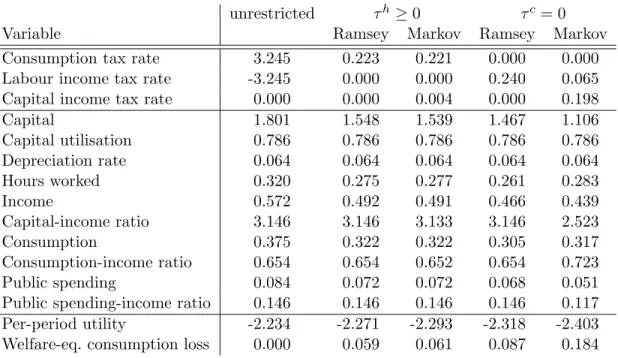
Table 2 shows the allocations and the tax rates at steady state for five policy models. The first column shows the case where the policy-maker has access to all three taxes and the tax rates are unrestricted. Remember that here both Ramsey and Markov policies can implement the first-best steady state. However, the tax rates seem unrealistic, with a consumption tax of 324.5 percent and a labour income tax of -324.5 percent.

Table 2: Tax rates and allocations at steady state

unrestricted τh ≥0 τc= 0

Variable Ramsey Markov Ramsey Markov

Consumption tax rate 3.245 0.223 0.221 0.000 0.000 Labour income tax rate -3.245 0.000 0.000 0.240 0.065 Capital income tax rate 0.000 0.000 0.004 0.000 0.198

Capital 1.801 1.548 1.539 1.467 1.106 Capital utilisation 0.786 0.786 0.786 0.786 0.786 Depreciation rate 0.064 0.064 0.064 0.064 0.064 Hours worked 0.320 0.275 0.277 0.261 0.283 Income 0.572 0.492 0.491 0.466 0.439 Capital-income ratio 3.146 3.146 3.133 3.146 2.523 Consumption 0.375 0.322 0.322 0.305 0.317 Consumption-income ratio 0.654 0.654 0.652 0.654 0.723 Public spending 0.084 0.072 0.072 0.068 0.051 Public spending-income ratio 0.146 0.146 0.146 0.146 0.117 Per-period utility -2.234 -2.271 -2.293 -2.318 -2.403 Welfare-eq. consumption loss 0.000 0.059 0.061 0.087 0.184

Columns 2 and 3 show the case where the government is prohibited from subsidising labour income. In this case, the Ramsey policy-maker (Column 2) taxes consumption at

14_{The derivatives of next period’s policy functions are computed using the Compecon Matlab package by}

Fackler and Miranda(2004).

22.3 percent at the steady state and sets the labour and capital income taxes to zero.16 The time-consistent policy-maker (Column 3) finances government spending mainly from taxing consumption as well, taxing it at 22.1 percent, and sets the capital income tax to 0.4 percent and the labour income tax to zero. Once a labour subsidy is ruled out, it is inefficient to tax both labour and consumption as both taxes distort the same margin, the consumption-leisure decision of the household. Optimal policy generally calls for using the less distortive tax (here the consumption tax) and sets the other (here the labour income tax) to zero. On this point, it is important to stress that there are several reasons for which taxing consumption is less distortive than taxing labour. The Laffer curve of the consumption tax peaks at infinity. This means that the loss of efficiency that this tax brings about is always less than proportional to its increase. This is not the case for the labour income tax, as its Laffer curve always peaks for τh ∈ (0,1). Moreover, as formally proved in Correia (2010), any revenue-neutral policy that increases consumption taxation and decreases labour income tax, the latter constrained to be non-negative, increases efficiency and therefore welfare.

Without consumption taxation, the Ramsey policy-maker (Column 4) taxes only labour income at the steady state, as is well known, while the time-consistent policy-maker (Col-umn 5) sets the labour income tax to 6.5 percent and the capital income tax to 19.8 percent. Hence, the most striking feature of the steady-state results is that with consumption taxation the Ramsey and Markov policies and allocations are very similar, unlike with only labour and capital income taxation.

Turning now to the allocations at steady state, note first that the consumption-income ratio and the public spending-income ratio are the same at the first best and at the Ramsey steady states. This is due to log utility, see Motta and Rossi (2014). Without consumption taxation, the time-consistent policies imply a significantly lower long-run capital-income ratio, a higher consumption-income ratio, a lower public spending-income ratio compared to the Ramsey case, which are all due to more distortions caused by taxation. The result that the public spending-income ratio is lower under Markov policy was first noted by Klein, Krusell, and R´ıos-Rull (2008) in an environment where only labour income taxes are available. Here we show that the same result holds in a scenario with both capital and labour income taxes. Finally, hours worked are higher under discretion than under commitment, because of the lower labour income tax.

Instead, with consumption taxation, as a result of less distortion caused by the need to raise fiscal revenue, the steady-state level of capital and income are higher. Notably, they are higher without commitment but with consumption taxation than under Ramsey policy but

16_{Note that the fact that the Ramsey policy-maker sets the consumption tax rate equal toα}

gwhenτh≥0

taxing only labour and capital income. Further, while it is still true that the capital- and public spending-income ratios are lower and the consumption-income ratio is higher under Markov than under Ramsey policies, all ratios change very little as a result of the change in commitment.

Table 2also shows the per-period utilities and the welfare-equivalent consumption losses compared to the first best at the steady state in the different taxation and commitment scenarios. With access to consumption taxation but imposing a non-negativity constraint on the labour income tax rate, the steady-state welfare loss amounts to 6.1 percent in the case of time-consistent policy, and 5.9 percent in the case of Ramsey policy-making. Without taxing consumption, the steady-state welfare-equivalent consumption loss is 18.4 percent under Markov-perfect policy, and 8.7 percent under Ramsey policy. Three results are worth stressing. First, taxing consumption generates larger welfare gains under discretion (66.9 percent) than under commitment (32.6 percent). Second, the welfare gains from commitment are small with consumption taxation (2.9 percent) and large without consumption taxation (52.4 percent). Third, welfare is higher without commitment but with access to consumption taxation than with commitment but taxing only labour and capital income.

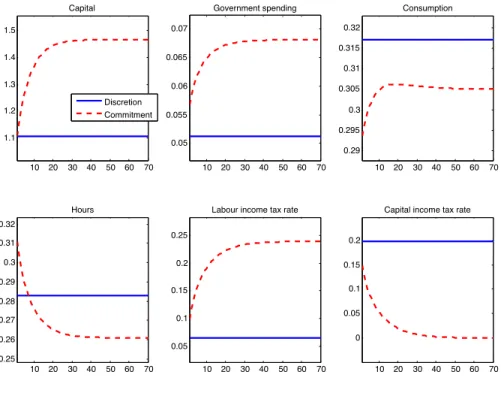
In order to get a sense of policy dynamics, we perform the following policy exercise. We assume that initially the economy is at the Markov steady state. At time zero a new policy-maker enters into office. She can either be a Markov policy-maker, in which case the same policies and allocations will be implemented in all periods t > 0, or have access to a commitment technology, in which case the economy will converge to the Ramsey steady state. Figures 1 and 2 show the dynamics of the allocations and the tax rates when the policy-maker does not have access to consumption taxation and when consumption is taxed but labour income cannot be subsidised, respectively.

Consider first the case with only labour and capital income taxation. At time 0, the Ramsey policy-maker sets capital taxes positive, since capital is a relatively inelastic tax base. However, as discussed above, capital income taxes distort the intratemporal margin of capital utilisation, hence it is sub-optimal to tax capital income at a high rate in period 0. During the transition, capital income taxes converge to zero. By reducing the capital income tax in any period t, the policy-maker positively affects capital accumulation in all previous periods, i.e., the downward trend in τk _{induces the household to continuously postpone her} consumption. At the same time, the Ramsey planner increases the labour income tax rate. This tax hike reduces labour supply in period t, but raises it in any previous period. Along the transition, capital, consumption, and government spending increase, while hours worked decrease.

the private sector’s behaviour in any previous period. This means that the time-consistent policy-maker does not internalise the benefits of a tax hike on labour income and a reduction in the capital income tax rate in terms of allocations in earlier periods. Furthermore, given the presence of endogenous capital utilisation and labour supply, both labour and capital income taxes are distortive within the period, while the capital tax distorts the Euler equation as well. In an attempt to minimise distortions the Markov policy-maker taxes both capital and labour income in the long run. In our baseline calibration, the long-run level of τk _{is higher} than τh_.

The possibility of taxing consumption changes markedly the features of optimal policy. Under commitment, the policy-maker sets the consumption tax rate positive and almost constant, avoids taxing labour income, and taxes capital income only initially, and even then at a very low rate. The policy-maker does not promise a tax hike on τc as doing so would be equivalent, via the Euler equation, to an increase in τk in the following period. This is suboptimal as the household would anticipate her consumption, leading to inefficiently low capital accumulation. Ceteris paribus, it is also suboptimal for the policy-maker to commit to a downward trend inτc_{, as this would provide an incentive to the household to inefficiently} increase labour supply during the transition. These two effects keep consumption taxes close to constant along the transition.

Given the low incentive to tax capital in the initial period, the time-inconsistency feature of Ramsey policies under consumption taxation is very limited compared to the standard case where the fiscal authority has access to labour and capital income taxation only. As a result, the tax policy functions under commitment and discretion are remarkably similar. Firstly, under Markov policy-making as well, it is suboptimal to jointly tax labour and consumption as these two taxes impact on the same intratemporal margin. Therefore, in the discretionary equilibrium as well, the labour income tax is zero at all times. Secondly, the Markov policy-maker recognises that present consumption taxation has a beneficial effect on today’s saving rate. At the same time, taxing capital distorts capital utilisation and, unlike a constant consumption tax, it also distorts the long-run Euler equation. In particular, by depressing the current saving rate, it would limit the amount of resources available to future generations. Therefore, despite capital being a relative inelastic source of revenue within the period, the time-consistent policy-maker taxes mainly consumption. Given that this policy is very similar to the one implemented by the Ramsey planner, the resulting time-consistent allocations are also very close to the Ramsey ones along the transition as well.

We can now compute the welfare gains from taxing consumption and from commitment taking into account the transition. First, we compute the gains from taxing consumption given a time-consistent policy-maker, starting from the Markov steady state without

con-sumption taxation. We find that the welfare gains in terms of welfare-equivalent consump-tion are 2.77 percent. Second, we perform the same calculation for a Ramsey policy-maker, starting from the Ramsey steady state without consumption taxation. Now the welfare gains from taxing consumption are 1.21 percent. Hence, the welfare gains from taxing consumption are much larger under discretion than under commitment.

Next, we compute the welfare gains from commitment both with and without consump-tion taxaconsump-tion, starting from the corresponding Markov steady state. We find that the welfare gains from commitment in terms of welfare-equivalent consumption are 0.0003 percent with consumption taxation and 2.01 percent with taxing labour income instead. Hence, the gains from commitment are negligible with access to consumption taxation, while they are sub-stantial without.

Finally, we can also compute the welfare gains from the different taxation and commitment scenarios compared to the existing tax system. We assume that initially the economy is at the actual steady state, described in Section 4.1. At time 0 a new policy-maker enters into office. She can be either a Markov or a Ramsey policy-maker, and with either access to consumption taxation or no access. In the case of a Ramsey policy-maker, the welfare gains are 7.745 percent and 7.06 percent with and without taxing consumption, respectively. Ceteris paribus, in the case of a Markov policy-maker, the welfare gains are 7.744 percent and 4.92 percent, respectively. Notice that the welfare gains are larger with consumption taxation and without commitment than without consumption taxation and with commitment. Table3

summarises our welfare results including transitions.

Table 3: Welfare gains in welfare-equivalent consumption units (percent)

Welfare gains... With cons. tax Without cons. tax ...from commitment 0.0003 2.01

...compared to the existing tax system ...from taxing consumption Ramsey 7.745 7.06 2.21

Markov 7.744 4.92 2.77

Figures 3 and 4 show the dynamics of the allocations and the tax rates without and with access to consumption taxation, respectively, for both a Ramsey and a time-consistent policy-maker. With access to consumption taxation, the whole dynamic path of taxes and allocations hardly differ with and without commitment.

4.4

Results with aggregate productivity shocks

We now study the cyclical properties of the policy instruments and allocations under the different tax and commitment scenarios. For each policy scenario, we simulate the model

and calculate sample statistics from the simulated data.17 The results of this exercise are reported in Table 4.

When consumption taxes are not available and the policy-maker can credibly commit (Column 3), the burden of taxation is almost entirely given to labour taxation. At the same time, labour income taxes hardly move in response to shocks, as the policy-maker prefers to use capital income taxes and public expenditure as shock absorbers. This is the well-known labour tax smoothing result of the Ramsey literature (Chari, Christiano, and Kehoe,1994). On the other hand, under discretion (Column 4 of Table4), the policy-maker uses both capital and labour income taxes in response to unexpected productivity changes. The coeffi-cient of variation of labour income taxation is more than three times larger and the coefficoeffi-cient of variation of capital income tax is more than a thousand times smaller than their Ramsey counterparts. This is mainly due to the fact that the Markov policy-maker is constrained to absorb a shock within the period, as any attempt to smooth the effects of random productiv-ity events via future taxation would not be credible. In our numerical example, the coefficient of variation of the capital income tax rate is roughly three-fifths of the coefficient of variation of labour taxes. Interestingly, the volatility of output and hours worked are slightly higher under commitment than under discretion, while the opposite is true for private and public consumption. Finally, both tax rates are countercyclical. These patterns are, for the most part, very similar to the ones presented in Klein and R´ıos-Rull (2003) and in Debortoli and Nunes (2010), although the class of economies they look at is slightly different.18

The differences between Ramsey and Markov policies are greatly reduced when the policy-maker can tax consumption (Columns 1 and 2 in Table4). Hence, the close similarity between Ramsey and Markov policy-making when consumption taxes are available extend to the cycli-cal properties of the stochastic allocation. As in the case without consumption taxation, the coefficient of variation of capital income taxes is larger than that of the alternative tax in-strument, in this case, the consumption tax. However, unlike without consumption taxation, without commitment capital taxes still play the main role in absorbing shocks. A new fea-ture of tax policies with consumption taxation is that the consumption tax rate is highly procyclical. The capital income tax rate remains countercyclical, but its correlation with output increases when consumption is taxed. All allocation variables, namely, consumption, public spending, hours, and output vary less with consumption taxation than without.

17_{We proceed as follows. We assume that in the initial period the system is in its stochastic steady state.}

We simulate the model for 1000 periods, using the same shocks across policy scenarios, and compute sample statistics. Finally, we take the median values of the sample statistics over 101 repetitions.

18_{In particular, Klein and R´ıos-Rull(2003) study a model with full capital utilisation, exogenous}

govern-ment spending and a capital income tax which is determined one or more periods in advance, whileDebortoli and Nunes (2010) consider a utility function with variable Frisch elasticity of labour supply.

Table 4: Cyclical properties of taxes and allocations

τh ≥0 τc= 0

Ramsey Markov Ramsey Markov Consumption tax Labour income tax

Mean 0.221 0.221 0.240 0.065

Standard deviation 0.005 0.005 0.002 0.002 Coefficient of variation 0.024 0.022 0.009 0.030 Autocorrelation 0.590 0.621 0.922 0.494 Correlation with output 0.9998 0.996 -0.700 -0.860 Capital income tax

Mean 0.000 0.004 0.000 0.198

Standard deviation 0.009 0.008 0.009 0.004 Coefficient of variation 10.483 1.894 30.693 0.019 Autocorrelation 0.590 0.618 0.463 0.490 Correlation with output -0.9995 -0.997 -0.801 -0.913 Public spending

Mean 0.072 0.072 0.068 0.051

Standard deviation 0.001 0.001 0.001 0.001 Coefficient of variation 0.015 0.015 0.019 0.022 Autocorrelation 0.974 0.976 0.775 0.799 Correlation with output 0.382 0.414 0.880 0.886 Public spending-income ratio

Mean 0.146 0.146 0.146 0.117

Standard deviation 0.005 0.004 0.004 0.003 Coefficient of variation 0.031 0.030 0.026 0.023 Autocorrelation 0.508 0.511 0.514 0.490 Correlation with output -0.899 -0.898 -0.936 -0.892 Consumption

Mean 0.322 0.322 0.305 0.317

Standard deviation 0.005 0.005 0.005 0.006 Coefficient of variation 0.015 0.015 0.017 0.018 Autocorrelation 0.974 0.976 0.939 0.934 Correlation with output 0.382 0.414 0.621 0.665 Hours

Mean 0.275 0.276 0.260 0.283

Standard deviation 0.006 0.006 0.007 0.007 Coefficient of variation 0.021 0.020 0.027 0.025 Autocorrelation 0.512 0.515 0.513 0.490 Correlation with output 0.866 0.864 0.937 0.901 Output

Mean 0.493 0.492 0.467 0.439

Standard deviation 0.017 0.016 0.020 0.018 Coefficient of variation 0.034 0.033 0.042 0.040 Autocorrelation 0.585 0.588 0.570 0.578 Welfare-eq. consumption loss 0.059 0.061 0.087 0.183

Finally, we compute long-run expected welfare as a percentage increase in welfare-equivalent consumption units in all periods and all states in a particular policy scenario that is neces-sary to make the representative household as well off as at the first best.19 _{The values we}

find are very similar to those for the deterministic steady state, and hence our main conclu-sions extend to the stochastic environment, namely, that (i) taxing consumption generates larger welfare gains under discretion than under commitment, and (ii) the welfare gains from commitment are small with consumption taxation and large without consumption taxation. Therefore, the business cycle results confirm the similarities between Ramsey and Markov equilibria when the policy-maker has access to consumption taxation, as well as the welfare benefits of taxing consumption.

4.5

Robustness checks

In this section, we show that our results are robust to changing some parameter values and to using different solution algorithms. First of all, we consider a wide range of values for the Frisch elasticity of labour supply without productivity shocks. In particular, we consider (i) ϕ = 0.4, which is in line with recent micro estimates such as Domeij and Floden (2006) (see also Guner, Kaygusuz, and Ventura, 2012), (ii) ϕ = 1, which is often chosen in the macro literature (e.g. Christiano, Eichenbaum, and Evans, 2005), and (iii) ϕ= 5 as a high value, which is sometimes chosen to better match the intertemporal variation of aggregate hours (e.g.Gal´ı, L´opez-Salido, and Vall´es,2007). We adjustα` appropriately in each case as described in Section 4.1.

The first three panels of Table 5 show that the steady-state results are only marginally affected by changingϕ, except in the case of a time-consistent policy-maker without access to consumption taxation (last column of Table 5). For all values ofϕwe consider, the Ramsey planner finances all public expenditure with either only labour income or only consumption taxation. Under discretion, the changes in tax rates are very small if consumption taxation is available. On the other hand, we find large differences when consumption taxes are not available. In that case, τh varies from 17.3 to 4.2 percent and τk from 7.8 to 22.1 percent as

ϕ increases. This is because increasing the elasticity of labour supply increases the relative distortion of τh compared to τk. As a result, the optimal time-consistent policy calls for lower labour income tax rates and higher capital income tax rates.

Increasing the Frisch elasticity increases the welfare losses under all policy scenarios.

19_{In order to do this, for some percentage increase in consumption ε, we simulate the economy over 600}

periods, compute per-period utility for the last 500 periods, and finally take the average over 501 such simulations. Then we find theεsuch that the average per-period utility matches the one found for the first best from similar simulations.

This is because, ceteris paribus, a higher ϕimplies a stronger response of hours to any given distortion of the consumption-leisure margin. It is also worth noticing that under discretion as ϕ gets bigger, the public spending-income ratio decreases. This is because the Markov planner decides to have lower steady-state taxes as the distortionary effects of fiscal policy are greater. These effects are almost absent in the case with consumption taxation. Increasing the Frisch elasticity does not remove the policy-maker’s incentive to give almost all the burden of taxation to consumption and to keep the public spending-income ratio every close to its efficient level.

Afterwards, we increase the coefficient of relative risk aversion to 2, i.e., now the current utility function is u(c, `, g) = c 1−σ<sub>−1</sub> 1−σ −α` (1−`)1+1/ϕ 1 +1_/ϕ +αg g1−σ−1 1−σ ,

with σ = 2 and ϕ = 3. We recalibrate the utility weights α` = 16.791 and αg = 0.050 to keep hours at 0.249 andg_{/y at 0.155 before the reform. The results are in the fourth panel of} Table 5. Our conclusions remain unaltered.

In the fifth panel of Table5, we report the steady-state results for the case where we keep

σ = 1 and ϕ = 3 but set β = 0.96, the most-commonly used value in the macro literature for yearly models. Again our results are not affected.

Then, we set χ = 1.8 and adjust η = 0.098 so that the capital utilisation rate at the steady state be the same as in the data. Note that this implies a depreciation rate of 0.076 at the steady state. Panel 6 of Table 5shows that our conclusions do not change.

We also consider a higher value ofαg, 0.3 in particular, while keeping all other parameters at their baseline values. In this case the consumption tax base is smaller as a share of GDP than in the baseline calibration. The results are in Panel 7 of Table 5. Ramsey and Markov policies and allocations are very similar with consumption taxation in this case as well.

Remarkably, under all parameterisations considered, taxing consumption is more impor-tant than being able to commit. As reported in Tables 2 and 5, welfare is always higher under Markov policy-making and consumption taxation than under Ramsey without taxing consumption.

We solve the stochastic model as well with ϕ = 1 to check the robustness of the cycli-cal properties of tax rates and allocations. Table 6 shows that the main features remain unchanged.

Finally, we also check the robustness of our results to using different numerical algorithms. In particular, using the solution to the Ramsey problem by policy function iteration as initial guess, we solve it again parameterising the policy functions using Chebyshev polynomials or cubic splines. Then, we solve the time-consistent policy-maker’s problem by parameterising

the policy functions again. In this second solution algorithm we iterate until the parameters of the policy functions converge. The resulting tax rates and allocations are identical up to many decimals to the ones computed using policy function iteration.

5

Concluding remarks

This paper has studied the properties of time-consistent optimal fiscal policies when the policy-maker has access to consumption taxation, both in a deterministic setting and over the business cycle. Contrary to the case with only labour and capital income taxation, time-consistent policies, and hence allocations, are very close to those under Ramsey policy, as long as capital income taxation causes some distortion within the period. This also means that the Ramsey policies are close to time-consistent in the sense that if a new policy-maker with the same objective entered in a randomly chosen period or due to the electoral cycle, policies would hardly change. Further, in a deterministic setting, a close-to-constant consumption tax rate is enough, and we do not have to rely on a rich structure of public debt, as in Zhu

(1995) and Dom´ınguez (2007).

When the labour income tax rate is restricted to be non-negative, the optimal time-consistent capital income tax rate is close to zero (0.4 percent), the consumption tax rate is 22.1 percent, and labour income is not taxed at the steady state. The proposed time-consistent policies with consumption taxation would yield welfare gains of 7.744 percent in terms of welfare-equivalent consumption units compared to the existing tax system, taking into account the transition. These welfare gains are almost as large as under commitment (7.745 percent), and are larger than the gains a Ramsey policy-maker could achieve without access to consumption taxation (7.06 percent). If the time-consistent policy maker can only tax labour and capital income, the welfare gains are reduced to 4.92 percent.

In this paper we have considered a representative-agent framework, hence we studied the optimal tax mix from an efficiency perspective only, to raise fiscal revenue. An important task for future research is to analyse the distributional impact of the different tax instruments in a model with heterogeneity across households.

References

Azzimonti, M., P.-D. Sarte, and J. Soares (2009). Distortionary Taxes and Public Investment when Government Promises are not Enforceable. Journal of Economic Dynamics and Control 33(9), 1662–1681.

Chari, V. V., L. J. Christiano, and P. J. Kehoe (1994). Optimal Fiscal Policy in a Business Cycle Model. Journal of Political Economy 102(4), 617–652.

Christiano, L. J., M. Eichenbaum, and C. L. Evans (2005). Nominal Rigidities and the Dynamic Effects of a Shock to Monetary Policy. Journal of Political Economy 113(1), 1–45.

Coleman, W. J. I. (2000). Welfare and Optimum Dynamic Taxation of Consumption and Income. Journal of Public Economics 76(1), 1–39.

Correia, I. (2010). Consumption Taxes and Redistribution. American Economic Re-view 100(4), 1673–1694.

Correia, I., E. Farhi, J. P. Nicolini, and P. Teles (2013). Unconventional Fiscal Policy at the Zero Bound. American Economic Review 103(4), 1172–1211.

Debortoli, D. and R. Nunes (2010). Fiscal Policy under Loose Commitment. Journal of Economic Theory 145(3), 1005–1032.

Domeij, D. and M. Floden (2006). The Labor-Supply Elasticity and Borrowing Constraints: Why Estimates are Biased. Review of Economic Dynamics 9(2), 242–262.

Dom´ınguez, B. (2007). On the Time-Consistency of Optimal Capital Taxes. Journal of Monetary Economics 54(3), 686–705.

Fackler, P. and M. Miranda (2004). Applied Computational Economics and Finance. The MIT Press.

Farhi, E., G. Gopinath, and O. Itskhoki (2014). Fiscal Devaluations. Review of Economic Studies 81(2), 725–760.

Gal´ı, J., J. D. L´opez-Salido, and J. Vall´es (2007). Understanding the Effects of Government Spending on Consumption. Journal of the European Economic Association 5(1), 227–270.

Greenwood, J., Z. Hercowitz, and G. W. Huffman (1988). Investment, Capacity Utilization, and the Real Business Cycle. American Economic Review 78(3), 402–417.

Greenwood, J., Z. Hercowitz, and P. Krusell (2000). The role of investment-specific techno-logical change in the business cycle. European Economic Review 44(1), 91–115.

Guner, N., R. Kaygusuz, and G. Ventura (2012). Taxation and Household Labour Supply.

Review of Economic Studies 79(3), 1113–1149.

Klein, P., P. Krusell, and J.-V. R´ıos-Rull (2008). Time-Consistent Public Policy. Review of Economic Studies 75(3), 789–808.

Klein, P. and J.-V. R´ıos-Rull (2003). Time-Consistent Optimal Fiscal Policy. International Economic Review 44(4), 1217–1245.

Lansing, K. J. (1999). Optimal Redistributive Capital Taxation in a Neoclassical Growth Model. Journal of Public Economics 73(3), 423–453.

Marcet, A. and R. Marimon (2011). Recursive Contracts. Mimeo.

Martin, F. M. (2010). Markov-perfect Capital and Labor Taxes. Journal of Economic Dynamics and Control 34(3), 503–521.

Mertens, K. and M. O. Ravn (2011). Understanding the Aggregate Effects of Anticipated and Unanticipated Tax Policy Shocks. Review of Economic Dynamics 14(1), 27–54.

Motta, G. and R. Rossi (2014). Ramsey Monetary and Fiscal Policy: the Role of Consumption Taxation. Mimeo.

Ortigueira, S. (2006). Markov-Perfect Optimal Taxation. Review of Economic Dynam-ics 9(1), 153–178.

Straub, L. and I. Werning (2014). Positive Long Run Capital Taxation: Chamley-Judd Revisited. Working Paper 20441, National Bureau of Economic Research.

Tauchen, G. (1986). Finite State Markov-chain Approximations to Univariate and Vector Autoregressions. Economics Letters 20(2), 177–181.

Trabandt, M. and H. Uhlig (2011). The Laffer Curve Revisited. Journal of Monetary Eco-nomics 58(4), 305–327.

Trabandt, M. and H. Uhlig (2012). How Do Laffer Curves Differ across Countries? NBER Working Papers 17862, National Bureau of Economic Research.

Zhu, X. (1995). Endogenous Capital Utilization, Investor’s Effort, and Optimal Fiscal Policy.

Appendices

A

First-best allocation

The first best allocation can be found by maximising the following Lagrangian:

max {ct,`t,ht,gt,kt+1,vt}∞t=0 E0 ( <sub>∞</sub> X t=0 βt[u(ct, `t, gt) +λ1,t(1−`t−ht) +λ2,t at(vtkt)γh1 −γ t + (1−δ(vt))kt−ct−gt−kt+1 ,

where we have used (9) to replace for yt in (12). The first-order conditions with respect to

ct, `t, ht, gt, kt+1, ut, λ1,t, and λ2,t are uc,t = λ2,t (30) u`,t = λ1,t (31) at(1−γ) vtkt ht γ = λ1,t (32) ug,t = λ2,t (33) λ2,t = βEt " λ1,t+1 at+1γv γ t+1 ht+1 kt+1 1−γ + 1−δ(vt+1) !# (34) δu,t = atγ ht vtkt 1−γ , (35) `t+ht = 1 (36) ct+gt+kt+1 = at(vtkt) γ h1_t−γ+ (1−δ(vt))kt (37)

Straightforward combinations of (30)-(37) lead to the following equations which characterise the first-best allocation:

ug,t = uc,t, ∀t, (38) u`,t uc,t = at(1−γ) vtkt ht γ , ∀t, (39) ht+`t = 1, ∀t, (40) uc,t = βEt " uc,t+1 1−δ(vt+1) +at+1γvt+1 ht+1 vt+1kt+1 1−γ!# , ∀t, (41) ct+gt+kt+1 = at(vtkt)γh1t−γ+ (1−δ(vt))kt, ∀t, (42) δv,t = atγ ht vtkt 1−γ , ∀t, (43)

B

First-order conditions of the policy problems

We assume that the utility function is separable with respect to its three arguments, hence the second cross-derivatives are zero.

B.1

First-order conditions of the Ramsey policy-maker’s problem

The first-order conditions with respect toτc_{, c, `, h, g, k}0_{, v, andλ}

1, λ2, λ03, λ4, λ5, respectively, are 0 = 1 (1 +τc₎2 " −λ0₃uc+λ3uc 1−δ(v) +av h vk 1−γ − g−τ c_c k ! −λ5(1−γ)a vk h γ −λ4 c vk − u` uc h vk −λ3 uc 1 +τc c k (44) 0 =uc−λ2+λ03 ucc 1 +τc −λ3 ucc 1 +τc 1−δ(v) +av h vk 1−γ − g−τ c<sub>c</sub> k ! −λ3 uc 1 +τc τc k −λ4 τc vk + u` u2 c ucc(1 +τc) h vk +λ5 u` u2 c ucc (45) 0 =u`−λ1 +λ3u`` h k +λ4 u`` uc (1 +τc) h vk −λ5 u`` uc (46) 0 =−λ1+λ2a(1−γ) vk h γ −λ3 uc 1 +τca(1−γ) vγ hγ_k1−γ − u` k −λ4 a(1−γ)h−γ(vk)γ−1− u` uc (1 +τc) 1 vk −λ5 1 1 +τcaγ(1−γ) (vk) γ h−γ−1 (47) 0 =ug −λ2+λ3 uc 1 +τc 1 k +λ4 1 vk (48) 0 =−λ2+βE ( λ0₂ a0v0γγ h0 k0 1−γ + 1−δ(v0) ! +λ0₃ u0_c 1 +τc0 a0v0γ(1−γ)k0γ−2h01−γ− g 0_−τc0_c0 k02 −u0_{`</sub>h 0 k02 (49) +λ0<sub>4</sub> a0(1−γ)k0γ−2 h0 v0 1−γ − g 0<sub>−τ</sub>c0<sub>c</sub>0 v0<sub>k</sub>02 − u0<sub>`} u0 c (1 +τc0) h 0 v0_k02 ! +λ0₅ 1 1 +τc0a 0 (1−γ)γ v 0γ k01−γ_h0γ

0 =λ2 aγvγ−1kγh1−γ−δvk +λ3 uc 1 +τc δv−aγv γ−1 h k 1−γ! +λ4 a(1−γ)vγ−2 h k 1−γ − g−τ c_c v2_k − u` uc (1 +τc) h v2<sub>k</sub> +δvv ! (50) +λ5 1 1 +τca(1−γ)γv γ−1 k h γ 0 =`+h−1 (51) 0 =c+g+kt+1−a(vk)γh1−γ−(1−δ(v))k (52) 0 =− uc 1 +τc +βE " u0_c 1 +τc0 1−δ(v 0 ) +a0v0 h0 v0_k0 1−γ −g 0 _−τc0_c0 k0 ! −u0<sub>`</sub>h 0 k0 # (53) 0 =a h vk 1−γ −g−τ c<sub>c</sub> vk − u` uc (1 +τc) h vk −δv (54) 0≥ u` uc − 1 1 +τca(1−γ) vk h γ , (55)

λ5 ≥0, with complementary slackness condition, andλ3,−1 = 0.

B.2

First-order conditions of the time-consistent policy-maker’s

problem

The first-order conditions with respect to τc_{, c, `, h, g, k}0_{, v, respectively, are}

0 =−λ3 1 (1 +τc₎