A Load Balancing Schema for Agent-based SPMD Applications

A Load Balancing Schema for Agent-based SPMD Applications

Claudio Márquez, Eduardo César, and Joan Sorribes

Computer Architecture and Operating Systems Department (CAOS),

Universitat Autònoma de Barcelona, 08193 Bellaterra, Spain

Email: [email protected], {eduardo.cesar,joan.sorribes}@uab.cat

simulations of complex systems. When large number of agents and complex interaction rules are required, an HPC infrastructure can be helpful for executing such simulations in a reasonable time. However, complex interaction rules usually cause workload imbalances that negatively affect the simulation time. In this paper, we propose a load balancing schema that tries to find a reduced combination of exchanges to balance the computing time of the processes. The method adjusts the computational load within a certain range of tolerance, computing the global reconfiguration of the work-load using computing time, and the number of agents. Experiments show gains between 15 and 30 percent of the Execution time. In addition, we propose a modification of the agent-based simulation framework named FLAME that provides the automatic generation of the routines needed to dynamically migrate agents among different computational units.

Keywords: Agent-based Simulation, FLAME, Load Balancing, Application Tuning, SPMD.

1. Introduction

Agent-Based Modeling and Simulations (ABMS) can take advantage of High Performance Computing (HPC) systems. Generally, HPC systems facilitate the execution of more realistic scenarios with many agents and complex interaction rules. Moreover, when the simulation requires more com-putational scalability, SPMD paradigm is commonly used. These SPMD applications execute the same program in all processes, but with a different set of the domain.

ABMS show significant variations in amount of comput-ing and communication times. Durcomput-ing the simulation process load imbalances are likely to appear due to the high-level of interaction between agents and the different rules of behavior exhibited by most of these models. In addition, an unequal distribution of agents causes load imbalances that negatively affect the execution time of the simulation.

In order to solve such problems, the parallel SPMD simulation environments should include a dynamic load balancing mechanisms that allows the migration of agents between different computational units.

This paper is addressed to the PDPTA’13 Conference

Currently, few parallel ABMS environment oriented to HPC environments can be found. Ecolab [1] is an object ori-ented environment written in C++ and MPI. Repast HPC [2] was recently released in 2012, it is also written in C++ using MPI for parallel operations. Contrary to Ecolab, Repast HPC was created from the beginning for large-scale distributed computing platforms. Although both Ecolab and Repast HPC argue that agents should be migrated; they do not include generic migration routines, so the developer should implement the whole migration code. Finally, FLAME [3] allows the production of automatic parallelizable code to run on large HPC system.

Dynamic load balancing strategies are commonly de-veloped using centralized or hierarchical approaches. Un-fortunately, these approaches report a high computational cost and scalability problems. In other hand, decentralized approaches can present problems regarding the quality of the balance because the neighboring processes exchange incomplete information. In [4] is proposed a centralized load balancing based on space repartitioning. In [5] a hierar-chical multi-level load balancing strategy is presented, and centralized and hierarchical schemas are compared. In [6] three algorithms using recursive domain decomposition in a binary tree structure are compared using balance speed and communication costs. In [7] a complex partitioning approach based on irregular spatial decompositions is presented. In [8] and [9] distributed cluster-based partitioning and load balancing schema for problems of flocking behaviors are defined.

In general, most of ABMS platforms do not include a load balancing mechanism, and usually the strategy depends on the nature of the agent model. Moreover, the load balancing studies take place usually in non-SPMD platforms, and most of them use applications created with integrated strategies. Consequently, we decided to develop a strategy independent platform, and integrate it in FLAME as a plugging. This plat-form has been continuously developed from 2006. FLAME is written in C using MPI and is aimed principally at the economical, medical, biological and social science domains. The code generated by FLAME lacks the necessary routines to allow the migration of agents. Therefore, before using any Load Balancing schema, a migration mechanism should be implemented.

This paper describes a Load Balancing schema and a modification of the FLAME framework that provides the

automatic generation of the routines needed to migrate agents between different computational units. Using these routines, our Load Balancing schema allows automatic and dynamic tuning decisions in terms of computational load.

The rest of this document is organized into five sec-tions. First, Section 2 briefly describes FLAME. Next, the proposed load balancing schema is discussed (3), then the migration routines are presented (4). The results section presents a comparison of the schema for two scenarios (5). The final section includes the conclusions (6).

2. FLAME

FLAME was developed at the University of Sheffield in collaborations with the Science and Technology Facilities Council (STFC) in the United Kingdom. FLAME can be used to solve problems involving multiple domains such as economical, medical, biological and social sciences. This framework allows writing several agents and non-agent models using a common simulation environment, and then performs simulations in a simple way on different parallel architectures, including GPUs.

2.1 General Overview

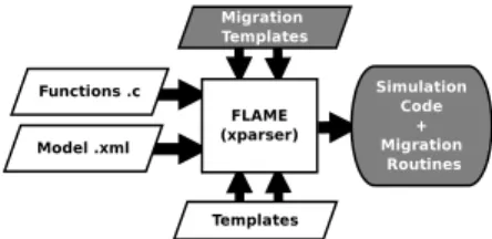
FLAME is not a simulator in itself, but a tool able to generate the necessary source code for the simulation. It automatically generates the simulation code in C through a template engine. FLAME provides a set of template files that the template engine uses to generate the simulation code getting information from the model specification. In the same way, the migration routines are automatically generated from a set of extra template files. The model specification is described by two types of files, XMML (X-Machine Markup Language) files, which is a dialect of XML, and the implementation of the agent functions contained in C files. Figure 1 shows the files required by FLAME to create the simulation code.

Fig. 1: Diagram of the FLAME framework. The functionality of FLAME is based on finite state machines called X-machines, which consists of a finite set of states, transitions between states, and actions. To perform the simulation, FLAME holds each agent as an X-machine data structure, whose state is changed via a set of transition functions. Furthermore, the transition functions perform message exchanges between agents if necessary. Then, the simulation environment is composed mainly of a set of X-machines defined through their state transitions, internal memory, and agent messages.

The transitions between the states of the agents are accomplished by keeping the X-machines in linked lists. The simulation environment has one linked list for each state of a specific agent. During the simulation, the X-machines are inserted into the list related to the initial state, later the corresponding transition function is applied to each X-machine. Afterwards, these X-machines are inserted in the list related to the next state. This process is repeated until the last state, which determines the end of the iteration.

2.2 Parallelization

In HPC environments, FLAME communications are man-aged by the Message Board Library libmboard, which uses MPI to communicate between processes. Libmboard

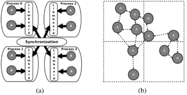
handles the agents messages through message managing mechanisms and filtering before being sent to local agents and agents belonging to external processes. FLAME handles deadlocks through synchronization points, which ensure that all the data is coordinated among agents using a Single Program Multiple Data (SPMD) pattern.

Figure 2(a) shows the communication between local agents and external agents usinglibmboardlibrary. Hence, this library sends all messages to the agents through a coor-dinated communication between different MPI processes.

(a) (b)

Fig. 2: Parallel communication and synchronization via libmboard (a). Workload problems associated with distri-bution of agents(b).

2.3 Distribution of the Agents

The parallel distribution of the agents in FLAME is based on two static partitioning methods: geometric partitioning and round-robin partitioning. Currently, FLAME does not include mechanisms to enable the movement of agents between processes. Thus, the workload in each process will rely on the evolution of the model from its initial population of agents. Consequently, evolution of the simulation may trigger computing problems causing overhead, and also may produce excessive external communications due to the interaction among agents (as shown in Figure 2(b)). Therefore, the time required to complete the simulation will be negatively affected.

3. Load Balancing Schema

In agent-based SPMD applications, estimation of perfor-mance is a difficult task. In many instances, the perforperfor-mance can vary by issues such as: amount of computation, interac-tion pattern between agents, and environmental influences. These issues depend on the complexity of the model, and whether the simulation model has different kinds of agents or not. In the same way, depending on the internal state of the agents, these issues can change during the simulation process. For this reason, this schema dynamically decides the global reconfiguration of the workload using an imbalance threshold, computing time, and the number of agents. The threshold is a value between 0 and 1 that represents the acceptable imbalance degree. Computing times and number of agents are monitored in each iteration during the simula-tion. This approach is executed by all the processes without a central unit of decision. Therefore, each process knows the global load situation and executes the algorithm with the same input. Consequently, all processes calculate the same reconfiguration of the workload.

The mechanism is triggered when an imbalance factor is detected outside the tolerance range. This factor indicates the percentage of imbalance in respect to the mean, and the tolerance range defines the permissible degree of imbalance (see algorithm 1). Moreover, it does not need to perform after an iteration has been finished. In order to get a better result, the load balancing mechanism should be executed between the transition phases inside an iteration. Our schema consists of the phases described below.

3.1 Monitoring

The schema is executed by all the processes; hence each process needs to know the global load situation. Thus, in each iteration, the computing time and the number of agents of all processes is broadcasted by a collective MPI communication. Our load balancing schema can be executed in each iteration of the simulation. However, depending on the complexity of the agent model, the migration process would have better result if used between the transition phases of the simulation. For this reason, before sharing the workload information, we have to determine the current computing time. Based on the results of a previous iteration, the current computing time predicts the computing time for the current number of agents before finalizing the current iteration. As described in Equation 1, the current computing time is predicted based on the current number of agents and the information of the previous iteration.

comp_timeiter=

comp_timeiter−1∗num_agentsiter

num_agentsiter−1

(1) This information is exchanged using a collective MPI call. Once all processes have the global workload information, the activation mechanism is checked.

Algorithm 1Global overview of the Load Balancing schema collect all computing times for each process

avg_time←P_{comp_time}

i/nprocs

ib_f actori ←comp_timei/avg_time

tolerance←threshold∗avg_time

if∀i∈procs,∃ proci/|imbalance(proci)|>tolerance

then

sort computing times in descending order

center←index of the less overloaded process

i←index of the first process in thesorted list j←index of the last process in thesorted list end if

while|imbalance(proci∧procj)|>tolerancedo

calculatecontribution_rangei

j←index of the last process in thesorted list while|imbalance(proci∧procj)|>tolerancedo

calculateacquisition_rangej

calculate expected migration forproci|procj

sort underloaded computing times fromcenter if|imbalance(proci)|₆tolerancethen

break

end if j− −

end while

sort overloaded computing times untilcenter i←index of the first process in thesorted list if|imbalance(proci)|6tolerancethen

break

end if end while

Execute the asynchronous exchanges

3.2 Activation Mechanism

In this phase, with the purpose of detecting imbalances, the imbalance factor and the permitted tolerance of im-balance are calculated for each process. The imim-balance factor represents the degree of imbalance according to the mean computing time. The tolerance allows setting the range where the execution is considered as balanced. Con-sequently, depending on this tolerance range, an imbalance can be detected (respectively, Equations 2 and 3 show the imbalance factor, tolerance and the tolerance range).

ib_f actori=

comp_timei

avg_time (2)

tolerance=avg_time∗threshold tolerance_range=avg_time±tolerance (3) The Load Balancing mechanisms is triggered if a com-puting time is detected outside of this tolerance range. Furthermore, as every process executes this analysis with

(a)

(b)

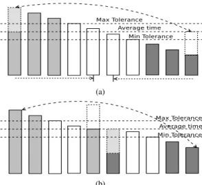
Fig. 3: Comparison and resorting in pairs.

the same inputs (times and agents of all processes), every process have same balanced and imbalanced processes.

3.3 Comparison procedure

In this step, the schema should decide how many agents need to be reallocated. This phase consists of performing comparisons between the most overloaded and the most underloaded processes. In order to reduce communication cost, the criterion of migration is defined by adjusting these processes inside the tolerance range during one exchange. This is explained in the next subsection.

First, our algorithm sorts the computing times per node by descending imbalance factor (Figure 3(a)). Then, following the criterion described in the next subsection, the number of agents that should be migrated for the first and the last process is determined. Therefore, the computing time of these processes will change by the expected time, which corresponds to the time for the expected configuration of agents. Once this is done, the next step consists of reordering by the expected imbalance factors after the migration. Then, first and last process will be changed as shown in Figures 3(a) and 3(b).

The load balancing procedure is repeated until all pro-cesses are in the tolerance range of balance.

3.4 Load Balancing Criterion

In this section, the criterion for calculating the expected migration agents between two processes is depicted. Due to the complex interaction rules of the agents, the computing time of one agent is not fixed. Therefore, doing a speculation of this time based on the current total of the agents in the simulation can be inaccurate. In order to ensure the balancing of the overloaded process, we consider calculating the number of agents to migrate according to the average time per agent of the sender process (overloaded process).

(a) (b)

Fig. 4: Examples of the expected migration.

(a) (b)

Fig. 5: Examples of the expected migration.

This algorithm tries to find a reduced combination of exchanges to balance the computing time of the processes. To begin with, the time required to reach the tolerance range of balancing is calculated by Equations 4 and 5 ( i and

j represent the most overloaded and underloaded process, respectively).

exceeded_timei=comp_timei−avg_time

contribution_rangei=exceeded_timei±tolerance (4)

required_timej=avg_time−comp_timej

acquisition_rangej=required_timej±tolerance (5)

In order to minimize the migration exchanges, the ex-pected number of agents to migrate should make both processes go If the sender process has more exceeded time than the required time for the receiver, then as shown in Figure 5(a), the exceeded time is split according to the ideal required time by the receiver. Subsequently, this procedure should be repeated over the next underloaded process until the entire exceeded time of the sender is reduced. In the other hand, if the sender process has not enough exceeded time to fill the required time of the receiver, then as shown in Figure 5(b), the full exceeded time of the sender is migrated. Likewise, this procedure should be repeated over the next overloaded process until the entire required time of the receiver is completed.

Consequently, based on the total time to be reallocated, the number of agents for the migration should be calculated. As noted above, we use the number of agents to migrate according to the average time per agent of the overloaded process because we consider that the overloaded process has priority for the global reduction of the computing time. This time is determined by the Equation 6 (i means the number rank of the overloaded process).

time_per_agenti=

comp_timei

num_agenti

Once all the movement of agents has been determined, the migration phase is triggered. During the next phase, the amount of agents defined by the criterion of load balancing is migrated.

4. Migration of Agents

With the final objective of introducing automatic load balancing strategies in HPC agent based systems, it is necessary to develop efficient agent migration mechanisms. Our proposal consists of automatically generating the agent migration code for FLAME through the same template structure used for generating the simulation code. In order to achieve this new feature, new templates for generating the migration routines are required. Then, the template engine processes these templates to obtain the information about the model and generates migration routines together with the simulation code (as shown in Figure 6).

Fig. 6: Diagram of the FLAME framework with the enhanc-ing.

Once the information about the agent has been obtained by the new templates, the migration routines can automatically add and remove agents in the migration process. This agents are held in output lists identified by the id of the target process. Later, the agents in the output listsare packed to be sent out. The received data is unpacked and later inserted with the others agents in the recipient process. Algorithms 2 and 3 show the procedures involved during the migration of agents.

With the purpose of sending the agents to a recipient process in a single communication, the agents in the lists need to be stored in contiguous memory.This migration is accomplished by packing and unpacking data using M P I

functions. These M P I functions require memory buffers before being used, which sizes depend on the type and amount of agents. Consequently, the generated migration routines automate calculations of the buffer sizes required during the migration process.

Algorithm 2 Sending Agents

whileagents to be sentdo

insert in therecipientlist

end while

calculate the sizes and create the buffers pack the agents and send the packages

Algorithm 3 Receiving Agents

create the memory buffers and receive the agents

whilepacked agentsdo

unpack and insert agent in the current process

end while

Before performing the migration process, a criterion must be established to decide which agents should be sent (as discussed in the previous section). Then, the migration process starts through the migration routines mentioned in section 4.1. The migration process should also require deciding when it should be performed. Nevertheless, this partially depends on the criterion by which the agents were selected.

4.1 Migration Routines

The migration routines are specifically generated for each type of agent in the model. In consequence, it is possible to perform migrations after any transition.

The following list introduces the main migration routines. In addition, the prefix NAME indicates the name of a specific type of agent.

• Init_movement: Initializes global variables and data structures involved in the migration.

• prepare_to_move_N AM E: Moves agents to a spe-cific output linked list and removes them from the current process.

• P ack_N AM E_agent_list: Packs all agents kept

in the output linked lists in contiguous memory (MPI_PACKED datatype), one for each recipient.

• U nP ack_N AM E_agent_list: Unpacks the packed

agents received as MPI_PACKED. Then, inserts the received agents in the X-machine list of the current process.

5. Experimental Results

The main objective of this section is to demonstrate that using the proposed load balancing schema and migration routines, it is possible to correct imbalance problems in an agent based SPMD application.

The example is a SIR epidemic model on a 2D toroidal space. The SIR model describes the spread of an epidemic within a population. The population is divided into three groups: the Susceptible (S), the Infectious (I), and the Recovered (R). For this reason, this model is called SIR. Summarizing, a susceptible individual is who is not infected and not immune, the infectious are those who are infected and can transmit the disease, and the recovered are those who have been infected and are immune. Additionally, natural births and deaths during the epidemic are included in this SIR model, so individuals might die from the disease or by natural death due to aging. Consequently, births and deaths represent a dynamic creation and elimination of

agents. Therefore, the workload can change as the simulation proceeds.

Table 1: Initial parameters for both scenarios.

Parameters values Parameters values

infected 10 infectiousness 65

lifespan 100 chance recovery 50

average offspring 4 disease duration 20

In this section, two scenarios are presented. Table 1 depicts the environmental configurations of the simulations. Both simulations are started with an initial population (see Table 2), and 10 of these are infected. The experiments were performed during 200 simulation steps and, the agents were distributed doing a round-robin distribution. Thus, depending on the number of processes and the initial agents, the initial number of agents per process can be equal or similar.

Table 2: Scenarios of the experiments.

scenario agents carrying capacity space dimensions

A 30000 30000 650X650

B 50000 50000 1000x1000

The Load Balancing schema is activated after the fifth simulation step. Given that the computing measurements vary when the migration process has been triggered, the activation mechanism is blocked during the next iteration. After this, the activation mechanism will be enabled again. Sending and receiving of the agents has been deployed using MPI asynchronous functions to overlap the costs of communication and computation.

The experiments were run using the FLAME Framework 0.16.2, libmboard 0.2.1 and OpenMPI 1.4.1. All experiments were executed on a Cluster IBM with the following features: 32 IBM x3550 Nodes, 2xDual-Core Intel(R) Xeon(R) CPU 5160 @ 3.00GHz 4MB L2 (2x2), 12 GB Fully Buffered DIMM 667 MHz, Hot-swap SAS Controller 160GB SATA Disk and Integrated dual Gigabit Ethernet. Additionally, we tested our schema using a case without Load Balanc-ing schema, and three imbalance tolerances: 0.3(30%) , 0.15(15%) and 0.05(5%). Moreover, for both scenarios, 16, 32, 64 and 128 cores were used.

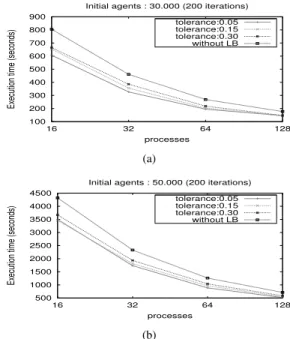
Figures 7(a) and 7(b) compare the execution time with varying number of processes by comparing different values of tolerance with the original simulation without the load balancing schema. Here, both scenarios have better results using our load balancing schema. Moreover, in most cases if the imbalance tolerance is reduced the improvement is better. In Figure 7(a), when the number of processes is increased, a larger value for the imbalance tolerance result in a worse execution time. Due to the amount of agents per process decrease for 128 processes, the communication time grows versus the computing time.

100 200 300 400 500 600 700 800 900 16 32 64 128

Execution time (seconds)

processes

Initial agents : 30.000 (200 iterations) tolerance:0.05 tolerance:0.15 tolerance:0.30 without LB (a) 500 1000 1500 2000 2500 3000 3500 4000 4500 16 32 64 128

Execution time (seconds)

processes

Initial agents : 50.000 (200 iterations) tolerance:0.05 tolerance:0.15 tolerance:0.30 without LB

(b)

Fig. 7: Executions times in both scenarios.

Table 3: Execution time of scenarios A on 128 processes.

tolerance comp.(sec) gain(%) LB time agents - bytes mig.

0.05 69.4678 17.76 0.2860 11927 - 584546

0.15 74.2281 17.74 0.2386 9613 - 466639

0.30 81.9558 16.97 0.2108 8201 - 396513

original 117.5274 - -

-Table 4: Execution time of scenarios B on 128 processes.

tolerance comp.(sec) gain(%) LB time agents - bytes mig.

0.05 340.9736 27.62 0.3472 26581 - 1282533

0.15 369.3261 22.88 0.1620 14675 - 705725

0.30 405.1615 17.75 0.1301 11589 - 556842

original 534.8094 - -

-Table 5: Overhead of the Load Balancing schema of both scenarios on 128 processes.

scenario A B

tolerance pack comm unpack pack comm unpack

0.05 0.0028 0.280 0.0017 0.0064 0.324 0.0047

0.15 0.0035 0.233 0.0021 0.0073 0.153 0.0059

0.30 0.0039 0.205 0.0027 0.0054 0.125 0.0043

original - - -

-Tables 3, 4 and 5 summarizes the execution time for different values of tolerances. Packing, Communication, Unpacking and Load Balancing times were calculated by the sum of the maximum times per iteration. Migrated and Bytes consist of the sum of all agents exchanged during

all migration processes. As shown in Table 5, during the migrations, the Load Balancing is mainly affected by the cost of exchanging agents.

-1 Mean +1

0 50 100 150 200

Simulation Step

Degree of imbalance, Initial agents : 50.000 (scenario B)

Mean

less loaded process most loaded process

(a) -1 -0.3 Mean +0.3 +1 0 50 100 150 200 Simulation Step

Degree of imbalance, Initial agents : 50.000 (scenario B)

Maximum tolerance

Minimum tolerance Mean

less loaded process most loaded process

(b) -1 -0.15 Mean +0.15 +1 0 50 100 150 200 Simulation Step

Degree of imbalance, Initial agents : 50.000 (scenario B)

Maximum tolerance

Minimum tolerance Mean

less loaded process most loaded process

(c) -1 -0.05 +0.05 +1 0 50 100 150 200 Simulation Step

Degree of imbalance, Initial agents : 50.000 (scenario B)

Maximum tolerance

Minimum tolerance less loaded process

most loaded process

(d)

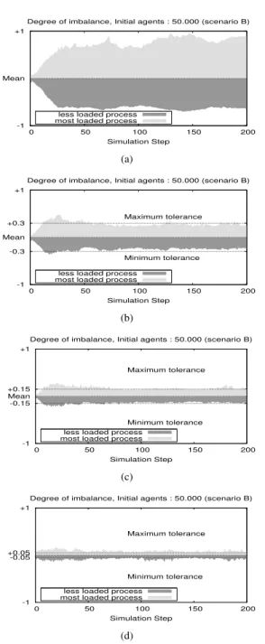
Fig. 8: Degree of computing imbalance varying the tolerance factor, for the scenario B on 128 processes.

Figure 8 shows the variability of the degree of imbalance for different values of tolerance factor. This Figure shows the degree of imbalance that decreases when the tolerance factor is increased, but the Load Balancing schema is triggered more frequently. Consequently, values of Table 5 expose that the overhead of our schema is greater when reducing the tolerance factor. For this reason, better results in terms of

execution time are related to finding a tolerance value which does not imply an excessive overhead for exchanging agents.

6. Conclusion

Due to the different rules of behavior and the high levels of interaction between agents, the ABMS applications may present computational and communicational imbalances during the simulation process. Therefore, to solve this prob-lem, the simulation environment should be equipped with migration mechanisms to move agents between overloaded and underloaded processes.

In this paper, we have presented a Dynamic Load Balanc-ing schema is proven in a model with high-level workload variability. For both scenarios, our schema obtains good results improving simulation execution time, and keeps a quite stable overhead. This overhead is caused by the amount of exchanges during the load balancing process. In addition, our modification of the FLAME framework for automatically generating agent migration functions. In this manner, the workload among the different processes can be adjusted dynamically during the simulation. In future work, we will aim our research on balancing communication times.

Acknowledgment

This work was funded by MICINN Spain, under the project TIN2011-28689-C02-01.

References

[1] R. K. Standish and R. Leow, “Ecolab: Agent based modeling for c++ programmers,”CoRR, vol. cs.MA/0401026, 2004.

[2] N. Collier and M. North, “Repast sc++: A platform for large-scale agent-based modeling,”Large-Scale Computing Techniques for Com-plex System Simulations, 2011.

[3] M. Kiran, P. Richmond, M. Holcombe, L. S. Chin, D. Worth, and C. Greenough, “Flame: simulating large populations of agents on parallel hardware architectures,” inAAMAS, 2010, pp. 1633–1636. [4] B. Zhou and S. Zhou, “Parallel simulation of group behaviors,” in

Proceedings of the 36th conference on Winter simulation, ser. WSC ’04. Winter Simulation Conference, 2004, pp. 364–370.

[5] G. Zheng, E. Meneses, A. Bhatele, and L. V. Kale, “Hierarchical load balancing for charm++ applications on large supercomputers,” inProceedings of the 2010 39th International Conference on Parallel Processing Workshops, ser. ICPPW ’10. Washington, DC, USA: IEEE Computer Society, 2010, pp. 436–444.

[6] D. Zhang, C. Jiang, and S. Li, “A fast adaptive load balancing method for parallel particle-based simulations,”Simulation Modelling Practice and Theory, vol. 17, no. 6, pp. 1032–1042, 2009.

[7] G. Vigueras, M. Lozano, and J. M. Orduña, “Workload balancing in distributed crowd simulations: the partitioning method,”J. Supercom-put., vol. 58, no. 2, pp. 261–269, Nov. 2011.

[8] B. Cosenza, G. Cordasco, R. De Chiara, and V. Scarano, “Distributed load balancing for parallel agent-based simulations,” in Proceedings of the 2011 19th International Euromicro Conference on Parallel, Distributed and Network-Based Processing, ser. PDP ’11. Washington, DC, USA: IEEE Computer Society, 2011, pp. 62–69.

[9] R. Solar, R. Suppi, and E. Luque, “Proximity load balancing for distributed cluster-based individual-oriented fish school simulations,”

Procedia Computer Science, vol. 9, no. 0, pp. 328 – 337, 2012, proceedings of the International Conference on Computational Science, ICCS 2012.