WORKING PAPER NO. 11-2
A DYNAMIC MODEL OF UNSECURED CREDIT
Daniel R. Sanches
Federal Reserve Bank of Philadelphia
A Dynamic Model of Unsecured Credit
Daniel R. Sanches
Federal Reserve Bank of Philadelphia
December 2010
I thank Steve Williamson, Gaetano Antinolfi, James Bullard, Rody Manuelli, Thorsten Koeppl,
Cyril Monnet, William Roberds, Pedro Gomis-Porqueras, Randy Wright, Costas Azariadis,
David Andolfatto, and Mitchell Berlin for helpful comments. I also thank participants at the 2nd
European Economic Review Talented Economists Clinic in Florence, the 2009 Summer
Workshop on Money and Banking at the Federal Reserve Bank of Chicago, and the Search and
Matching Workshop at the Federal Reserve Bank of Philadelphia. Finally, I would like to thank
seminar participants at the Federal Reserve Bank of Richmond, Federal Reserve Bank of
Philadelphia, University of Kansas, University of Toronto, Federal Reserve Board, Bank of
Canada, University of Miami, PUC-Rio, and FGV-EPGE.
Correspondence to Sanches at Research Department, Federal Reserve Bank of Philadelphia, Ten
Independence Mall, Philadelphia, PA 19106-1574; phone: (215) 574-4358; Fax: (215) 574-4303;
e-mail:
Daniel.Sanches@phil.frb.org
.
The views expressed in this paper are those of the author and do not necessarily reflect those of
the Federal Reserve Bank of Philadelphia or the Federal Reserve System. This paper is available
free of charge at www.philadelphiafed.org/research-and-data/publications/working-papers/
Abstract
We study the terms of credit in a competitive market in which sellers (lenders) are willing to repeatedly …nance the purchases of buyers (borrowers) by engaging in a credit relationship. The key frictions are: (i) the lender is unable to observe the borrower’s ability to repay a loan; (ii) the borrower cannot commit to any long-term contract; (iii) it is costly for the lender to contact a borrower and to walk away from a contract; and (iv) transactions within each credit relationship are not publicly observable. The lender’s optimal contract has two key properties: delayed settlement and debt forgive-ness. Asymmetric information gives rise to the property of delayed settlement, which is a contingency in which the lender allows the borrower to defer the repayment of his loan in exchange for more favorable terms of credit within the relationship. This property, together with the borrowers’lack of commitment, gives rise to debt forgiveness. When the borrower’s participation constraint binds, the lender needs to “forgive” part of the borrower’s debt to keep him in the relationship. Finally, we study the impact of the changes in the initial cost of lending on the terms of credit.
Keywords: Unsecured Loans; Dynamic Contracting; Delayed Settlement; Debt For-giveness; Initial Cost of Lending. JEL Classi…cation Numbers: D8, E4, G2.
1. INTRODUCTION
We study long-term credit arrangements in the Lagos-Wright model; see Lagos and Wright (2005) and Rocheteau and Wright (2005). To motivate trade and credit, we consider a ver-sion of the model in which there is an intertemporal double coincidence of wants. To allow for the use of intertemporal incentives, we depart from the baseline model by relaxing the assumption that agents cannot engage in enduring relationships. Speci…cally, we charac-terize the terms of credit in a competitive market in which sellers (lenders) are willing to repeatedly …nance the purchases of buyers (borrowers) by extending direct credit. Lenders enter the credit market by posting the terms of the contract, and each borrower chooses with whom he wants to engage in a credit relationship. We use the techniques of the dynamic contracting literature to solve for the lender’s optimal contract.1
Our approach is consistent with the endogenously incomplete markets literature [see Sleet (2008)] in which trading arrangements are derived from primitive frictions instead of assumed. The frictions we choose to model are as follows. First, lenders are unable to observe a borrower’s ability to repay a loan. Second, lenders can commit to some contracts, whereas borrowers cannot commit to any contract. Speci…cally, lenders are committed to delivering any long-term contract that does not result in an expected value that, at any moment, is lower than that associated with autarky, whereas borrowers are unable to commit to any long-term contract. Third, transactions within each credit relationship are not publicly observable, which captures the idea that information is dispersed in credit markets. Fourth, it is costly for a lender to contact a borrower, as in Drozd and Nosal (2008) and Livshits, MacGee, and Tertilt (2009), and it is also costly for a lender to walk away from a contract with a borrower, as in Phelan (1995). Given these frictions, we derive the terms of the contract that lenders o¤er to borrowers in a competitive credit market.
We build on the analysis in Phelan (1995) in which a lender and a borrower engage in a dynamic credit relationship. In Phelan’s analysis, the borrower is able to quit from the
1
See Green (1987); Thomas and Worrall (1990); Atkeson and Lucas (1992, 1995); Kocherlakota (1996); Aiyagari and Williamson (1999); and Krueger and Uhlig (2006).
lender’s contract only at the beginning of each periodbefore learning his income realization. Thus, there is a one-period commitment to a contract. The Lagos-Wright structure of sequential trade and intertemporal double coincidence of wants makes the timing within each period critical. There is a distinct settlement stage following each round of transactions, which allows the borrowers to periodically discharge their past debts.2 However, there is a friction that a¤ects a borrower’s ability to repay his past obligations during the settlement stage, which creates a motive for long-term credit arrangements. Speci…cally, the Lagos-Wright model results in a sequence ofex post participation constraints for the borrower (as opposed to oneex anteconstraint as in Phelan’s analysis) because the latter has an incentive to walk away precisely at the settlement stage. As a result, we obtain a model of unsecured lending that allows us to characterize the loan schedule that the lender is committed to delivering as well as the repayment amounts that are required from the borrower.
One important characteristic of a credit transaction is that settlement takes place at a future date: each credit transaction between a borrower and a lender necessarily creates a liability for the borrower that needs to be settled some time in the future. Because the ‡ow of payments between them is explicit in the Lagos-Wright framework, we can use the model to make predictions with respect to movements in loan and repayment amounts over time, which are observable characteristics in credit markets. Another advantage of the model is that, because of the existence of an intertemporal double coincidence of wants, the gains from trade within a credit relationship are also explicit: There is a surplus from a match between a borrower and a lender that needs to be shared. Long-term unsecured credit is the optimal …nancial arrangement for the lender given that she needs to post the terms of the contract in order to enter the credit market. Moreover, the intertemporal punishments and rewards implicit in the lender’s optimal contract are meaningful in terms of observed behavior in credit markets. As a result, we can use the model to study revolving lines of credit and debt renegotiation as equilibrium outcomes.
2
Koeppl, Monnet, and Temzelides (2008) use the Lagos-Wright framework to show that the existence of a settlement round in which the agents have an opportunity to discharge their debt is essential for implementing constrained e¢ cient allocations.
The focus on the borrower’s lack of commitment is crucial for the analysis. To con-struct a model of bilateral contracting, one crucial step consists of identifying for whom the commitment problem is more relevant. For modeling an insurance contract, the relevant commitment problem is for the insurer (the principal), who has received the premium pay-ments from the policyholders and has capitalized to make a disbursement when a speci…c event materializes. For modeling a credit contract, the relevant commitment problem is for the borrower (the agent), who has received a loan and is required to settle his debt at some speci…ed date. In our model, the party who lacks commitment can certainly be identi…ed as a borrower, which makes the analysis special for studying unsecured lending. For this reason, the role of the ex post participation constraints is crucial for the interpretation of the optimal dynamic contract as a long-term credit arrangement.
We characterize the lender’s optimal contract and derive two key properties: delayed settlement and debt forgiveness. The property of delayed settlement is a contingency that allows the borrower to defer the repayment of his loan to a future date. As a result of the optimal provision of intertemporal incentives, the lender allows the borrower to delay his repayment in exchange for more favorable terms of credit for future transactions within the credit relationship, which translate into decreasing loan amounts and weakly increasing repayment amounts. This mechanism arises because the lender needs to provide incentives for collecting a repayment from the borrower.
The second key property of the lender’s optimal contract is debt forgiveness. As we have seen, a delayed repayment worsens the terms for the borrower. If the borrower postpones his repayment for long enough (due to a string of unfavorable shocks to his ability to repay), his participation constraint will eventually bind because the lender will keep worsening the terms of the contract, which in turn creates an incentive for him to walk away from his current contract and sign with another lender. To keep him in the relationship, the lender with whom he is currently paired needs to “forgive” part of his previous debt. As a result, there is a minimum loan amount that the lender is committed to delivering to the borrower and a maximum repayment amount that she is able to collect from him because of competition in the credit market and a lack of commitment by borrowers. Thus, it is
the combination of asymmetric information with lack of commitment that results in debt forgiveness as an equilibrium outcome.
Finally, we use the model to study the e¤ects of a change in the initial cost of lending on the terms of the contract.3 A lower cost of starting a credit relationship has the following impact on the equilibrium outcome: (i) each borrower is better o¤ from the perspective of the contracting date; (ii) a borrower’s expected discounted utility ‡uctuates within a smaller set; and (iii) each lender is uniformly worse o¤ex post. A lower cost of entry in the credit market leads to more competition among lenders, which in turn results in more favorable terms of credit for each borrower.
2. THE MODEL
Time is discrete and continues forever, and each period is divided into two subperiods. There are two types of agents, referred to as borrowers and lenders. In the …rst subperiod, a lender is able to produce the unique perishable consumption good but does not want to consume, and a borrower wants to consume but cannot produce. In the second subperiod, we have the opposite situation: A borrower is able to produce but does not want to consume, and a lender wants to consume but cannot produce. Production and consumption take place within each subperiod. This generates an intertemporal double coincidence of wants, and for this reason, we refer to the …rst subperiod as the transaction stage and to the second subperiod as the settlement stage. The types (borrower and lender) refer to the agent’s role in the transaction stage. The production technology allows each agent to produce one unit of the good with one unit of labor. Each agent receives an endowment of h > 0 units of time in each subperiod. Let 2(0;1)be the common discount factor over periods.
The lender’s utility in period t is given by (1 ) qtl+xlt , where qtl is production
3
We think this is an interesting exercise because there is signi…cant evidence showing that the cost of starting a credit relationship has fallen signi…cantly over the past two decades. For instance, Mester (1997) points out that the use of credit scoring has signi…cantly reduced the time and cost of the loan approval process. Barron and Staten (2003) and Berger (2003) also provide evidence suggesting that advances in information technology have reduced the cost of processing information for lenders.
of the good in the transaction stage and xlt is consumption of the good in the settlement stage. The borrower’s momentary utility of consuming qtb units of the consumption good in the transaction stage is given by(1 )u qtb . Assume that u :R+ ! R is increasing, strictly concave, and continuously di¤erentiable. Let H denote the inverse of u, and let
wa u(0)denote the value associated with autarky. Producingytb units of the good in the settlement stage generates disutility (1 )ytb for a borrower. However, there is a friction that a¤ects a borrower’s ability to produce goods in the settlement stage. With probability a borrower is unable to produce the consumption good, and with probability 1 a borrower can produce the good using the linear production technology. This productivity shock is independently and identically distributed over time and across borrowers. Each borrower learns his productivity shock at the beginning of the settlement stage, which is privately observed. Finally, let D denote the set of expected discounted utilities for the borrower.
Suppose that there is a large number of borrowers and lenders, with the set of lenders su¢ ciently large.4 There is a one-shot cost k > 0 in terms of the consumption good for a lender to post a credit contract to enter the credit market, which speci…es consumption and production by each party as a function of the available information. As in Drozd and Nosal (2008) and Livshits, MacGee, and Tertilt (2009), we motivate this assumption as the cost of contacting a borrower in the credit market and starting a credit relationship. We assume that each lender can have at most one borrower; it is in…nitely costly for a lender to contact two borrowers at the same time. Given that the lenders are risk-neutral, this assumption is innocuous in that it does not a¤ect the terms of the contract that they o¤er in the credit market, allowing us to focus on the bilateral gains from trade associated with a credit relationship. Each lender also has to pay a cost >0 to walk away from her current contract. As in Phelan (1995), we motivate this assumption as a legal cost that a lender has to pay to e¤ectively walk away from her current contract with a borrower.
Only the agents in a bilateral meeting observe the history of trades. Other agents in the economy observe a break in a particular match but do not observe the history of trades
4
in that match. Notice that there are gains from trade since a lender can produce the consumption good for a borrower in the …rst subperiod (transaction stage) and a borrower can produce the good for a lender in the second subperiod (settlement stage). An important feature of the model is that, with probability , a borrower is unable to produce the good in the second subperiod and settle his debt.
3. EQUILIBRIUM
In this section, we characterize the stationary equilibrium allocation under a particular pricing mechanism: price posting by lenders. To enter the credit market, a lender needs to post a contract to attract a borrower and start a credit relationship. Although it is costly for a lender to make contact with a borrower, there is free entry of lenders in the credit market. We characterize the terms of the contract in each credit relationship in the economy and restrict attention to a symmetric, stationary equilibrium in which each borrower receives a market-determined credit contract o¤ered by a lender that promises him expected discounted utility w , from the perspective of the contracting date. Each lender needs to provide incentives to induce the desired behavior by a borrower given that a borrower’s ability to repay a loan is unobservable.5
We assume that lenders can commit to some credit contracts, whereas borrowers cannot commit to any contract. Speci…cally, each lender is committed to delivering any long-term contract that does not result in an expected discounted utility that, at any moment, is lower than that associated with autarky; recall that a lender always has the option of remaining inactive. On the other hand, borrowers cannot commit to any long-term contract and can walk away from a credit relationship at any moment without any pecuniary punishment. As we will see, a lender’s optimal contract results in a long-term relationship from which neither party wants to deviate.
The expected discounted utility w 2 D associated with the market contract must be
5Throughout the paper, we restrict attention to Markovian equilibrium in that borrowers are not
di¤er-entiated by whether they have ever walked away from a contract and the market expected utility isw at each date.
such that it makes each lender indi¤erent between entering the credit market by posting a contract and remaining inactive, from the perspective of the contracting date. As a result, some lenders post a contract and successfully match with a borrower, while others do not post a contract and remain inactive. When o¤ering her own contract, each lender takes as given the contracts o¤ered by the other lenders. The only relevant characteristic about these contracts is the expected discounted utility w that each borrower associates with them. This is the utility that a borrower obtains by accepting a lender’s contract, from the perspective of the signing date. The equilibrium is symmetric because every active lender o¤ers the same credit contract.
The market contract mustalways result in an expected discounted utility for a borrower that is greater than or equal tow . If the market contract promises, in a given period, an expected discounted utility w0 for a borrower that is less thanw , the latter can do better by reneging on his current contract and starting a new credit relationship with another lender. Recall that inactive lenders observe the dissolution of a credit relationship and may be willing to enter the credit market. Given that there is free entry of lenders and limited commitment, we can have an equilibrium only if the lowest promised expected discounted utility at any moment is exactly w .
3.1. Recursive Formulation of the Contracting Problem
A contract speci…es in every period a transfer of the good from the lender to the borrower in the transaction stage and a repayment (a transfer of the good from the borrower to the lender) in the settlement stage as a function of the available history of reports by the borrower. These are reports about a borrower’s ability to produce goods in the settlement stage. Let t 1 = 0; 1; :::; t 1 2 f0;1gtdenote a partial history of reports, where = 0
means that a borrower is unable to produce the good in the settlement stage at date and
= 1 means that he is able to produce it in the settlement stage at date .
In equilibrium, each active lender chooses to o¤er a long-term contract, which means that she matches with a borrower at the …rst date and keeps him in the credit relationship
forever. The long-term contract speci…es quantities produced and transferred within each subperiod. We say that in each period t there is a transaction between a borrower and a lender that consists of a loan amount from the lender to the borrower in the …rst subperiod (transaction stage) and a repayment amount in the second subperiod (settlement stage) that is contingent on the report of the productive state of nature ( t= 1).
The optimal contracting problem has a recursive formulation in which we can use a borrower’s expected discounted utility w2 D as the state variable. The optimal contract minimizes the expected discounted cost for the lender of providing expected discounted utility w to the borrower subject to incentive compatibility. As we have seen, w is the lower bound on the set of expected discounted utilities. Let w denote the upper bound, which is endogenously determined but is taken as given for now. LetC(w ;w): [w ; w]!R
denote the expected discounted cost for the lender, which satis…es the following functional equation: C(w ;w)(w) = min '2 (w ;w)(w) 8 < : (1 ) [H(u) (1 )y1] + C(w ;w)(w0) + (1 )C(w ;w)(w1) 9 = ;. (1)
Here, the choices are given by'= (u; y1; w0; w1), whereudenotes a borrower’s momentary
utility of consumption in the transaction stage, y1 denotes his production in the settlement
stage given that he is able to produce the good, and w denotes his promised expected discounted utility at the beginning of the following period given that his report in the current period is 2 f0;1g. Recall that = 0 means that a borrower is unable to produce the good in the settlement stage and that = 1 means that he is able to produce it. The constraint set (w ;w)(w)consists of all 'inD [0; h] [w ; w]2 satisfying the borrower’s participation constraints,
w0 w , (2)
(1 )y1+ w1 w , (3)
the borrower’s truth-telling constraint,
and the promise-keeping constraint,
(1 ) [u (1 )y1] + [ w0+ (1 )w1] =w. (5)
It can be shown that, for any …xed lower bound w and upper bound w, there exists a unique continuously di¤erentiable, strictly increasing, and strictly convex functionC(w ;w):
[w ; w]!Rsatisfying the functional equation (1). Letu^: [w ; w]!D,y: [w ; w]![0; h], and g : [w ; w] f0;1g ! [w ; w] denote the associated policy functions, which can be shown to be uniquely determined, continuous, and bounded.
Given our choice of working on the space of expected discounted utilities,wnow summa-rizes the borrower’s partial history of reports. As we have mentioned, we say that there is a transaction between a lender and a borrower in the current period whose terms are given by fH[^u(w)]; y(w)g. The quantity H[^u(w)] gives the loan amount from the lender to the borrower in the transaction stage, and the quantity y(w) gives the repayment amount in the settlement stage contingent on the report of the productive state of nature. Both quantities depend on w, which means that the terms of credit change over time according to the history of transactions.
Although the lender is committed to delivering a long-term contract, she cannot commit to a contract that gives her an expected discounted utility that, at any moment, is lower than that associated with autarky. As a result, individual rationality for the lender requires
that C(w ;w)(w) holds for all w 2 [w ; w]. Recall that a lender needs to pay a cost
> 0 in order to break up a credit relationship. As in Phelan (1995), we motivate this assumption as a legal cost that a lender has to pay to e¤ectively walk away from her current contract with a borrower.
Next we show that, for some values for the lower bound w , there exists an upper bound
w = w(w ; ) on the set of expected discounted utilities that gives the highest promised expected utility to which a lender can commit given that the lowest expected utility that can be promised isw . As we will see later, the market utilityw is determined endogenously and is such that it makes each lender indi¤erent between entering the credit market by posting a contract and remaining inactive. Before we proceed, it is useful to de…ne the following set:
for any given value for >0, letI( ) = w:w wa and C(w;w)(w) . Notice that for any w wa we haveC(w;w)(w) =H(w) 0. This is the lender’s expected discounted cost
of delivering expected discounted utilitywto a borrower given that the lender is constrained to choosing the same continuation values regardless of the state reported by the borrower. In this case, it is not possible to obtain a repayment from the borrower: The only incentive-feasible value for y1 is zero. Because H(w) is strictly increasing, we have that I( ) is an
interval that shrinks as !0.
Lemma 1 For anyw 2I( ), there exists an upper bound w(w ; ) on the set of expected
discounted utilities such that C(w ;w(w ; ))[w(w ; )] = .
Proof. Let wF( ) denote the expected discounted utility for a borrower such that the
expected discounted cost for a lender of providingwF ( )given complete information equals
. De…ne the function : [w ; wF( )] ! [w ; wF ( )] as follows. For any given w 2
[w ; wF( )], if there is no w0 2 [w ; w] such that C(w ;w)(w0) = , then (w) = w .
Otherwise, (w) equals the highest point w0 in[w ; w] for which C(w ;w)(w0) = . Notice
that C(w ;w )(w ) by assumption, which implies that (w ) = w . For any other w
such that (w) =w, it must be that C(w ;w)(w) = .
Construct a sequence wk 1
k=0 of candidates for the upper bound w in the following
way. Let w0 = wF( ). We have that C(w ;w0) w0 , with strict inequality if the
truth-telling constraint (4) binds. Also, notice that (w ;w )(w ) (w ;w0)(w ), which
implies that C(w ;w0)(w ) C(w ;w )(w ) . Continuity implies that there exists w1 2 w ; w0 such that C(w ;w0) w1 = . This means that w1 = w0 w0. We proceed
in the same fashion to de…ne w2. From the fact that C(w ;w0) C(w ;w1), it follows that
C(w ;w1) w1 C(w ;w0) w1 = . Given that (w ;w )(w ) (w ;w1)(w ), we have that
C(w ;w1)(w ) C(w ;w )(w ) . Again, continuity implies that there existsw2 2 w ; w1
such thatC(w ;w1) w2 = . This means thatw2= w1 w1. Notice then that wk 1
k=0
is a nonincreasing sequence on a closed interval. As a result, it converges to a pointw1in the interval[w ; wF( )]. The Theorem of the Maximum guarantees that (w) C(w ;w)(w)
To ease notation, de…neCw (w) C(w ;w(w ; ))(w)and de…ne the setDw [w ; w(w ; )].
Given thatCw (w)is strictly increasing inw, it follows thatCw (w) for allwin the set
Dw . This means that, for any given lower boundw ,Dw gives the set of promised expected
discounted utilities that are actually incentive-feasible. If the truth-telling constraint binds, then it follows that w(w ; ) > w for any lower bound w satisfying C(w ;w )(w ) . Next we show that the truth-telling constraint indeed binds for any w in Dw . But …rst
notice that the truth-telling constraint (4), together with the constraint 0 y(w) h, implies that g(w;1) g(w;0) for all w 2 Dw , which means that the optimal contract
needs to assign a higher promised expected discounted utility to a borrower contingent on the realization of the productive state of nature to e¤ectively induce truthful reporting.
Lemma 2 The truth-telling constraint (4) binds for any w2Dw .
Proof. Suppose that
(1 )y1+ w1 > w0 (6)
holds at the optimum. This implies that
(1 )y1+ w1 > w (7)
must also hold at the optimum. Now, reduce the left-hand side of (6) and (7) by a small amount > 0 so that both inequalities continue to hold. De…ne w0
1 = w1 and
w00=w0+(1 ) . Notice that w00+(1 )w10 = w0+(1 )w1andw10 w00< w1 w0.
The strict convexity of Cw implies that
Cw w00 + (1 )Cw w10 < Cw (w0) + (1 )Cw (w1),
so that the value of the objective function on the right-hand side of (1) falls. Since all constraints continue to be satis…ed, this implies a contradiction. Q.E.D.
An immediate consequence of the previous result is that w < w(w ; ) for any given
3.2. Existence and Uniqueness of Stationary Equilibrium
Now, we need to ensure that there exists a market-determined expected discounted utility
w associated with a market contract that makes each lender indi¤erent between posting a contract and remaining inactive. This is equivalent to showing the existence of an equilib-rium.
Formally, a stationary and symmetric equilibrium consists of a cost function Cw:Dw ! R; policy functionsu^:Dw !D,y:Dw![0; h],g:Dw f0;1g !Dw; and a market utility
w such that: (i) Cw satis…es (1);(ii) (^u; y; g)are the optimal policy functions associated
with (1); and(iii) w satis…es the free-entry condition:
Cw (w ) + (1 )k= 0. (8)
The market utility w gives the expected discounted utility for a borrower at the signing date. Due to limited commitment and free entry of lenders in the credit market, it is also the lower bound on the set of expected discounted utilities.
Proposition 3 Given > 0, there exist k
¯( ) and k( ), with 0 ¯k( ) < k( ), such that there exists a unique expected discounted utility w satisfying (8) provided that k 2
k
¯ ( ); k( ) .
Proof. Notice thatCwa(wa)<0. We needk >0 to be such thatCwa(wa) + (1 )k <0 andCw (w ) + (1 )k 0, wherew = supI( ). IfCw (w ) 0, then the lower bound
k
¯( ) equals 0 and the upper bound k( ) is given by the value ofk satisfying Cwa(w
a) +
(1 )k = 0. If Cw (w ) < 0, then the lower bound k
¯( ) is given by the value of k satisfying Cw (w ) + (1 )k = 0 and the upper bound k( ) is given by the value of k
satisfying Cwa(wa) + (1 )k = 0. Given that ^ (w) Cw(w) is continuous in w, there existsw 2[wa; w ]such that ^ (w ) + (1 )k= 0 provided that k2 k
¯( ); k( ) . To show uniqueness, de…ne the mapping : [wa; w ] ! [wa; w ] as follows. If Cw +
(1 )kis always greater than zero on [w; w ], then (w) =wa. Otherwise, (w) equals
in w. To verify this claim, we …rst need to show that w(w; ) is nonincreasing in w. Fix a lower bound w0 in the set [wa; w ], and consider the associated upper bound w(w0; ). Take another point w00 > w0 in the set [wa; w ]. Notice that C(w0;w(w0; )) C(w00;w(w0; )). Thus, we have that C(w00;w(w0; ))[w(w0; )] given that C(w0;w(w0; ))[w(w0; )] = by
the de…nition of w(w0; ). This implies that w(w00; ) w(w0; ), and we conclude that
w(w; ) is indeed nonincreasing in w. The fact that w(w; ) is nonincreasing then implies that raising the lower bound w only tightens the constraint set. As a result, the point at which Cw+ (1 )k equals zero is a nonincreasing function of the lower bound w, which
means that can have at most one …xed point. Q.E.D.
Notice thatex anteeach lender gets zero expected discounted utility by posting a contract.
Ex post a lender gets a higher utility, given thatCw (w )<0. Moreover, as the contract is
executed, there is no history of reports by the borrower that gives the lender an expected discounted utility that is lower than that associated with autarky. For this reason, neither the lender nor the borrower …nds it optimal to renege on the credit contract.
If is su¢ ciently small, then it is possible to have k
¯( )>0. This means that a stationary equilibrium may not exist if the initial cost of lending k is too small (below k
¯( )). To verify this claim, we …rst need to show that w(w; ) is nondecreasing in . Notice that
wF( 0) < wF( ) for any 0 < 0 < . Also, notice that I( 0) I( ). If we …x w2I( 0)
and construct the candidate sequences for the upper bound on the set of expected discounted utilities in the same way as in the proof of Lemma 1, we will …nd that w(w; 0) w(w; ),
which means thatw(w; )is indeed nondecreasing in . It is straightforward to show that we must have Cwa(wa) <0 for any given >0. This means that, for a su¢ ciently small value for , we have Cw (w ) < 0. We prove this claim in the appendix. In the proof of
Proposition 3, we need to have k such that Cw (w ) + (1 )k 0. If Cw (w ) <0, it
could be necessary to havek >0, which gives rise to a strictly positive lower bound k ¯( ). It is important to keep in mind the possibility that a stationary equilibrium may not exist when both the cost of walking away from a credit contract and the initial cost of lending
of changing the initial cost of lending k holding …xed. However, there may not exist a stationary equilibrium if we reduce the initial cost of lending too much when is arbitrarily small. In Phelan (1995), we have k= 0 and >0. Even though the incentive constraints in his analysis are di¤erent from ours, the same issue of nonexistence applies: We cannot guarantee thatCw (w ) 0holds for arbitrarily small values for the cost , in which case
we cannot guarantee the existence of equilibrium.
3.3. Properties of the Optimal Contract
In this subsection, we characterize the policy functionsu^(w),y(w), and g(w; ), and es-tablish some important properties of the optimal contract. We can rewrite the optimization problem on the right-hand side of (1) in the following way. The relevant constraints for the optimization problem are (2),
(1 )y1+ w1 = w0, (9)
and
(1 ) (u y1) + w1=w. (10)
Here, (9) is (3) with equality, and (10) is obtained by combining (3) and (5). Substituting (9) and (10) into (1), the problem now consists of choosingy1 andw1 to minimize:
(1 ) H w w1 1 +y1 (1 )y1 + 8 < : Cw h w1 (1 )y1 i + (1 )Cw (w1) 9 = ;, subject to w w1 w(w ; ),0 y1 h, and w1 (1 ) y1 w . (11)
The …rst-order conditions for the optimal choice of y1 are
H0 w g(w;1) 1 +y(w) C 0 w [g(w;0)] + (w) 1 , (12) ify(w)< h, and H0 w g(w;1) 1 +y(w) C 0 w [g(w;0)] + (w) 1 , (13)
ify(w)>0. The …rst-order condition for the optimal choice ofw1 is H0 w g(w;1) 1 +y(w) 8 < : Cw0 [g(w;0)] + (1 )Cw0 [g(w;1)] (w) 9 = ;, (14)
with equality if g(w;1)< w(w ; ). Also, we have that
(w) g(w;1) (1 )y(w) w = 0, (15)
where (w) 0 is the Lagrange multiplier associated with constraint (11). Finally, the envelope condition is given by
Cw0 (w) =H0 w g(w;1)
1 +y(w) , (16)
for any value of win the interior of the set Dw .
Now, we establish some properties of the repayment schedule y(w) and of the optimal continuation value g(w; ), with 2 f0;1g. The latter gives the borrower’s expected dis-counted utility at the beginning of the following period associated with the market contract as a function of his initially promised expected discounted utility w and his report in the settlement stage at the current date. If the borrower’s expected discounted utility falls in the subsequent period relative to the current period, this means that the terms of the contract become less favorable for him –and, as a result, more favorable for the lender with whom he is paired.
Proposition 4 g(w;1) w for allw in the interior of Dw .
Proof. Suppose that g(w;1)< wfor some w in the interior ofDw . Given thatg(w;1)<
w < w(w ; ), (14)-(16) imply
Cw0 (w) = Cw0 [g(w;0)] + (1 )Cw0 [g(w;1)] (w).
Recall thatg(w;1) g(w;0)and thatCw (w)is strictly convex inw. As a result, we have
where the last inequality follows because (w) 0. But this results in a contradiction. Hence, we conclude thatg(w;1) w for all win the interior of Dw . Q.E.D.
A repayment by the borrower in the settlement stage results in at least the same terms of credit for future transactions within the credit relationship. If the borrower reports the productive state of nature in the settlement stage and, as a result, makes a repayment
y(w) to his lender, his expected discounted utility at the beginning of the following period
g(w;1)either rises or remains the same. This means that the terms of credit for all future transactions within the relationship either become more favorable or remain the same for him. This property of the optimal contract arises because the lender cannot observe the borrower’s ability to repay a loan in the settlement stage. As a result, the lender needs to induce a repayment from a borrower who is currently productive in the settlement stage by promising him at least the same terms of credit for future transactions as those promised for the current transaction.
Proposition 5 y(w) is nonincreasing on Dw .
Proof. Suppose that there is an interval D~ Dw on which y(w) is increasing. Then,
there is an interval D^ D~ on which 0 < y(w) < h. Notice that (12)-(14), together with (16), imply thatg(w;1) is constant on D^. Then, (9) implies thatg(w;0)is decreasing on
^
D, which in turn implies that (w) = 0 for all w2D^. From (16), we must have
Cw0 (w) = Cw0 [g(w;0)] + 1
for all w 2 D^. But this implies a contradiction. Therefore, it must be that y(w) is nonincreasing on Dw as claimed. Q.E.D.
Proposition 6 The function g(w;0) has the following properties: (i) g(w;0)< w for all w > w and (ii) g(w ;0) =w .
Proof. First, notice that we must havey(w)>0for allwin the interior ofDw . To verify
this claim, suppose that y(w) = 0 for some w 2 (w ; w(w ; )). Because y(w) is nonin-creasing, we must have y(w0) = 0for all w0 2[w ; w(w ; )]. Notice that g[w(w ; );0] =
g[w(w ; );1] = w(w ; ) because y[w(w ; )] = 0 and u^[w(w ; )] = w(w ; ). Then, (14)-(16) imply thatCw0 (w) Cw0 [w(w ; )], which results in a contradiction. Therefore, we must have y(w)>0for all w2(w ; w(w ; )). As a result, g(w;1)> g(w;0)for all w
in the interior of Dw .
Suppose that g(w;0) w for somew > w . From (14)-(16), we have that
Cw0 (w) Cw0 [g(w;0)] + (1 )Cw0 [g(w;1)]> Cw0 (w),
where the last inequality follows from the fact that Cw (w) is strictly convex in w and
the fact that g(w;1) > g(w;0). But we obtain a contradiction. Hence, we must have
g(w;0)< w for allw > w . Sinceg(w;0)is continuous in w, it follows thatg(w ;0) =w . Q.E.D.
If the borrower defers his repayment to the lender in the settlement stage, then the terms of the contract become less favorable for him within the credit relationship. As a result of intertemporal allocation of resources by a risk-neutral lender, a delayed repayment is compensated by more favorable terms of credit for the lender in future transactions. When the borrower reports the unproductive state and, as a result, postpones his repayment to the lender, such an action creates a liability for the borrower, which alters the terms of credit for the subsequent transaction within the relationship. Hence, the property of delayed settlement is part of an optimal mechanism through which the lender obtains more favorable terms for future transactions within the relationship.
Proposition 7 There exists >0 such that g(w;0) =w for allw2[w ; w + ).
Proof. Suppose that g(w +";0)> w for all" >0. Then, (14)-(16) require that
Cw0 (w +") Cw0 [g(w +";0)] + (1 )Cw0 [g(w +";1)]
holds for all " > 0, which in turn requires that lim"!0g(w +";1) = w . But, from (9),
y(w )>0 impliesg(w ;1)> w , which results in a contradiction. Q.E.D.
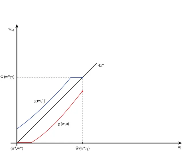
Not only the borrower’s participation constraint (2) binds at w , but it also binds for values ofwin a neighborhood ofw . This means that a borrower’s participation constraint
not only binds at the signing date, but it also binds after a …nite sequence of adverse productivity shocks. In the following section, we exploit the economic implications of the previous result. In Figure 1, we depict the schedulesg(w;0)and g(w;1).
Notice that, becausey(w)>0for allwin the interior of Dw and y(w)is nonincreasing
on Dw , we must havey(w ) >0, which gives the maximum repayment amount that the
lender can collect from the borrower within the credit relationship. Such an upper bound on the repayment amounts arises due to competition in the market for unsecured loans and a lack of commitment by borrowers. To clarify this point, consider a situation in which the borrower has experienced the unproductive state for several periods. Then, the lender …nds it optimal to worsen the terms of the contract for the borrower, resulting in a decreasing path for the borrower’s expected discounted utility w. As we have seen, his participation constraint will eventually bind, in which case the lender is unable to worsen the terms for the borrower because the latter has the option of walking away and signing with someone else. Thus, the borrower’s ability to quit from his current contract imposes an endogenous upper bound on the repayment amounts that can be collected from him (contingent on the realization of the productive state) as well as an endogenous lower bound on the loan amounts to which he is entitled.
Now we want to better characterize the loan amountsH[^u(w)]. Notice that the envelope condition (16) implies that the loan amount to which a borrower is entitled in the transaction stage is strictly increasing in his promised expected discounted utility w. As we have seen, the optimal provision of incentives by the lender results in a lower promised expected discounted utility for a borrower who reports the unproductive state and, as a result, fails to make a repayment. Thus, the loan amount that the borrower receives from the lender in the subsequent transaction stage shrinks, given that H[^u(w)] is an increasing function. This shows how the loan amount that the borrower receives from the lender in the current transaction depends on the history of trades within the credit relationship. Notice that
H[^u(w )]>0 gives the minimum loan amount to which a borrower is entitled during the transaction stage.
relationship. Notice that the expected return to the lender on the current transaction is given by
R(w) (1 )y(w)
H[^u(w)] , (17)
which summarizes the terms of credit for the current transaction as a function of w. Since the borrower’s expected discounted utilitywevolves over time within the setDw according
to the history of transactions between the borrower and the lender, we expect R(w) to ‡uctuate over time as a result. The following result is an immediate corollary from the fact thaty(w) is nonincreasing and that H[^u(w)] is increasing.
Proposition 8 The statistic R(w) de…ned by (17) is decreasing in w.
The statistic R(w), which is depicted in Figure 2, captures the evolution of the terms of credit according to the history of transactions (summarized byw). This means that R(w )
gives the worst terms of credit for the borrower, whereasR[w(w ; )]gives the best terms. The worse terms of credit for the borrower mean that he is entitled to a smaller loan amount in the transaction stage and/or is required to make a bigger repayment in the settlement stage, contingent on the realization of the productive state. Notice that the dynamics for R(w) depend critically on the assumption that the borrower’s productivity shock is privately observed. It is precisely because the lender is unable to verify the borrower’s ability to repay his loan that we observe the spreading of the borrower’s expected discounted utility. To make this point clear, we discuss the case with limited commitment and complete information in the appendix.
5. DEBT FORGIVENESS AND DELAYED SETTLEMENT
Suppose that at date t > 0 the borrower’s expected discounted utility is wt > w and
that he reports t = 0 in the settlement stage. The terms of the contract then become less favorable for him, which results in a lower promised expected discounted utility at date
on the borrower for delayed repayment at date t depends on the borrower’s repayment history, which is summarized by wt. In any case, following a delayed repayment, a smaller
loan amount is granted in the transaction stage at date t+ 1 and at least the same state-contingent repayment amount is required at datet+1(possibly a bigger repayment amount). Suppose thatg(wt;0)> w , which means that the borrower’s participation constraint (2)
is not binding at datet. If t+1 = 0, thenwt+2 =g(wt+1;0)< g(wt;0)so that the lender
keeps reducing the loan amount and requiring at least the same state-contingent repayment. Suppose now that g(wt;0) = w , in which case the borrower’s participation constraint
(2) binds at date t. In this case, the lender o¤ers the terms fH[^u(w )]; y(w )g for the transaction at date t+ 1. If t+1 = 0, then the lender continues to o¤er the same terms at date t+ 2. Why doesn’t the lender ask for a bigger repayment to compensate for the delayed repayment? As we have seen, H[^u(w )] is the endogenous lower bound on loan amounts and y(w ) is the endogenous upper bound on repayment amounts, which arise due to competition among lenders and a lack of commitment by borrowers. From the lender’s point of view, the terms fH[^u(w )]; y(w )g result in the highest expected return that she can get within a credit relationship, which is given by R(w ). The lender would like to require a bigger repayment amount from the borrower to compensate for the deferred repayments at dates tand t+ 1, but the maximum repayment amount that she can get is
y(w ).6
For any partial history of adverse shocks for the borrower that does not drive him tow , the optimal contract speci…es a nondecreasing (possibly increasing) repayment amount to compensate for deferred settlement. When the lower boundw is reached, that is, when the borrower’s participation constraint (2) eventually binds, the lender needs to “forgive” part of the borrower’s debt to prevent him from walking away. Thus, it is the combination of asymmetric information with borrowers’lack of commitment that results in debt forgiveness. If the borrowers were able to fully commit to the contract at datet= 0, then there would
6
Recall that the lender does provide incentives for truthful reporting and is willing to o¤er the terms
fH[^u(w )]; y(w )gfor the transaction at datet+ 1because the expected discounted value of her contract is strictly positive.
be no debt forgiveness: The lender would always be able to worsen the terms of the contract for the borrower whenever the latter deferred his repayment. To make this point clear, we characterize the optimal contract under full commitment and asymmetric information in the appendix.7
We interpret the states in which the borrower makes a repayment to the lender as the settlement of all current liabilities; that is, a repayment discharges all past debts. At the signing date t = 0, the borrower who is able to repay his loan is rewarded with more favorable terms of credit after discharging his debt. If he continues to repay his loans, he will be rewarded with at least the same terms of credit as those he previously had. If he reports the unproductive state at some date t, then he will delay the repayment of the loan that he received at datet. If the repayment eventually happens before he reaches the lower bound w (in which case his participation constraint will not bind), then settlement happens without debt forgiveness. Otherwise, settlement happens after part of his debt has been forgiven.
At date t= 0 or at any other datet for whichwt=w , the lender makes the minimum
loanH[^u(w )]to the borrower in the transaction stage. In the settlement stage, sheexpects
to receive the repayment amount y(w ), which is the largest incentive-feasible repayment amount. If the borrower reports t= 0, then the optimal contract speci…es that no repay-ment is required. Otherwise, the borrower produces and transfers the amounty(w ) to the lender. Following the partial history t= 0, the lender continues to o¤er the same terms of credit at date t+ 1. When the lender writes the optimal contract at date t= 0, she takes into account the possibility of receiving the repayment y(w ) many periods ahead, even though she is committed to making the minimum loan amountH[^u(w )]. In this instance, the lender forgives part of the borrower’s debt so that we can still interpret any repayment
7
This property of the optimal contract is related to the property of “amnesia” in Kocherlakota (1996), where a model of two-sided lack of commitment is analyzed; see also Ligon, Thomas, and Worrall (2002). In these models, the agents’endowments are publicly observable, and as a result, there is no need for inducing truthful reporting. Thus, the spreading of expected discounted utilities is not necessarily a property of the optimal contract, which is a critical aspect of our analysis.
as the discharge of all current liabilities (given that part of the debt is forgiven). Whenever the borrower reports t = 1 in the settlement stage and, as a result, makes a repayment, he discharges all of his past debts.
As we have seen, the property of delayed settlement is an optimal mechanism through which the lender obtains more favorable terms within the credit relationship. Competition in the credit market and borrowers’lack of commitment limit the extent to which the lender can resort to this mechanism, resulting in debt forgiveness.
6. CHANGES IN THE INITIAL COST OF LENDING
An important parameter in the model is the cost k >0that a lender has to pay in order to post a contract in the credit market. We have seen that there exist k
¯( ) andk( ), with
0 k
¯( )< k( ), such that, for any k2 k¯( ); k( ) , there exists a unique market utility
w (k; ) such that ^ [w (k; )] + (1 )k = 0, where ^ (w) Cw(w). Again, w (k; )
gives a borrower’s expected discounted utility from the perspective of the signing date. We are holding the cost of walking away from a contract …xed. Given that ^ (w) is a continuous function, for anyk0 in a neighborhood of k, there exists a uniquew (k0; ) such that ^ [w (k0; )] + (1 )k0 = 0. Moreover, if k0 > k, we have that w (k0; )< w (k; );
ifk0< k, we have thatw (k0; )> w (k; ). In the proof of Lemma 3, we have established that the upper boundw(w ; )on the set of expected discounted utilities is a nonincreasing function of the lower boundw . Thus, we have thatDw (k; ) Dw (k0; )ifk0 > kand that
Dw (k0; ) Dw (k; ) if k0 < k. This means that a lower value for kresults in a smaller set
of expected discounted utilities.
We have some important implications. First, a lower value for k makes each borrower better o¤ from the perspective of the signing date because the expected discounted utility associated with the market contract rises: A lower cost of entry results in more competition in the credit market. Second, there is less variability in a borrower’s expected discounted utility over time. The terms of the contract are such that a borrower’s expected discounted utility ‡uctuates within a smaller set according to the history of trades. Third, a lender’s
cost function underk0 < kis uniformly above her cost function under k; see Figure 3. This means that a lower value fork makes each lender uniformly worse o¤ex post.8
We can interpret k > 0 as the initial cost of lending per customer for each lender in the market for unsecured loans. If technological progress drives the cost to nearly zero, we should expect small ‡uctuations over time in a borrower’s expected discounted utility. As a result, the terms of credit that borrowers receive – measured by R(w) – are nearly the same across the population of borrowers, regardless of their particular repayment histories. Another prediction of the model is that borrowers obtain more favorable terms of credit at the signing date as the initial cost of lending approaches zero.
If is very small, then a borrower’s expected discounted utility ‡uctuates over a very small set as k approaches the lower bound k
¯( ). This means that at any point in time the di¤erence between the expected discounted utility associated with the worst terms of credit, given byR(w ), and the expected discounted utility associated with the best terms of credit, given by R[w(w ; )], is very small across the population of borrowers. As a result, a borrower’s repayment history does not much a¤ect the terms of credit that are o¤ered to him within a credit relationship. However, a stationary equilibrium may not exist when bothkand are too small. In this case, there is a strictly positive lower bound on the initial cost of lending above which we can guarantee that a stationary equilibrium exists.
7. LONG-RUN PROPERTIES
In this section, we study the long-run properties of the equilibrium allocation. Speci…cally, we show the existence of a well-behaved long-run distribution of expected discounted utilities with mobility. Let (Dw ;D)be the space of all probability measures on the measurable
space (Dw ;D), where D is the collection of Borel subsets of Dw . De…ne the operatorT
on (Dw ;D) by (T ) D0 = Z Q0(D0) d + (1 ) Z Q1(D0) d ,
for each D0 2D, where, for each 2 f0;1g, the setQ (D0)is given by
Q D0 = w2Dw :g(w; )2D0 .
Notice that a …xed point of the operator T corresponds to an invariant distribution over
Dw .
Proposition 9 The operator T has a unique …xed point , and for any probability
mea-sure in (Dw ;D), T n converges to in the total variation norm.
Proof. Let w denote the probability measure that concentrates mass on the point w. I
will show that there exist N 1 and " >0 such that T N w (w ) " for all w2Dw .
From Lemma 5, there existsk >0such that either g(w;0) w korg(w;0) =w for all
w2Dw . Now, choose an integerN 1 large enough so thatw(w ; ) kN w . Then,
the probability of moving from the point w(w ; ) to the point w in N steps is at least
N. Since g(w;0) is nondecreasing in w, such a transition to w is at least as probable
from any other point in Dw . Thus, if "= N, then the implied Markov process satis…es
the hypotheses of Theorem 11.12 of Stokey, Lucas, and Prescott (1989), and the proof is complete. Q.E.D.
The existence of a non-degenerate long-run distribution derives from the fact that there is no absorbing point, which implies that the entire state space is an ergodic set. The role of limited commitment is to bound the set of promised utilities, which is necessary to obtain a non-degenerate long-run distribution. Speci…cally, the lower bound w on the set of expected discounted utility entitlements arises due to the fact that a borrower can defect from his current contract and sign with another lender at any moment. The upper bound
w(w ; )is the highest expected discounted utility to which a lender can commit to deliver to a borrower given that the lowest expected discounted utility that can be promised isw .
8. DISCUSSION
As we have seen, the framework developed in this paper is useful for studying relationship lending in the market for unsecured loans. In particular, the model allows us to construct
statistics that make it easier to keep track of the terms of the contract, such as the lender’s expected returnR(w)on each transaction, and to derive properties of the optimal contract, such as delayed settlement and debt forgiveness, that are easily comparable to observable characteristics of credit markets. Moreover, the optimal provision of intertemporal incen-tives are meaningful in terms of observed behavior in credit markets so that we can use the model to study revolving lines of credit and debt renegotiation as equilibrium outcomes.
Although it is beyond the scope of this paper, it is possible to extend the model to study the coexistence of long-term credit arrangements and monetary exchange as alternative means of payment. In this case, it would be necessary to specify why trade would have to bequid pro quoin some matches, which would then create a role for a medium of exchange. For instance, some agents would have to be unable to engage in a credit relationship, whereas others would be able to engage in long-term relationships; see Nosal and Rocheteau (2009). Aiyagari and Williamson (2000) propose a di¤erent rationale for the coexistence of …at money and dynamic credit arrangements, which could also be exploited within the framework developed in this paper.9
According to the theory of unsecured credit proposed in this paper, two borrowers are treated di¤erently by the lenders with whom they are paired only because they have had distinct repayment histories (due to di¤erent histories of productivity shocks). Recall that at the …rst date each lender o¤ers the same contract to a borrower. Borrowers are ex ante identical and face variable terms of credit over time within their credit relationships with lenders as a result of di¤erent histories of productivity shocks. This di¤ers from other theories of unsecured credit that assume that borrowers are ex ante heterogeneous with respect to some characteristic. For instance, in Livshits, MacGee, and Tertilt (2009), borrowers di¤er ex ante with respect to a characteristic that a¤ects their ability to repay a loan; in Chatterjee, Corbae, and Ríos-Rull (2008), households di¤erex ante with respect to the likelihood of a loss in their wealth.
In Drozd and Nosal (2008), borrowers areex anteidentical and di¤erex post with respect to their wealth and income. In their analysis, the terms of the contract are …xed over time
9
within each relationship between a borrower and a lender. This is a su¢ cient condition for obtaining default in equilibrium so that it is possible to interpret some results as bankruptcy. In our paper, we establish some properties of the equilibrium allocation and perform some comparative statics exercises in an environment in which no restriction on the space of contracts is exogenously imposed. Although some properties that we obtain are similar to those in Drozd and Nosal (2008) (for instance, a lower initial cost of lending makes each borrower better o¤), others arise precisely because the form of the contract is completely endogenous.
The analysis in this paper also relates to the models in Temzelides and Williamson (2001); Koeppl, Monnet, and Temzelides (2008); and Andolfatto (2008). Temzelides and Williamson (2001) use a random matching model to study dynamic payment arrangements under private information, but with full commitment. As in our analysis, Koeppl, Monnet, and Temzelides (2008) build on the Lagos-Wright framework to study the essentiality of settlement to support credit arrangements using mechanism design. In their analysis, there is no uncertainty in the settlement process, and the consumers always settle all of their re-maining balances in the settlement stage as a result of preferences that are quasilinear with respect to leisure. Within the same framework, Andolfatto (2008) studies the implemen-tation of constrained-e¢ cient allocations through short-term credit arrangements (namely standard debt contracts). If the settlement process involves some kind of uncertainty, then the rules for settlement may change signi…cantly due to the use of intertemporal incentives, even if we maintain the quasilinear preferences.
Finally, we have assumed throughout the analysis that there is no cost of bankruptcy for borrowers. Notice that we could introduce a bankruptcy cost in the following way: Suppose that a borrower would have to pay a non-pecuniary cost >0to walk away from a credit relationship when he was a debtor, which would happen whenever he delayed his repayment to the lender, but that he would not incur any cost to walk away when he was able to settle his previous debt. Recall that we have interpreted the states in which the borrower makes a repayment to the lender as the discharge of all past debts. Then, the
borrower’s participation constraints would be given by
w0 + w
and
(1 )y1+ w1 w .
To sign a new contract, a borrower who is currently a debtor would have to pay a cost >0, which in turn would make it easier for the lender to keep him in the credit relationship. This would be an interesting extension of the model given the empirical evidence suggesting that the bankruptcy costs are important for studying consumer credit; see White (2007).10
9. CONCLUSION
We have characterized the terms of the contract that a lender o¤ers to a borrower in a competitive credit market with the following characteristics: lenders are asymmetrically informed with respect to a borrower’s ability to repay a loan; lenders can commit to some credit contracts, whereas borrowers cannot commit to any long-term contract; the history of trades within each enduring credit relationship is not publicly observable; and it is costly for a lender to contact a borrower and to walk away from a contract. These frictions are likely to be observed in markets for unsecured loans.
Because of asymmetric information, the lender’s optimal contract results in variable terms of credit: Borrowers with a strong repayment record receive more favorable terms of credit to …nance their future transactions than borrowers who have deferred repayment of previous debt. This is a mechanism through which the lender obtains more favorable terms for future transactions within the credit relationship. The borrowers’ inability to commit, together with competition in the credit market, implies the property of debt forgiveness: Whenever the borrower’s participation constraint binds, the lender needs to forgive part of his debt to keep him in the relationship. As a result, settlement may take place with or without debt forgiveness, depending on the history of trades within the credit relationship. For this
1 0
reason, loan amounts in the model never fall to zero, even though a borrower may delay repayment for many periods.
The Lagos-Wright model allows us to make predictions with respect to movements in loan and repayment amounts over time, which are observable characteristics in credit markets. There is a distinct settlement stage following each round of transactions, which allows the borrowers to periodically discharge their past debts. However, there is a friction that a¤ects a borrower’s ability to settle his debt, which creates a motive for long-term credit arrangements. Also, the use of the Lagos-Wright model makes the analysis comparable to other models of inside and outside money.
Finally, if technological progress drives the initial cost of lending to nearly zero, we should expect small ‡uctuations over time in a borrower’s expected discounted utility. As a result, the terms of credit associated with a lender’s contract become very similar across the population of borrowers, regardless of individual repayment histories. Another prediction of the model is that a borrower obtains more favorable terms of credit as the initial cost of lending approaches zero: A market contract is such that each borrower is better o¤ from the perspective of the signing date. Although we do not exploit the model’s quantitative implications in this paper, we provide important properties of a lender’s optimal contracting problem in the market for unsecured loans with the characteristics described above.
REFERENCES
[1] R. Aiyagari and S. Williamson. “Credit in a Random Matching Model with Private Infor-mation”Review of Economic Dynamics 2 (1999) 36-64.
[2] R. Aiyagari and S. Williamson. “Money and Dynamic Credit Arrangements with Private Information”Journal of Economic Theory 91 (2000), 248-279.
[3] D. Andolfatto. “The Simple Analytics of Money and Credit in a Quasi-Linear Environment”
Working Paper (2008).
Economic Studies 59 (1992) 427-453.
[5] A. Atkeson and R. Lucas. “E¢ ciency and Equality in a Simple Model of E¢ cient Unem-ployment Insurance”Journal of Economic Theory 66 (1995) 64-88.
[6] J.M. Barron and M. Staten. “The Value of Comprehensive Credit Reports” in M.J. Miller, ed., Credit Reporting Systems and the International Economy (2003) 273-310, MIT Press.
[7] A. Berger. “The Economic E¤ects of Technological Progress: Evidence from the Banking Industry”Journal of Money, Credit, and Banking 35 (2003) 141-176.
[8] S. Chatterjee, D. Corbae, and J.V. Ríos-Rull. “A Finite-Life Private-Information Theory of Unsecured Consumer Debt”Journal of Economic Theory 142 (2008) 149-177.
[9] L. Drozd and J. Nosal. “Competing for Customers: A Search Model of the Market for Unsecured Credit”Working Paper (2008).
[10] E. Green. “Lending and the Smoothing of Uninsurable Income”in E. Prescott and N. Wal-lace, eds., Contractual Arrangements for Intertemporal Trade (1987) 3-25, University of Minnesota Press, Minneapolis, MN.
[11] N. Kocherlakota. “Implications of E¢ cient Risk Sharing without Commitment”Review of Economic Studies 63 (1996) 595-609.
[12] T. Koeppl, C. Monnet, and T. Temzelides. “A Dynamic Model of Settlement”Journal of Economic Theory 142 (2008) 233-246.
[13] D. Krueger and H. Uhlig. “Competitive Risk Sharing Contracts with One-Sided Commit-ment”Journal of Monetary Economics 53 (2006) 1661-91.
[14] R. Lagos and R. Wright. “A Uni…ed Framework for Monetary Theory and Policy Analysis”
[15] E. Ligon, J. Thomas, and T. Worrall. “Informal Insurance Arrangements with Limited Commitment: Theory and Evidence from Village Economies”Review of Economic Studies 69 (2002) 209-244.
[16] I. Livshits, J. MacGee, and M. Tertilt. “Costly Contracts and Consumer Credit”Working Paper (2009).
[17] L. Mester. “What Is the Point of Credit Scoring?”Business Review, Federal Reserve Bank of Philadelphia (September/October 1997) 3-16.
[18] E. Nosal and G. Rocheteau. “A Search Approach to Money, Payments, and Liquidity”
unpublished manuscript (2009).
[19] C. Phelan. “Repeated Moral Hazard and One-Sided Commitment”Journal of Economic Theory 66 (1995) 488-506.
[20] G. Rocheteau and R. Wright. “Money in Search Equilibrium, in Competitive Equilibrium, and in Competitive Search Equilibrium”Econometrica 73 (2005) 175-202.
[21] S. Shi. “Credit and Money in a Search Model with Divisible Commodities”Review of Economic Studies 63 (1996) 625-652.
[22] C. Sleet. “Endogenously Incomplete Markets: Macroeconomic Implications” in S. Durlauf and L. Blume, eds.,New Palgrave Dictionary of Economics (2008).
[23] N. Stokey, R. Lucas, and E. Prescott. “Recursive Methods in Economic Dynamics”Harvard University Press, Cambridge, 1989.
[24] I. Telyukova and R. Wright. “A Model of Money and Credit, with Application to the Credit Card Debt Puzzle”Review of Economic Studies 75 (2008) 629-647.
[25] T. Temzelides and S. Williamson. “Payments Systems Design in Deterministic and Private Information Environments”Journal of Economic Theory 99 (2001) 297-326.
[26] J. Thomas and T. Worrall. “Income Fluctuation and Asymmetric Information: An Example of a Repeated Principal-Agent Problem”Journal of Economic Theory 51 (1990) 367-390.
[27] Michelle White. “Bankruptcy Reform and Credit Cards”Journal of Economic Perspectives
APPENDIX
A.1. Equilibrium with Full Commitment and Complete Information
In this subsection, we characterize the equilibrium allocation assuming that both the lender and the borrower can commit to a credit contract at date t = 0 and that the lender observes the borrower’s ability to repay a loan. Let t t 1 denote the probability
of observing a particular history of shocks t 1 2 f0;1gt for the borrower. Taking as
given the borrower’s expected discounted utility w 2 D, any lender who decides to enter the credit market has to choose a credit contract qt t 1; w ; yt t 1;1; w 1t=0, where
qt : f0;1gt D ! R+ gives the loan amount to which the borrower is entitled at date t
and yt : f0;1gt+1 D ! [0; h] gives the borrower’s repayment amount contingent on the
productive state. Such a contract is chosen to minimize the lender’s expected discounted cost, (1 ) 1 X t=0 t t t 1 qt t 1; w (1 )yt t 1;1; w ,
subject to the borrower’s participation constraint at datet= 0:
(1 ) 1 X t=0 t t t 1 u qt t 1; w (1 )yt t 1;1; w w.
Let 0 denote the Lagrange multiplier on the borrower’s individual rationality con-straint. The …rst-order conditions are:
1 u0 qt t 1; w = 0
and
1 + 0, with equality ifyt t 1;1; w >0,
for all t 0 and t 1 2 f0;1gt. These conditions imply that = 1 and
qt t 1; w =q , (18)
any sequence qt t 1; w ; yt t 1;1; w 1t=0 satisfying (18) and (1 ) 1 X t=0 t t t 1 yt t 1;1; w = u(q ) w 1 (19)
is a solution to the lender’s optimization problem for any givenw2D.
Let CF(w) denote the cost function associated with the lender’s optimization problem. Then, we have that
CF (w) = [u(q ) q ] +w.
A symmetric equilibrium is a credit contract qt t 1; w ; yt t 1;1; w 1t=0and a market
utility wF 2 D for the borrower such that: (i) the credit contract satis…es (18)-(19) and
(ii) the market utility wF satis…es:
CF(wF) + (1 )k= 0.
Notice that wF gives the borrower’s expected discounted utility, from the perspective of datet= 0, associated with the credit contract.
All of these equilibria have the property that the loan amount that the borrower receives in each transaction stage is always q , regardless of his repayment history. For instance,
yt t 1;1; w = (1 ) 1[u(q ) w], together with qt t 1; w =q , is a solution to the
lender’s optimization problem. In this equilibrium, the lender’s expected return for each transaction is given by
R q + (1 )k
q .
This is exactly the lender’s expected return on her current loan of q given that, in the settlement stage, she expects to receive a repayment of(1 ) 1[q + (1 )k]with prob-ability1 and no repayment with probability . Regardless of the borrower’s repayment history, the terms of credit for the subsequent transaction are exactly the same, which means that the borrower’s expected discounted utility at the beginning of each period is alwayswF.
A.2. Equilibrium with Full Commitment and Incomplete Information
Suppose that both the borrower and the lender can commit to a credit contract at date
t = 0 but that the borrower’s ability to repay a loan is privately observable. Let D be a compact subset of R, and let C :D! R denote the lender’s cost function. The recursive formulation of the lender’s optimal contracting problem is now given by:
C(w) = min
'2 (w) (1 ) [H(u) (1 )y1] + C(w0) + (1 )C(w1) . (20)
The constraint set (w) consists of all'= (u; y1; w0; w1) in D [0; h] D2 satisfying (4)
and (5). It can be shown that the cost functionC(w)satisfying (20) is uniquely determined, continuously di¤erentiable, increasing, and strictly convex. Let u:D!D,y :D![0; h], and g :D f0;1g !D denote the associated policy functions, which can be shown to be uniquely determined, continuous, and bounded.
The …rst-order conditions for the optimization problem in (20) are
H0 w g(w;1) 1 +y(w) C 0 g(w;1) (1 )y(w) 1 , ify(w)< h; H0 w g(w;1) 1 +y(w) C 0 g(w;1) (1 )y(w) 1 , ify(w)>0; and H0 w g(w;1) 1 +y(w) = C 0 g(w;1) (1 )y(w) + (1 )C0[g(w;1)].
The envelope condition is given by
C0(w) =H0 w g(w;1)
1 +y(w) .
Following the same steps as in the main text, we can show the following properties of the policy functions: (i) g(w;1) w for allw2D; (ii) y(w) is nonincreasing on D; and (iii) g(w;0) w for all w 2 D. An equilibrium is de…ned in the same fashion as in the main text, with the market utility w now satisfying the following condition:

![Figure 3 - Lender’s Cost Function ww*(k;γ) w*(k´;γ)k´< kγwª w [w*(k´);γ] w [w*(k);γ]](https://thumb-us.123doks.com/thumbv2/123dok_us/9734355.2464415/43.918.135.779.315.758/figure-lender-cost-function-ww-γ-γ-kγwª.webp)
