Wayne State University Dissertations
1-1-2018
Representation Learning With Convolutional
Neural Networks
Haotian Xu
Wayne State University,
Follow this and additional works at:https://digitalcommons.wayne.edu/oa_dissertations
Part of theComputer Sciences Commons
This Open Access Dissertation is brought to you for free and open access by DigitalCommons@WayneState. It has been accepted for inclusion in Wayne State University Dissertations by an authorized administrator of DigitalCommons@WayneState.
Recommended Citation
Xu, Haotian, "Representation Learning With Convolutional Neural Networks" (2018).Wayne State University Dissertations. 2133.
by
HAOTIAN XU DISSERTATION
Submitted to the Graduate School of Wayne State University,
Detroit, Michigan
in partial fulllment of the requirements for the degree of
DOCTOR OF PHILOSOPHY 2018
MAJOR: COMPUTER SCIENCE Approved By:
To my family for the unconditional love and support
There are many great people that have been there along this long journey and I am honored to express my sincere appreciations here.
First, I want to thank my parents. I wouldn't be here without their unconditional love and support. They encouraged me to pursue my dream and their seless love and trust make me brave. I also appreciate my wife, Ye. I am so grateful that she is here with me all the way along. I will always remember those sleepless nights and busy weekends working together with her.
I would like to express my sincere gratitude to my advisor, Dr. Ming Dong, for taking me as his Ph.D. student and persistent help throughout my graduate study. This dissertation cannot be completed without his tremendous support. I really appreciate that he gives me an opportunity to see a world of science that I was never exposed to before.
I also want to say thank you to my committee members, Dr. Alexander Kotov, Dr. Dongxiao Zhu, and Dr. Ratna Chinnam for their time and eorts on this dissertation. Their scientic insights and helpful suggestions are valuable for my research study.
I've had the great fortune to collaborate with Dr. Dongxiao Zhu, Dr. Zichun Zhong, and Dr. Justin Jeong during my graduate study. They helped me a lot and shared their knowledge and experience with me. Their support and encouragements are very important for my graduate life.
I also appreciate all Dong Lab members, especially Shixing Chen, Canjin Zhang, Hajar Emami, and Dr. Raed Almomani. The time going through this long journey and solving problems together is memorable to me.
Finally, I am thankful to the nancial support from the National Science Founda-tion (CNS-1637312 and ACI-1657364), the Ford Motor Company University Research Pro-gram (2015-9186R), and the National Institute of Neurological Disorders and Stroke (R01-NS089659).
Dedication ii
Acknowledgements iii
LIST OF FIGURES vii
LIST OF TABLES viii
CHAPTER 1 INTRODUCTION 1
Data Representation . . . 1
Conventional Representation Learning . . . 2
Global Representation Learning . . . 2
Local Representation Learning . . . 3
Deep Representation Learning . . . 4
Our Contributions . . . 5
Learning topic-based word embedding for text analysis . . . 5
Learning 3D polygon representation for shape segmentation . . . 6
Learning deep brain ber representation for classication . . . 7
Organization . . . 8
CHAPTER 2 Learning Word Embedding for Text Analysis 9 Introduction . . . 9
Related Work . . . 11
Indexing of Biomedical Literature . . . 11
Topic Models . . . 11
Word Embedding Learning Methods . . . 12
CNNs for Text Classication . . . 12
The Proposed Approach . . . 13
Topic-based Skip-gram . . . 13
Multimodal CNN Architectures . . . 16
Experiments . . . 22 iv
Methods Compared . . . 24
Metrics . . . 25
Experimental Results . . . 26
Conclusion . . . 31
CHAPTER 3 Learning 3D Representation for Segmentation 32 Introduction . . . 32
Related Work . . . 34
3D Shape Segmentation . . . 34
Convolutional Networks on Graphs . . . 35
Directional Convolution and Pooling . . . 36
Mesh Face Normal and Curvature . . . 36
DirectionalN-ring Face Neighbors . . . 37
Directional Convolution on Mesh . . . 37
Pooling on Mesh . . . 38
Generalization to Cloud Points . . . 39
3D Segmentation with DCN . . . 39
Input Features . . . 39
Two-stream Framework with DCN and NN . . . 41
Mesh Label Optimization with CRF . . . 42
Experimental Results . . . 43
Datasets and Experimental Setups . . . 43
Directional vs. Non-directional Convolutions . . . 44
Segmentation Accuracy . . . 44
Visualization of DCN Kernels and Feature Maps . . . 46
Segmentation Examples . . . 47
Conclusion . . . 49 v
Introduction . . . 50
Methodology . . . 54
Subjects . . . 54
Data acquisition . . . 54
DTI tractography analysis . . . 57
Shallow CNN model for DTI streamline classication . . . 58
Deep CNN model for DTI streamline classication . . . 60
Learning interpretable ber representation . . . 62
Experimental Results . . . 65
Experiment setup . . . 65
Performance evaluation . . . 65
Fiber classication results . . . 66
Validation results . . . 67
Visualization of learned discriminative ber representation . . . 70
Visualization of interpretable ber representation . . . 71
Discussion . . . 72
CHAPTER 5 CONCLUSION 74 Summary of Contributions . . . 74
Future Research Directions . . . 74
APPENDIX 76
REFERENCES 90
ABSTRACT 91
AUTOBIOGRAPHICAL STATEMENT 93
Figure 1.1 The development of representation learning [131]. . . 1
Figure 1.2 An illustration of various manifold learning methods [86]. . . 3
Figure 1.3 Typical CNNs used in computer vision applications [18]. . . 4
Figure 1.4 The learned representations are from coarse to ne [127]. . . 4
Figure 2.1 Workow of Topic-based Skip-gram. . . 13
Figure 2.2 Architecture of CNN-channel (top) and CNN-concat (bottom). . . 20
Figure 2.3 Macro-averaged F1 scores of each method from the three groups. . . 28
Figure 2.4 Macro-averaged F1 scores for clinical text fragments. . . 30
Figure 2.5 Macro-averaged F1 scores for news groups. . . 31
Figure 3.1 Workow of our two-stream framework for 3D shape segmentation. . . . 32
Figure 3.2 The illustration of the rst nth rings of neighbors. . . 38
Figure 3.3 The triangle face numbers of training and testing split. . . 43
Figure 3.4 Logloss of directional (red) and non-directional convolution (blue). . . . 44
Figure 3.5 Strongest responses of convolution lters in Conv1of DCN. . . 46
Figure 3.6 t-SNE visualization of global and local representations. . . 47
Figure 3.7 Visualization of segmentation on category Ant, Teddy, and Human. . . 48
Figure 3.8 Visualization of segmentation results inferred by dierent streams. . . . 48
Figure 4.1 Network architecture of the proposed shallow CNN model. . . 58
Figure 4.2 Network architecture of the proposed deep CNN model. . . 61
Figure 4.3 An example to conceptualize the attention map. . . 63
Figure 4.4 A systematic diagram of the attention mapping process. . . 64
Figure 4.5 Total number of DTI ber streamlines. . . 64
Figure 4.6 Examples of DCNN-CL-ATT determined-white matter pathway. . . 67
Figure 4.7 Representative examples of DCNN determined-white matter pathways. 68 Figure 4.8 The tSNE visualization of deep ber representations. . . 71
Figure 4.9 Representative examples of attention maps. . . 71 vii
Table 2.1 Description of ve behavior code annotations. . . 23
Table 2.2 F1 scores for check tags group. . . 26
Table 2.3 F1 scores for low precision MeSH group. . . 27
Table 2.4 F1 scores for low recall MeSH group. . . 27
Table 3.5 Mesh segmentation accuracy on 23categories. . . 45
Table 3.6 Mesh segmentation accuracy on large datasets. . . 45
Table 4.7 64 functionally important white matter pathways of interest. . . 56
Table 4.8 22 eloquent ESM electrode classes of interest. . . 57
Table 4.9 Mean and standard deviation of the average macro-averaged F1 scores. . 66
Table 4.10 Probability of individual DTI class, Ci, to match individual ESM class. 69
Table 4.11 Normalized mean and standard deviation of intra- and inter-class distances. 70
CHAPTER 1 INTRODUCTION
Representation learning, also known as feature learning, is a set of methods that takes raw data as input and discovers the intrinsic structure of data for specic tasks. It is motivated by the fact that machine learning tasks such as classication often require input that is mathematically and computationally convenient to process. However, real-world data such as images and videos are usually complex. Thus, it is necessary to discover useful features or representations from raw data. As a critical step to facilitate the subsequent classication, detection, retrieval, and other tasks, many representation learning approaches have been proposed in the past100 years (some are shown in Fig. 1.1).
In this chapter, we will review the data representation learning algorithms. Speci-cally, both conventional feature learning methods and recent deep learning frameworks are included.
Figure 1.1: The development of representation learning [131].
Data Representation
In the perspective of pattern recognition, data contains the information of a set of objects or patterns that can be processed by computers [65]. Data representation is what would help us dierentiate between dierent concepts, and in turn would also help us nd out similarities between them. More specically, a data point is represented by ann-dimensional vector, which is called a feature vector. Each feature vector describes the measurement results and various properties of the corresponding data point. The same data can be represented in
dierent ways and the choice of data representation has signicant impact on the performance of sequent machine learning approaches.
Conventional Representation Learning
In this section, we discuss the conventional feature learning approaches which aim to learn transformations of raw data input to eective representations that can be exploited in subsequent machine learning tasks. An algorithm can be generally categorized into linear or nonlinear, supervised or unsupervised, global or local. For example, Principle Component Analysis (PCA) is a linear, unsupervised, global representation learning method. Linear Dis-criminant Analysis (LDA) [34] is a linear, supervised, global approach. In this dissertation, we consider representation learning approaches as global methods or local ones. Generally, global algorithms aim to preserve the global relationship and information of data points in the learned feature space, while local approaches aim to preserve the local similarity between each raw data points and its neighbors.
Global Representation Learning
As mentioned above, PCA is one of the earliest representation learning approaches which has been widely used for dimensionality reduction. It applies an orthogonal trans-formation to convert a set of (possibly) correlated variables into linearly uncorrelated ones which are also known as principle components. More formally, the transformation is dened in such a way that the rst principle component has the largest variance and explains the most of data variability, and every succeeding component in turn explains the most of left data variability under the constraint that each component should be orthogonal to preceding components. Eigenvalue decomposition is applied for optimization.
LDA is a supervised, linear representation learning algorithm, which encourages data points belonging to the same class to be close to each other and that belonging to dierent classes to be far away in the learned feature space. It has been successfully used for face recognition, and the learned features are named Fisherfaces [9]. Similar to Eigenfaces [102], which is obtained by PCA, Fisherfaces is also extracted from face images and a nearest
neighbor classier can be applied for the subsequent face recognition. However, comparing with Eigenfaces, Fisherfaces has intra-class compactness and inter-class dispersion even under severe variation in lighting and facial expressions.
Local Representation Learning
Local representation learning, also known as manifold learning, focuses on mining the locality-based feature relationship. Although most of the manifold learning methods are nonlinear dimensionality reduction approaches, some are linear ones, such as Locality Preserving Projections (LPP) [42]. Some manifold learning approaches are shown in Fig. 1.2. Meanwhile, some nonlinear dimensionality reduction algorithms are not manifold learning approaches, as they are not aimed to discover the intrinsic structure of high dimensional data, such as Kernel PCA [97].
Figure 1.2: An illustration of various manifold learning methods [86].
Locally Linear Embedding (LLE) [94] encodes the locality information at each point into the reconstruction weights of its neighbors. Following the idea of LLE, Local Tangent Space Alignment (LTSA) [130] was proposed to represent the local geometry of the manifold in the tangent space. For the Isometric Feature Mapping (Isomap) [107], it combines the
Floyd-Warshall algorithm [35] with classic MDS [94]. Isomap computes the pair-wise geodesic distances between local neighbors of data samples using the Floyd-Warshall algorithm, which is utilized to nd the shortest distance between each pair of samples, and then learns the data embeddings with MDS on the precomputed pair-wise distances [131].
Deep Representation Learning
Figure 1.3: Typical CNNs used in computer vision applications [18].
As opposed to conventional machine learning methods, deep learning frameworks re-quire little manual feature engineering and can easily take advantage of the increasing amount of data and computational ability. An example Convolutional Neural Network (CNN) archi-tecture is shown in Fig. 1.3.
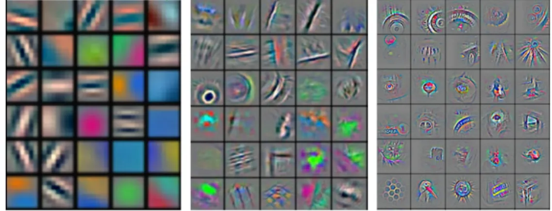
Figure 1.4: The learned representations are from coarse to ne [127].
Deep learning is part of the boarder family of representation learning which learns multiple levels of data representations by stacking non-linear layers that each transforms the
representation from a lower and coarser level into one at higher and ne level. For a specic task, high level layers of representation amplify aspects of the input that are important for discrimination and suppress irrelevant variations [63]. As shown in Fig. 1.4, the CNN takes an image of a Samoyed as input which is represented as three channels of pixel arrays, and the learned low level features typically describe edges at particular orientations and locations in the image. For high level layers, abstract of the whole images is extracted and then used for specic tasks. The most signicant advantage of deep learning is that data representation is learned with a general purpose learning framework instead of being designed by human engineers [63].
Deep learning frameworks have turned out to be very good at discovering intrinsic structures in high dimensional data and are therefore applicable to many domains of science. In addition to overperforming state-of-the-arts in image recognition [58, 31, 21] and speech recognition [96, 83], deep learning also produced extremely promising results for various tasks in natural language understanding [54], question answering [4] and machine translation [7, 106].
Our Contributions
In this dissertation, we focus on representation learning with deep neural networks. Specically, we propose the following research topics with signicant intellectual merit and novelty. We summarize below the three research projects that we accomplished as part of this dissertation.
Learning topic-based word embedding for text analysis
We propose a novel word embedding learning approach, which provides topic-based semantic word embeddings and two CNN architectures, that can utilize multiple word rep-resentations simultaneously for text classication. Specically, the main contributions are summarized as follows:
• We develop a word embedding learning model, Topic-based Skip-gram, which
cap-tures word semantic relationship with topic models, e.g., LDA, and then integrate it into distributed word embedding learning with a novel objective function.
• We introduce two complementary multimodal CNN architectures that
simultane-ously take multiple kinds of word embeddings as inputs for text classication.
• We combine the proposed topic-based word embedding and other state-of-the-art
word embeddings as inputs to the proposed multimodal CNN architectures. Our experiments conducted on several real-world datasets show that combination of the proposed topic-based word representations and our multimodal CNNs outperforms state-of-the-art word represen-tations in various text classication tasks, including indexing of biomedical articles.
Learning 3D polygon representation for shape segmentation
We propose Directionally Convolutional Network that extends convolution operations from images to the surface mesh in the spatial domain. Furthermore, we introduce a two-stream framework combining proposed Directionally Convolutional Network and a neural network for segmentation of 3D shapes. Instead of fusing the two streams by a simple con-catenation, we take our framework as an approximation of a directed graph and combine the probabilities inferred by the two streams with an element-wise product. Finally, Conditional Random Field is applied to optimize the surface mesh segmentation. The main contributions are summarized as follows:
•By dening rotation-invariant convolution and pooling operations on the surface of
3D shapes, we learn eective shape representations from raw geometric features, i.e., face normals and distances, to achieve robust segmentation of 3D shapes.
• Based on the proposed Directionally Convolutional Network, we introduce a
two-stream framework to classify each face of a given mesh into predened semantic parts. Our approach achieves state-of-the-art segmentation results on a large variety of 3D shapes.
Learning deep brain ber representation for classication
We propose a CNN-based end-to-end learning framework with direct representation learning to dierentially delineate diusion tensor imaging (DTI)-based eloquent axonal pathways by incorporating functional MRI (fMRI) and electrical stimulation mapping (ESM) observations. The main contributions of this work are as follows:
• Two CNN architectures with dierent depth were investigated in this study: a
shallow CNN model with3layers from our previous work [119]; inspired by the great success
of very deep CNNs [41, 92], we also adapted the shallow CNN into a deep model with 21
layers. The proposed CNN models generate dierent feature maps of the input data (i.e., 3D spatial coordinates of individual ber streamlines) by using a sequence of convolutional and pooling layers before classifying input data using fully connected layers.
• A couple of novel CNN loss functions [68, 116] were introduced for pathway
clas-sication task. First, since our dataset is highly unbalanced, which cannot be handled well by CNN with the conventional cross-entropy loss, we introduced focal loss into the proposed CNN models. Focal loss applies a modulating term to the cross-entropy loss to help focus on hard examples and down-weight the numerous easy examples. Second, to further im-prove the classication performance and generalization ability of proposed CNN models, the learned ber representations need to be not only separable but also discriminative. Center loss was introduced which adds a cluster-based loss term to the cross-entropy loss to ensure the learned representations have both compact intra-class variations and large inter-class margins.
•Although CNNs have led to breakthroughs of state-of-the-arts, the end-to-end
learn-ing strategy makes the entire CNN model a black box. This weakness is highlighted in the biomedical imaging: if we do not know how the trained CNNs classify each ber, we cannot fully trust the classication results given by the CNN models. In this study, we applied attention mechanism [120] in the proposed CNNs, which highlights the most useful segments of a ber for classication. In this study, we will demonstrate that the attention
mecha-nism provides a machine perspective on how the CNNs classify functionally-important white matter pathways.
Organization
The rest of this dissertation is organized as follows: In Chapter 2, we introduce our method on learning topic-based word embedding for text analysis. In Chapter 3, we describe the proposed approach to learning 3D polygon representation for shape segmentation using a two-stream deep neural network framework. In Chapter 4, we introduce our framework to learn eective, discriminative, and interpretable brain ber representations for classication in detail. In Chapter 5, we conclude and review future research directions.
CHAPTER 2 Learning Word Embedding for Text Analysis
In this chapter, we propose a novel neural language model, Topic-based Skip-gram, to learn topic-based word representation for text analysis with CNNs. Topic-based Skip-gram leverages textual content with topic models, e.g., Latent Dirichlet Allocation, to capture precise topic-based word relationship and then integrate it into distributed word embedding learning. We then describe two multimodal CNN architectures, which are able to employ dierent kinds of word embeddings at the same time for text classication.
Introduction
As the amount of biomedical textual data in MEDLINE of the US National Library of Medicine (NLM) is growing exponentially, the indexing of biomedical articles is becoming a much more dicult task. Medical Text Indexer (MTI)1 [5] has been assigned to this task as a support tool which produces (semi-)automated recommendation indexing based on predened Medical Subject Headings (MESH)2. Meanwhile, biomedical literature indexing can also be viewed as a classication over textual data into a set of predened classes. However, as discussed in [93, 124], traditional machine learning algorithms, including Naive Bayes, Support Vector Machine and Logistic Regression, cannot outperform MTI system without ensemble.
Recently, CNN models have achieved remarkably strong performance in natural lan-guage processing and become commonly used architectures for text classication [49, 54, 60, 128]. As input features of CNNs, various types of word vector representations have been proposed. Generally speaking, there are two model families to represent words with real-valued vectors: 1)matrix factorization methods, such as [28, 71] and 2)local window-based methods, such as [12, 25, 78]. Both families have their own pros and cons. Although matrix factorization methods do not require much domain expertise of word embedding and e-ciently leverage statistical information of corpora, their main problem is that most frequent words (or characters) have a large negative impact on word similarity measure, which leads
1http://ii.nlm.nih.gov/MTI/index.shtml
to poor performance on word analogy tasks. Local window-based methods perform better on analogy tasks, but they poorly utilize statistical information about corpus because these models are trained on separate local windows of content.
In the presented work, we propose a novel word embedding learning approach, which provides topic-based semantic word embeddings and two CNN architectures, which can uti-lize multiple word representations simultaneously for text classication. Specically, our framework rst leverages the whole text corpus with topic models to capture semantic re-lationship between words and then take it as the input for word representation learning using Topic-based Skip-gram with a novel objective function. Then, these topic-based word representations are used together with other state-of-the-art word embeddings for text clas-sication in multimodal CNN models. Specically, the main contributions of this work are summarized as follows:
•We propose a learning-based word embedding model, Topic-based Skip-gram, which
captures word semantic relationship with topic models, e.g., LDA, and then integrate it into distributed word embedding learning with a novel objective function.
•We introduce two complementary multimodal CNN architectures that are able to
simultaneously take multiple kinds of word embeddings as inputs for text classication.
• We combine the proposed topic-based word embedding and other state-of-the-art
word embeddings as inputs to the proposed multimodal CNN architectures. Our experiments conducted on several real-world datasets show that combination of the proposed topic-based word representations and our multimodal CNNs outperforms state-of-the-art word represen-tations in various text classication tasks, including indexing of biomedical articles.
The rest of this chapter is organized as follows. In Section , we review related work in biomedical literature indexing and word representation learning. The details of our word embedding learning approach and multimodal CNN models are introduced in Section . In Section , we demonstrate that our topic-based word embedding produces competitive results
with CNN architecture and outperforms state-of-the-art approaches with our multimodal CNN models in three case studies. At last, we conclude in Section .
Related Work
Indexing of Biomedical Literature
Our work shares the high-level goal of biomedical literature indexing with many pre-vious works, such as USI [33], MeSHLabeler [69], MeSH Now [73] and Atypon [84]. Several other works [93, 124] tried to improve the MTI system with automatic machine learning methods. Among them, Yepes et al. [124] pointed out that ensemble of classic machine learning methods can outperform indexing performance of MTI. Rios and Kavuluru [93] surpassed MTI performance by utilizing CNNs for sentence-level textual classication [54] with word embeddings trained by the Skip-gram model [78], which is more closely related to our work. However, these works focus on utilizing classic machine learning methods for biomedical literature indexing, while we propose a novel Topic-based Skip-gram for learning topic-based semantic word representations and obtain state-of-the-art classication perfor-mance with deep learning architectures.
Topic Models
Topic models are probabilistic generative models to discover main themes of docu-ments. These models share the same assumptions: 1) they posit there are a set of latent topics, which are multinomial distributions over vocabulary; 2) each document is a mixture of these topics. Recently, topic models have become a popular tool for text classication [75, 90], image classication [32, 91], transfer learning [20, 121] and unsupervised analysis of textual data [14, 15]. As one of the most commonly used unsupervised topic models, Latent Dirichlet Allocation (LDA) [15] can extract semantic information from corpora. The basic assumption of LDA is that each document is a mixture of topic proportions and each topic is a distribution over xed vocabulary. In this work, we employ LDA to identify topic-based semantic relationships between words in each corpus.
Word Embedding Learning Methods
Recently, Mikolov et al. introduced an algorithm for learning xed length distributed representations of words in a vector space, the Skip-gram model [77], which is a single-layer neural network based on inner products between word vectors. As one of the local window-based methods, Skip-gram's objective is to learn word embeddings that can predict the textual content of a word given the word itself. Through experiments on word and phrase analogy tasks, this model demonstrated its capacity to capture linguistic relationships between word vectors. However, Skip-gram model suers from the disadvantage that it does not utilize the co-occurrence statistics of the corpus. Instead, Skip-gram scans textual corpus with local context windows, which fails to make use of statistical information of the whole corpus. Pennington et al. [87] took the advantages of both global matrix factorization and local content window-based methods by training their model only on nonzero elements in the word co-occurrence matrix. Dierent from their approach, Topic-based Skip-gram leverages global statistical information of the whole corpus with LDA and learns the semantic information with local content windows.
CNNs for Text Classication
A number of CNN architectures have been developed for text classication [49, 54, 60, 128]. Kalchbrenner et al. [49] focused on sentence modeling with a CNN-based model for word-level input. Zhang and LeCun [128] concentrated on character-level input with a very deep CNN architecture which requires a large amount of training data and training time. Lai et al. [60] proposed a model which combines Recurrent Neural Networks (RNN) with CNN. Kim [54] proposed a two-layer CNN model for sentence-level text classication with single kind of word embeddings. This model is simple but very eective for text classication. Our multimodal approach is inspired by this model. In contrast to the architecture described by Kim, our multimodal approaches are able to simultaneously take multiple kinds of word representations as inputs.
The Proposed Approach
In this section, we rst present technical details of Topic-based Skip-gram for learning topic-based semantic word embeddings and then introduce two multimodal CNN architec-tures which employ multiple kinds of word embeddings as inputs for text classication.
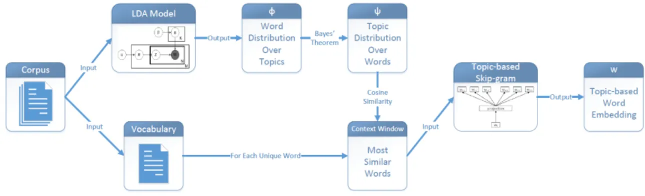
Figure 2.1: Workow of Topic-based Skip-gram.
Topic-based Skip-gram
Topic-based Skip-gram identify semantic relationship between words from corpus us-ing LDA and then integrate it into word representation learnus-ing with a novel objective function. The workow is shown in Fig. 2.1 and we will introduce the details in this subsec-tion.
Leveraging Topic-based Semantic Information with LDA
LDA. The basic idea of LDA is that each documentd is a distribution overK latent topics and each topic is a distribution overV unique words in the dictionary. Given a corpus of M documents and each document has Nm words, the generative process of LDA is as
follows:
1. Choose θ ∼Dirichlet(α)
θ denotes topic distribution over documents. Each document has its own θ, which needs to be estimated during the training stage. Eachθ is a vector of length K, where K is the number of topics and chosen manually at the beginning of training. α is the hyperparameter of document-topic distribution.
2. Choose φ∼Dirichlet(β)
φ is word distribution over topics, also known as topic in [15], which is a matrix of K rows and V columns. Element φi,j equals p(wj|zi), which is the probability of
generating wordwj given this word belonging to topic zi. β is the hyperparameter of
topic-word distribution.
3. For each of the N words wn in each document dm of the M documents in the corpus:
(a) Choose a topic zn ∼Multinomial(θ)
The topic indicator zn is the topic k assigned to word wn.
(b) Generate a word wn ∼Multinomial(zn,β)
Generate a word as wn, which is the nth unique word in the dictionary, from
Multinomial distributionp(wn|zn,β).
Topic-based Semantic Information of Corpus. In this chapter, we treat the topic distribution over words ψ as topic-based semantic information of corpus for learning word embeddings. ψ is a V ×K matrix. Its element ψi,j is equal to p(zi|wj), which is
the probability for word wj to be assigned to topic zi. It can be approximated with word
distribution over topics φ based on Bayes' theorem: p(zi|wj) =
p(wj|zi)·p(zi)
p(wj)
, (2.1)
wherep(zi)is the marginal probability of topicziandp(wj)denotes the marginal probability
of wordwj in the dictionary. p(zi)and p(wj) can be calculated as follows:
p(zi) = PM m=1z m i M , (2.2) p(wj) = PM m=1Nmj PM m=1Nm , (2.3)
where zmi is the topic proportion of zi in document dm and Nmj is the count of word wj in
the document dm. The topic-based semantic information matrix ψ is then used as training
data in the word embedding learning step. Learning Topic-based Word Embeddings
Skip-gram. The training objective of Skip-gram [78] is to learn distributed word representations which aim at predicting the surrounding words in the documents. Given a training corpus ofT words w1, w2, w3,· · · , wT, the learning objective of the Skip-gram model
is to maximize the average log probability
1 T T X t=1 X −c6j6c,j6=0 logp(wt+j|wt), (2.4)
wherec is the size of training content. In other words, given a local window of size2·c+ 1,
the objective of Skip-gram model is to maximize prediction log probability of the 2·cwords wt−c, wt−c+1,· · · , wt−1, wt+1,· · · , wt+c−1, wt+c given the word wt in the center.
Learning Semantic Word Embeddings. We propose a novel training objective function for Topic-based Skip-gram that is to learn distributed word embeddings which are useful to predict words with similar topic-based semantic information. The basic assumption of Topic-based Skip-gram is that if topic distributions of two wordsψi and ψj have a large
cosine similarity between each other, then these two words share similar topic-based semantic information. Given a dictionary of N unique words w1, w2, w3,· · · , wN of a corpus, the
objective of Topic-based Skip-gram model is to maximize the average log probability
1 N N X n=1 X −c6j6c,j6=0 logp(wn+j|wn). (2.5)
In other words, given half window size c (s.t. window size is 2c+ 1) and a word in the
dictionarywn, the training objective of Topic-based Skip-gram is to maximize prediction log
sof tmax function p(wn+j|wn) = exp(vw>n+jvwn) P 16i6N,i6=nexp(v>wivwn) , (2.6)
where vwn is the vector representation of word wn. In practice, the cost of computing
Ologp(wn+j|wn)∝N, whereN can be very large (106−108 unique words).
Optimization. Same with Skip-gram, we use Negative Sampling [78] to optimize the objective function of Topic-based Skip-gram. In Negative Sampling, p(wn+j|wn) is replaced
as logσ(wn+j|wn) + k X i=i Ewi∼Pn(w)[logσ(−v > wivwn)]. (2.7)
The idea is to distinguish target word wn+j fromk noise words which are drawn from noise
distribution Pn(w) using logistic regression by maximizing the probability of target word
(rst item) and minimizing the probability of noise words (second term). According to results reported in [78], we choose k = 15 and Pn(w) ∼
U(w)0.75
Z ,where U(w) is unigram distribution.
Time eciency. Given a dataset ofN unique words andLwords in total, proposed Topic-based Skip-gram optimizes N word windows and Skip-gram optimizes L windows. Note that N L in most cases. Furthermore, Topic-based Skip-gram can also work with other semantic indexing models in addition to LDA, which may signicantly expedite the training process.
We summarize the learning procedure for topic-based semantic word embedding in Algorithm 1.
Multimodal CNN Architectures
In this part, we rst introduce a single channel CNN model [54], which is used as baseline architecture in the experiments. Then we will describe the two proposed multimodal CNN architectures which can take multiple types of word embeddings with dierent length.
Algorithm 1 Topic-based Skip-gram
1: Input: Raw training textual corpus D; Topic number K, Hyperparameters α,β for LDA, Half window size c
2: Output: Topic-based semantic word embedding W 3: procedure GetWordEmbedding
4: φ=LDA(D,α,β, K) . Train LDA model on the corpus D and get word
distribution over topics φ
5: for Each topic zi do
6: Compute marginal probability of each topic p(zi)with Eq. (2.2)
7: for Each word wj do
8: Compute marginal probability of each wordp(wj) with Eq. (2.3)
9: Compute topic distribution over words ψ based on Eq. (2.1), (2.2) and (2.3)
10: for Each word wj do
11: Find2cwords with most similar topic distribution over words towj according to
cosine similarity .These 2c+ 1 words are then used as an input window winj for
Topic-based Skip-gram
12: W=Topic-based-Skip-gram(win) .Take all word windows win as input of Topic-based Skip-gram to learn topic-based word embedding W based on the objective
function in Eq. (2.5) Baseline CNN
The baseline CNN contains one input layer, one convolution layer, one maxpooling layer and one fully connected layer. Although one output neuron with sigmoid or tanh function is sucient for binary classication, we choose multiple neurons with sof tmax function to make it easier to adopt CNN models for multi-class classication. The details of each layer are described as follows.
Input layer. Formally, we denote xi ∈Rk as thek-dimensional word representation for the ith word in a sentence. A sentence of length n is denoted as
X1:n =x1⊕x2⊕ · · · ⊕xn, (2.8)
where⊕is the concatenation operator. By this, each input sentence is represented as an×k matrix. In practice, short sentences are padded with zeros to same length, such that, each matrix shares the same size.
Convolution layer. A convolution lterw∈Rh×k, which is applied to a window of
hwords ofk-dimensional embeddings, produces a new feature. For instance, given a window of words Xi:i+h−1 and a bias term b∈R, a new feature ci is generated by
ci =f(w·Xi:i+h−1+b), (2.9)
where f is a non-linear function. In our case, we apply the element-wise function Rectied Linear Unit (ReLU) to the input matrices:
ReLU(x) = x, if x >0 0, otherwise (2.10)
Each lter produces a feature map c = [c1, c2,· · · , cn−h+1] from every possible window {X1:h,X2:h+1,· · · ,n−h+1:n}of a sentence of lengthn. In [54], multiple layers of various sizes are applied in the convolution layer, and multiple feature maps are generated.
Sub-sampling layer. There are several sub-sampling methods, such as average pooling, median pooling and max pooling. In this case, we apply max pooling over each feature map produced by the convolution layer and take the maximum elementˆc=max{c}.
Let's denote features generated by this max pooling layer as
ˆc= ˆc1⊕ˆc2⊕ · · · ⊕cˆm, (2.11)
where m is the number of feature maps.
Fully connected layer. Givenˆc as the input, the fully connected layer produces
where Y is the prediction, θ denotes parameters {W, b}, W denotes weights, ◦ denotes
the element-wise multiplication operator and r∈ Rm is a dropout mask vector of Bernoulli
variables with probabilitypof being zero. During the back propagation stage, only unmarked elements inˆcare involved in the computation. l2-norm [44] is also applied to weight matrices
W. If kWk2 > s after gradient descent step, we rescale W, such that kWk2 =s. Here, s is a manually dened parameter. By applying dropout andl2-norm, we prevent the overtting
problem.
Optimization. A reasonable training objective is to minimize categorical (or binary) cross-entropy loss. The average loss for each sample is
Q(θ) = 1 |D|L(θ,D) =− 1 |D| |D| X i=1 logP(Y =yi|xi,θ), (2.13)
where xi is the ith sample in the dataset and yi is the prediction for it. In the proposed framework, we update the parameters θ by Adadelta [126], which is an adaptive learning rate approach for classic SGD.
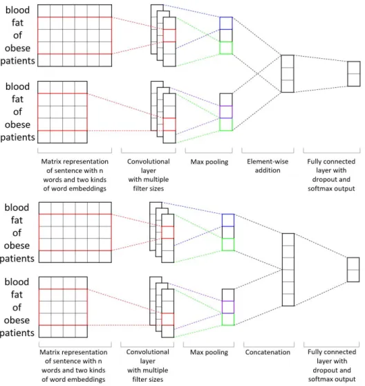
Multi-channel CNN (CNN-channel)
As shown in the top panel of Fig. 2.2, CNN-channel model combines two baseline CNN models. More formally, we denote two kinds of word embeddingsx1i ∈Rk1 andx2
i ∈R
k2
ask1- andk2-dimensional word representations for theith word in a sentence. So, a sentence
of length n can be represented in two ways
X11:n =x11⊕x12⊕ · · · ⊕x1n (2.14)
and
where X11:n is used as the input matrix for the `top channel' of CNN-channel and X21:n is
the input for the `bottom channel' of CNN-channel. Similarly, after applying convolution and max-pooling layers, ˆc1 and ˆc2 are generated. In CNN-channel, they are merged by
element-wise addition:
ˆc=ˆc1 +ˆc2 (2.16)
Here,+denotes element-wise addition. Then we apply the fully connected layer with dropout
and softmax output and l2 regularization as in the baseline CNN model.
Concatenation CNN (CNN-concat)
As shown in the bottom panel of Fig. 2.2, CNN-concat is also built on top of the baseline CNN model. Dierent from CNN-channel,ˆc1 and ˆc2 are merged by concatenation
ˆc=ˆc1 ⊕ˆc2 (2.17)
Thenˆcis taken as the input of fully connected layer as in the baseline CNN model. Although
CNN-channel and CNN-concat models can be expended to utilize as many types of word embeddings as needed, we only employ two kinds of word representations in our experiments. Deep Understanding of Multimodal CNNs
Multimodal CNNs vs. original CNN model. Original CNN architecture, which was proposed in [54], can only take one kind of word embedding as input. Meanwhile, our proposed multimodal CNNs are able to simultaneously take multiple types of word embeddings as inputs, which means that multimodal CNNs have stronger learning ability than the original CNN model. Specically, by combing the topic-based word embedding and local window-based word embeddings, the multimodal CNNs are able to utilize both topic-based semantic relationship and local content information and outperform the original CNN model.
CNN-channel vs. CNN-concat. CNN-channel combines the two kinds of word representations by element-wise addition, commonly used for multi-channel image classi-cation. On the other hand, CNN-concat concatenates two parts together, which introduces more parameters to t. In other words, CNN-concat has stronger learning ability but needs more training data to preserve from overtting than CNN-channel. When the training set has enough positive samples for binary classication task or is balanced for multi-class clas-sication problem, CNN-concat is a better choice than CNN-channel.
Experiments
We evaluate our framework by three tasks: 1)indexing of biomedical articles; 2)an-notation of clinical text fragments with behavior codes; and 3)classication of benchmark newsgroups. Baselines and state-of-the-art algorithms are compared with our method in these experiments. In our experiments, we used the same code3 and parameter settings as in [93] for the baseline CNN model. We make implementation of proposed multimodal CNNs publicly available4.
Datasets
Indexing of Biomedical Articles
MEDLINE citations. A public dataset5 of MEDLINE citations from November 2012 to February 2013 is used in this work. The dataset contains 143,853 citations in total, from which 94,942 citations were selected for training and 48,911 were selected for testing. As in [93], we categorize 29 MeSH terms into three groups according to MTI's performance: check tags, low precision terms and low recall terms. The check tags group is a common set of top 12 MeSH headings routinely considered for almost all articles (e.g. Humans, Female and Male), the low precision group contains 10 MeSH headings with the lowest precision performance using MTI and the low recall group contains 7 MeSH headings with the lowest recall performance using MTI. We build CNN models as binary classiers for each MeSH to
3https://github.com/yoonkim/CNN_sentence
4https://github.com/HaotianMXu/Multimodal-CNNs
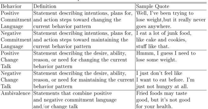
Table 2.1: Description of ve behavior code annotations.
Behavior Denition Sample Quote
Positive Statement describing intentions, plans for, Well, I've been trying to Commitment and action steps toward changing the lose weight,but it really never
Language current behavior pattern goes anywhere.
Negative Statement describing intentions, plans for, I eat a lot of junk food, Commitment and action steps toward maintaining the like cake and cookies,
Language current behavior pattern stu like that.
Positive Statement describing the desire, ability, Hmmm, I guess I need to Change reason, or need for changing the current lose some weight.
Talk behavior pattern
Negative Statement describing the desire, ability, I just don't feel like Change reason, or need for maintaining the current I want to eat before. I'm
Talk behavior pattern just not hungry at all.
Ambivalence Statements that combine positive Fried foods may taste and negative commitment language good, but it's not good
and/or change talk for your health.
classify if a document belongs to this MeSH term. Note that although only 29 terms are used in this experiment, our framework works for arbitrary number of MeSH terms.
Annotation of Clinical Text Fragments with Behavior Codes
Clinical interview fragments. As discussed in [57], behavior code annotation can be treated as a classication problem which assigns a code to each utterance. We use a collection of motivational interviewing-based weight loss sessions, which consists of 11,353 utterances that were manually annotated by two human coders as a golden standard. On top of this dataset, we conduct three behavior code annotation tasks: A) Positive, Negative and Ambivalence; B) Commitment Language, Change Talk and Ambivalence; C) Positive Commitment Language, Negative Commitment Language, Positive Change Talk, Negative Change Talk and Ambivalence. The description of behavior code is listed in Table 2.1. Classication of News Groups
20 Newsgroups. This publicly available6 dataset[61] has been widely used to evalu-ate text classication algorithms. The 20 Newsgroups dataset is a collection of approximevalu-ately
20,000 newsgroup documents across six categories, i.e., computers, recreation, science, pol-itics, religion and forsale. In this work, we use four most common classes, which are com-puters, recreation, science and politics, as a four-class classication task to evaluate our framework.
Methods Compared
Baseline Approaches
The following non-CNN models are used as our baseline:
• MTI. Medical Text Indexer, which is commonly used in biomedical literature
in-dexing. We only compare our method with MTI in the indexing task of biomedical articles.
•Prior-best. Prior-best is the best-performed method in the experiments of several
classic machine learning methods, including Naive Bayes(NB), Logistic Regression(LR) and Support Vector Machine(SVM). For indexing of biomedical articles, Support Vector Machine with Huber Loss (SVM HL) [123] is also compared.
CNN-based Methods
In our experiments, we compared Topic-based Skip-gram with several baseline and state-of-the-art distributed word embedding learning methods, including:
•CNN-rand. Each word embedding is initialized with values drawn from continuous
uniform distribution U ∼ [−0.25,0.25]. CNN-rand is used as a baseline of CNN-based
methods.
•CNN-gn. These word vectors were trained by Mikolov et al. [78] on Google News
and are publicly available7. • CNN-glove. The word embeddings used in this work were trained by Pennington et al. [87] 8.
• CNN-local. The word representations are trained by Skip-gram on the datasets
to classify. The implementation of Skip-gram is publicly available9.
7https://code.google.com/archive/p/word2vec/
8http://nlp.stanford.edu/projects/glove/
• CNN-topic. These word embeddings are learned by our Topic-based Skip-gram
on the datasets to categorize.
These kinds of word embeddings are compared under the baseline CNN architecture. Our two multimodal CNN architectures are also compared in this work:
•channel. We utilize two kinds of word embeddings for channel,
CNN-local and CNN-topic.
• CNN-concat. CNN-local and CNN-topic are employed for CNN-concat.
We also tried to combine CNN-gn and CNN-glove with CNN-topic for multimodal CNN models, but their classication performance is not as good as combination of CNN-local and CNN-topic. The reason is that there are quite a few appeared words not in the CNN-gn and CNN-glove vocabulary, and embeddings for these words need to be randomly initialized. For example, more than 60% of words in the vocabulary of MEDLINE citations
are not in the pre-trained CNN-glove vocabulary and need to be randomly initialized. This signicantly and negatively impacts the performance of CNN-gn and CNN-glove.
Metrics
In this work, we use F1 score to evaluate the performance of binary classiers and
macro-averaged F1 score for multi-class classiers.
F1 score
F1 score is a measure of binary classication accuracy, which is robust to unbalanced
data distribution: F1 = 2×
precision×recall
precision + recall, (2.18)
where precision is ratio of instances which are classied as positive are correct and recall is the ratio of positive instances that are correctly classied.
Table 2.2: F1 scores for check tags group.
MeSH Positive Prior CNN CNN CNN CNN CNN CNN CNN
Term best rand gn glove local topic channel concat
Adolescent 3824 0.4144 0.4321 0.4311 0.2677 0.4382 0.4104 0.4321 0.4437 Adult 8792 0.5700 0.6095 0.6192 0.5389 0.6159 0.6121 0.6354 0.6278 Aged 6151 0.5614 0.5695 0.5705 0.4378 0.5568 0.5645 0.5841 0.5737 Aged, 80 and over 2328 0.3227 0.321 0.3406 0.0642 0.3231 0.3316 0.3428 0.3639 Child, Preschool 1573 0.4954 0.4998 0.5126 0.4270 0.4944 0.4909 0.5363 0.5289 Female 16483 0.7517 0.7644 0.7761 0.7169 0.7761 0.7784 0.7810 0.7840 Humans 35967 0.9269 0.9307 0.9360 0.9113 0.9365 0.9351 0.9366 0.9361 Infant 1281 0.4441 0.4642 0.5032 0.1296 0.4923 0.4957 0.5262 0.5206 Male 15530 0.7294 0.7469 0.7477 0.6822 0.7631 0.7561 0.7543 0.7545 Middle Aged 8392 0.6377 0.6558 0.6665 0.6076 0.6692 0.6784 0.6803 0.6759 Swine 285 0.7071 0.7190 0.7332 0.6252 0.7406 0.7444 0.7539 0.7496 Young Adult 3807 0.3371 0.3125 0.3238 0.0499 0.3389 0.3128 0.3229 0.3652 Macro-averaged F1 score
For multi-class classiers, we employ macro-averaged F1 score to evaluate their
per-formance, which is an arithmetic average ofF1 score for each class:
Macro-averaged F1 = 1 n n X i=1 F1i, (2.19)
where n is total number of classes and F1i is F1 score for ith class.
Experimental Results
In this section, we report the experimental results of baselines, state-of-the-art meth-ods and our topic-based word embedding and multimodal CNN models. Best results are marked in bold.
Results of Indexing of Biomedical Articles
F1 scores of each method over the check tags group, the low precision group and
the low recall group are listed in Table 2.2, 2.3 and 2.4, respectively. The Positive column shows the number of positive samples for each MeSH. The results of MTI and Prior-best were reported in [93]. Although no single method outperforms all of the other approaches, the following observations can be made.
Table 2.3: F1 scores for low precision MeSH group.
MeSH Positive MTI Prior CNN CNN CNN CNN CNN CNN CNN
Term best rand gn glove local topic channel concat
Age Factors 889 0.0844 0.1450 0.2150 0.2212 0.0001 0.2142 0.2233 0.2206 0.2429 Brain 823 0.5201 0.4182 0.4300 0.4596 0.1902 0.4226 0.4571 0.4697 0.4821 Cell Line 781 0.2876 0.2265 0.2277 0.2139 0.0721 0.3009 0.2389 0.2704 0.3212 Cells, Cultured 1079 0.3046 0.2784 0.2457 0.2936 0.0841 0.2807 0.2723 0.3350 0.2739 Models, 851 0.4292 0.3734 0.3769 0.4283 0.2282 0.3893 0.4138 0.4209 0.4307 Molecular Molecular 1527 0.5495 0.4094 0.3863 0.4035 0.2141 0.4140 0.3532 0.4211 0.4024 Sequence Data RNA, 628 0.4477 0.4385 0.4421 0.4397 0.3110 0.3918 0.4374 0.4576 0.4486 Messenger Severity of 751 0.1824 0.1924 0.1598 0.2106 0.0372 0.1588 0.2106 0.1927 0.2237 Illness Index Time Factors 2153 0.098 0.1393 0.091 0.1188 0.0221 0.1123 0.1179 0.1401 0.1364 United States 2658 0.3585 0.3655 0.4128 0.4599 0.1081 0.4213 0.4292 0.4791 0.4653
Table 2.4: F1 scores for low recall MeSH group.
MeSH Positive MTI Prior CNN CNN CNN CNN CNN CNN CNN
Term best rand gn glove local topic channel concat
Child 2780 0.5863 0.5723 0.6015 0.6099 0.5488 0.6102 0.6040 0.6180 0.6192 Follow-Up 1470 0.0407 0.2300 0.2189 0.2368 0.1187 0.2247 0.2284 0.2514 0.2264 Studies Reproducibility 1206 0.3191 0.3138 0.2963 0.3220 0.1921 0.3261 0.3110 0.3147 0.3274 of Results Retrospective 2183 0.6608 0.6580 0.6647 0.6578 0.6346 0.6585 0.6617 0.6754 0.6589 Studies Risk Assessment 1014 0.2556 0.1610 0.2063 0.1854 0.1411 0.2145 0.1979 0.2100 0.2298 Risk Factors 2365 0.4989 0.3778 0.4438 0.4510 0.3446 0.4711 0.4514 0.4654 0.5003 Treatment 2999 0.4202 0.3859 0.3635 0.3590 0.2274 0.3752 0.3592 0.3831 0.3876 Outcome
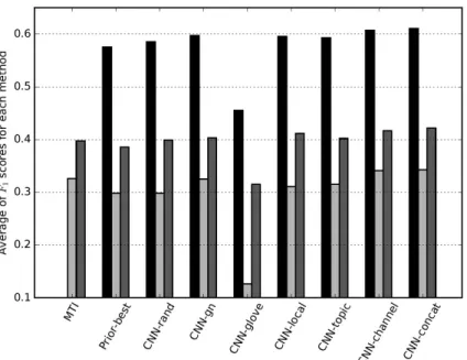
Figure 2.3: Macro-averaged F1 scores of each method from the three groups.
First, CNN-channel and CNN-concat give the best performance for more than82.7%
selected MeSH terms. Only for four MeSH terms: Brain, Molecular Sequence Data, Risk Assessment and Treatment Outcome, MTI system demonstrates better results than the proposed multimodal CNNs.
Second, our multimodal CNN architectures outperform baseline CNN models with a single type of word embedding. This is mainly because multimodal CNNs utilize topic-based semantic word embedding as well as local content-based embedding. According to results shown in Table 2.2, 2.3 and 2.4, introducing topic-based semantic information improves indexing results.
Third, CNN-concat gives better results than CNN-channel for 15 terms among 29
terms and CNN-concat performs better than CNN-channel for more balanced MeSH terms. Considering there are 94,942 training samples in total, most MeSH terms are highly imbal-anced. Among the 13 more balanced terms (Positive samples : Negative samples >0.025 : 1),
CNN-concat performs better than CNN-channel for eight MeSH terms and the average F1
Fourth, baseline CNN model with our proposed topic-based word embedding produces competitive results with gn and local. Word vectors used in gn and CNN-local are both trained with Skip-gram, which is the state-of-the-art word representation learning approach.
Fifth, CNN-glove demonstrates poor performance. The reason is that more than
60% of unique words in MEDLINE are not in the CNN-glove vocabulary and need to be
randomly initialized. CNN-glove is pre-trained on Wikipedia2014 and Gigaword5 which do not contain many technical terms in biomedical domain. We can see that CNN-glove gives better performance on clinical text fragments and newsgroups datasets because more unique words are contained in the pre-trained vocabulary.
Sixth, the Prior-best columns refer to the best F1 scores for traditional machine
learning algorithms which give worse performance than CNN-based models. It indicates that CNN-based approaches are more eective for indexing problems than NB, LR, SVM and SVM HL.
Finally, we summarize average ofF1 scores for each method in all of the three MeSH
term groups in Fig. 2.3. Although there is no model outperforming all of the other models, CNN-concat demonstrates the best overall performance and CNN-channel gives very com-petitive average F1 scores. Further, word embedding learned by our proposed Topic-based
Skip-gram produces state-of-the-art results with baseline CNN model. Results of Behavior Code Annotation of Clinical Text Fragments
Three cases of multi-class behavior code annotation are conducted for this task: case
1, annotation over positive, negative and ambivalence, with sample ratio 1 : 0.014 : 0.150;
case 2, annotation over commitment language, change talk and ambivalence, with sample
ratio 0.527 : 1 : 0.094; case 3, annotation over positive commitment language, negative
commitment language, positive change talk, negative change talk and ambivalence, with sample ratio 0.067 : 0.573 : 0.214 : 1 : 0.114. Clearly, all of these three data splits are
Figure 2.4: Macro-averaged F1 scores for clinical text fragments.
macro-averaged F1 scores for all methods over ve folds. As shown in Fig. 2.4,
CNN-channel gives the best F1 scores among all the compared methods in the three cases and
CNN-concat produces comparable results, which shows that CNN-channel performs better than CNN-concat for classication on highly imbalanced datasets. For word representation learned with baseline CNN models, CNN-topic, which is trained with proposed Topic-based Skip-gram, demonstrates better performance than other state-of-the-art word embeddings. Prior-best, which includes NB, LR and SVM in this task, is less eective than all CNN-based models.
Results of Classication of Newsgroups
This task is a 4-class classication problem over computers, recreation, science and
politics. The sample ratio of the four categories is 1 : 0.876 : 0.811 : 0.668, which is
roughly balanced. 5-fold cross validation is applied to the whole dataset and the average
macro-averaged F1 scores over the ve folds are reported in Fig. 2.5. First, CNN-channel
and concat outperform other baselines and state-of-the-art methods. Second, CNN-concat demonstrates better performance than CNN-channel on this balanced dataset. Third, CNN-topic with baseline CNN model produces a comparableF1score with other
state-of-the-Figure 2.5: Macro-averaged F1 scores for news groups.
art word embeddings. Furthermore, CNN-based models signicantly outperform non-CNN models (NB, LR and SVM).
Conclusion
In this chapter, we proposed a novel framework,Topic-based Skip-gram, for learning topic-based semantic word embeddings for text classication with CNNs and achieved highly competitive results with word embeddings learned by Skip-gram. While Skip-gram focuses on context information from local word windows, the proposed Topic-based Skip-gram leverages semantic information from documents.
We also described two multimodal CNN architectures, CNN-channel and CNN-concat, which can ensemble dierent kinds of word embeddings. CNN-channel has a better imbal-anced data resistance than CNN-concat, while CNN-concat has stronger learning ability and performs better on more balanced datasets.
Through experiments on indexing biomedical literature, annotation of clinical text fragments with behavior codes and text classication of a textual benchmark, we showed that our topic-based semantic word embeddings with multimodal CNNs outperform state-of-the-art word representations in text classication.
CHAPTER 3 Learning 3D Representation for Segmentation
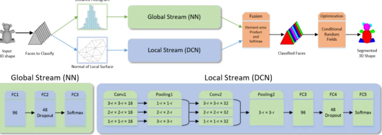
Previous approaches on 3D shape segmentation mostly rely on heuristic processing and hand-tuned geometric descriptors. In this chapter, we propose a novel 3D shape repre-sentation learning approach, Directionally Convolutional Network (DCN), to solve the shape segmentation problem. DCN extends convolution operations from images to the surface mesh of 3D shapes. With DCN, we learn eective shape representations from raw geometric fea-tures, i.e., face normals and distances, to achieve robust segmentation. More specically, a two-stream segmentation framework is proposed: one stream is made up by the proposed DCN with the face normals as the input, and the other stream is implemented by a neural network with the face distance histogram as the input. The learned shape representations from the two streams are fused by an element-wise product. Finally, Conditional Random Field (CRF) is applied to optimize the segmentation. Through extensive experiments con-ducted on benchmark datasets, we demonstrate that our approach outperforms the current state-of-the-arts (both classic and deep learning-based) on a large variety of 3D shapes.
Introduction
Figure 3.1: Workow of our two-stream framework for 3D shape segmentation. Segmentation over 3D shapes, also known as compositional part-based reasoning on 3D shapes, plays an important role in computer graphics and computer vision. It has been applied to various applications, such as 3D modeling [122], 3D object detection [66, 104], 3D scene understanding [52], and human pose estimation [99]. In the past few years, many
methods have been proposed to segment 3D shapes into semantic parts. Among these approaches, they either rely on heuristic processing and hand-engineering geometric features [10, 70], or apply co-segmentation schemes based on geometric characteristics of 3D shapes [101, 53]. More recently, (convolutional) neural networks have been applied to 3D shape segmentation [118, 38].
Inspired by the remarkable success of applying Convolutional Neural Network (CNN) in image recognition tasks, a few approaches have been proposed to extent convolution to graphs [19, 30, 29], most of which operate convolutions in the spectral domain - taking convolution as a linear operator in the Fourier space of a graph. However, [29] pointed out that a convolution lter dened in the spectral domain is not naturally localized and the translations are very costly. For approaches that dene convolution in the spatial domain, they require relatively weak regularity assumptions on the graph and utilize the advantage of graphs, i.e., having localized neighborhoods. However, the method in [19] only works for a given domain as eigenbases vary arbitrarily from shape to shape.
In this chapter, we propose Directionally Convolutional Network (DCN) that extends convolution operations from images to the surface mesh in the spatial domain. As a special case of graphs, polygon meshes inherit the advantage of being natural to dene localized neighborhoods. Furthermore, we introduce a two-stream framework combining proposed DCN and a neural network (NN) for segmentation of 3D shapes. Instead of fusing the two streams by a simple concatenation, we take our framework as an approximation of a directed graph and combine the probabilities inferred by the two streams with an element-wise product. Finally, Conditional Random Field (CRF) is applied to optimize the surface mesh segmentation. The main contributions of our work are as follows:
• By dening rotation-invariant convolution and pooling operation on the surface of
3D shapes, we learn eective shape representations from raw geometric features, i.e., face normals and distances, to achieve robust segmentation of 3D shapes.
• Based on the proposed DCN, we introduce a two-stream framework (shown in Fig.
3.1) to classify each face of a given mesh into predened semantic parts. Our approach achieves state-of-the-art segmentation results on a large variety of 3D shapes.
In the rest of the chapter, we rst review related work in Section 3.2. Then, we describe details of DCN in Section 3.3. In Section 3.4, we show our two-stream segmentation framework. In Section 3.5, we compare our approach with the current state-of-the-arts on benchmark datasets. At last, we conclude in Section 3.6.
Related Work
3D Shape Segmentation
Nowadays, 3D shape segmentation and labeling are widely used in computer graphics and computer vision elds. We can generally divide existing methods into the following categories.
Traditional feature-based approaches. Some early studies aim to manually de-sign a single geometric descriptor that is eective in mesh segmentation [10, 70]. However, a single descriptor is insucient to deal with various kinds of 3D shapes.
Co-segmentation approaches. In order to address the aforementioned limitation, data-driven approaches are utilized to extract common geometric features, including unsu-pervised co-segmentation methods [101, 53], and (semi-)suunsu-pervised methods [51, 114]. These learning-based approaches generally outperform single geometric features. However, the sim-ple combinations of geometric features are still not robust enough to describe complicated 3D shapes in many cases.
CNN-based approaches. Recently, neural networks have been popularly employed in 3D model analysis, due to their capabilities in extracting eective representations from low-level features. Xie et al. [118] proposed a shallow network to learn high-level features for segmentation, but this approach does not oer better performance than standard shallow classiers [50]. Guo et al. [38] and Shu et al. [100] utilized CNNs to learn high-level
features from engineering descriptors. These approaches simply concatenate hand-tuned features and lack geometric spatial coherence.
Kalogerakis et al. [50] proposed a view-based deep architecture for 3D shape seg-mentation and achieved state-of-the-art performance. However, their approach suers from strong requirements on view selection, i.e., minimizing occlusions, covering shape surface, and guaranteeing each part of shapes is visible in at least three views.
Comparing to the aforementioned methods, our approach only relies on the two most fundamental geometric descriptors for 3D shape representation learning: one preserves local precision and the other preserves global spatial consistency. Instead of combining the same kind of feature at dierent scales as in [80], we combine two dierent kinds of features. Furthermore, DCN denes convolution and pooling operations on 3D shape surfaces directly and thus has clearer geometric coherence than previous methods.
Convolutional Networks on Graphs
Inspired by the great success of CNNs in computer vision tasks, several approaches have been proposed to extend convolutional networks from images to arbitrarily structured graphs [19, 43, 74, 17, 29, 18].
Bruna et al. [19], Hena et al. [43] and Deerrard et al. [29] proposed spectral networks which utilize spectral graph theory to dene graph convolution as multiplication of a lter and graph node values in the Fourier space. The spatial network proposed in [19] is based on a hierarchical clustering of a graph. However, this approach does not have an ecient strategy of weight sharing across dierent locations of the graph [19]. By contrast, the proposed DCN operates convolution and pooling on the surface mesh of 3D shapes in the spatial domain and thus does not require strong regularity assumptions on the input shape structure [19]. Moreover, it is natural to dene a face and its neighbors in the mesh as a cluster for convolution lters, which provides ecient weight sharing.
Some works also dened convolution on the surface mesh of 3D shapes for shape correspondence. Masci et al. [74] took geometry vector as input and had to compute the
convolution for all possible lter rotations due to angular coordinate ambiguity. Boscaini et al. [17] took local SHOT descriptor as input. In contrast to these earlier works, our method learns the shape representation (layer by layer and coarse to ne) from the most fundamental low-level geometric features. Furthermore, the proposed DCN is rotation-invariant and does not have the angular coordinate ambiguity problem in [74].
Directional Convolution and Pooling
In this section, we present the details of directional convolution and pooling methods dened on surface meshes of 3D shapes, and how to generalize to cloud points.
Mesh Face Normal and Curvature
In geometry, curvatures can eectively represent the local shape variations. The local directions of minimum and maximum curvatures indicate the slowest and steepest variation of the surface normal, respectively. In this subsection, we dene the fundamental low-level geometric features on each face based on surface normal and curvature.
Face normal: For each mesh face fi, let {vfi1,vfi2,vfi3} denote its vertices. The
face fi's normal can be represented using the cross product of two edge vectors as follows:
nfi = (vfi2 −vfi1)×(vfi3 −vfi1). (3.1)
As mentioned in [95], we can estimate the local shape variations and properties over a local region by using the dierences in face normals, which is similar to estimate the curvatures of a face.
Face curvature: The mesh vertex curvature magnitudes and directions are com-puted based on [2]. We can use the average value of three vertex's curvatures (including magnitude and direction) to approximate the minimum and maximum curvatures on mesh face fi as follows: ki = (ki1 +ki2 +ki3) 3 and di = (di1 +di2 +di3) 3 , (3.2)
where magnitude ki and direction di can be used to represent the minimum and maximum
curvatures on facefi, respectively.
Directional
N
-ring Face Neighbors
In order to dene a convolution on the surface mesh, we need to dene a robust rotation-invariant face neighboring mechanism at rst. There are two aspects needed to be dened in the concept of directional n-ring face neighbors: (1) The set of n-ring face neighbors: the nth ring of a face i is the set of faces that are at distance n−1 from fi in
the given mesh, where the distance n is the minimum number of edges between two faces. (2) The order of n-ring face neighbors: the order of neighbors is important in convolutions since lter weights are adaptive according to their signicance.
As mentioned above, local directions of curvatures indicate the local shape variation. No matter how the model rotates, the local shape geometry is invariant. So, we choose the curvature direction as a guidance to dene the order of face neighbors. For face fi, we
traverse the neighbors ring by ring based on the direction of maximum curvature counter-clockwise, and the rst face neighbor for each ring is the one having the minimal angle dierence between two vectors, i.e., the maximum curvature direction and the vector cij
dened by the centroids of facesfi and fj. The angle between two vectors can be computed
by using the geometric denition of dot product, i.e., θij = cos−1
dmax i ·cij kdmax i kkcijk . Fig. 3.2 illustrates the rst nth rings of neighbors of face i under the dened order on a 3D hand mesh model.
Directional Convolution on Mesh
Once directional n-ring face neighbors are dened, we can present the denition of directional convolution of the feature φ with a kernel w on mesh face fi as follows:
(φ∗w)(i) = 1
K
X
j∈Nn(i)
2nd ring 1st ring θij 3rd ring nth ring Maximum curvature direction i j dimax cij
Figure 3.2: The illustration of the rstnth rings of neighbors.
where φ can be a scale or vector function based on the mesh face features, such as normal, curvature, shape diameter, etc. In this work, we only use the face normal vectors as the feature. Face normals are computed in Eq. (3.1). The kernel w weighs the participation of neighbouring faces fj, which will be learned during the optimization of DCN. K is the
normalization factor, i.e., K = X
j∈Nn(i)
w(j). Nn(i) is the set of neighbors of face fi. n is the
index of ring for face neighbors. The order of neighbors is computed as in Section .
We dene the lter size as n-r×n-r, which means that a face and its rst n rings of neighbors are convolved by the lter. If n = 0, then only one face is convolved by the
convolution lter. Since neighboring face number inn-ring of dierent faces varies, we choose the average neighbor number as lter size for n-ring, and pad zeros for faces without enough neighbors (or omit redundant neighbors).
Pooling on Mesh
Classic pooling layers in CNN make use of the natural multi-scale clustering of grid: they input all the feature maps over a cluster, and output a single feature for that cluster [19]. On surface mesh, we dene a cluster as a face and its 1- to n-ring neighbors. Thus, given such a cluster, the pooling is manipulated by a downsampling strategy of a cluster of
![Figure 1.1: The development of representation learning [131].](https://thumb-us.123doks.com/thumbv2/123dok_us/9833227.2475931/10.918.145.771.547.754/figure-the-development-of-representation-learning.webp)
![Figure 1.2: An illustration of various manifold learning methods [86].](https://thumb-us.123doks.com/thumbv2/123dok_us/9833227.2475931/12.918.143.771.527.889/figure-illustration-various-manifold-learning-methods.webp)