RESEARCH ARTICLE
Scaling for steady and traveling shock wave/turbulent boundary layer
interactions
P. S. R. Touré1 · E. Schülein1
Received: 6 November 2019 / Revised: 18 April 2020 / Accepted: 27 May 2020 / Published online: 20 June 2020 © The Author(s) 2020
Abstract
Shock-wave/boundary-layer interactions (SW–BLIs) play an important role in a wide range of transonic, supersonic and hypersonic applications. Fundamental studies on stationary interactions have been conducted extensively during the last 60 years. However, unsteady SWBLIs with traveling shock fronts have been little studied on canonical geometries. In the present experimental investigation, the influence of a uniformly moving impinging shock on the separated SWBLI flow is analyzed, with a freestream Mach number of 3 and a traveling Mach number in upstream direction of 0.5. To evaluate this effect, stationary reference SWBLIs have been investigated in a wide ranging study. A scaling method from the literature has been enhanced to drastically reduce the data scattering using a new approach accounting for the Reynolds number influence. The results gathered from the traveling interactions were within the spread of reference data, considering the true shock-wave Mach number of 3.5. The validity of the modified scaling approach to describe the interaction length in cases with steady and traveling shock-wave/turbulent-boundary-layer interactions is discussed.
Graphic abstract
1 Introduction
Research on shock-wave/boundary-layer interactions has been conducted for over 60 years, and a lot of progress has been achieved (Gaitonde 2015). Still it belongs to the fun-damental problems of high-speed fluid dynamics, combin-ing key areas such as turbulence, compressibility effects and viscous–inviscid interactions (Schülein 2006). A profound understanding of SWBLI is needed for a wide range of appli-cations in the transonic, supersonic and hypersonic flow regime. This interaction can, for example, induce buffeting * P. S. R. Touré
patrice.toure@dlr.de E. Schülein
erich.schuelein@dlr.de
1 Institute for Aerodynamics and Flow Technology, German
Aerospace Center (DLR), Bunsenstr. 10, 37073 Göttingen, Germany
on transonic wings, inlet instability and high thermal loads at supersonic and hypersonic vehicles. To examine the fun-damental relationships, the complexity of the applications is usually reduced by using canonical geometries such as 2-D compression ramps or reflected shocks on a flat plate. This approach resulted in a generally good understanding of stationary SWBLI (Babinsky and Harvey 2011). Also, the understanding of SWBLI unsteadiness due to flow separa-tion made progress in the recent years (Clemens and Naray-anaswamy 2014). However, relatively little attention was paid to investigate unsteady SWBLI with traveling shock fronts leading to flow separation and occurring, for exam-ple, in shock tubes or during ram-jet starts inside the inlet. In these cases, it is important to determine the time scales in which the flow adapts to new flow conditions. A better understanding of traveling shock fronts, which induce flow separation, can help to improve the modeling of phenomena like unstart of supersonic inlets. The authors, however, have no knowledge of fundamental research dedicated to analyze the influence of a traveling impinging shock front on a tur-bulent boundary layer, which results in SWBLI movement with flow separation. To isolate this effect of a traveling shock front, all other flow parameter variations should be minimized by using a test rig with a canonical geometry, enabling a shock front with constant shock strength to travel uniformly over a well-defined supersonic boundary layer.
The conducted research on stationary shock-wave/bound-ary-layer interactions done so far is essential to be able to evaluate the influence of a traveling impinging shock front on SWBLIs because a stationary reference is needed for comparison (Chapman and Tobak 1988). Large qualitative similarities are known between different kinds of SWBLIs with flow separation for a wide range of geometric and aer-odynamic parameters as shown with the “free interaction concept” (Chapman et al. 1958). The pressure jump due to the interaction is divided into two parts. The first part called the “free interaction zone” is the compression zone in vicin-ity of the separation point starting at the upstream influence point named x1 , which defines the interaction onset. This region is only dependent on flow conditions at the interac-tion onset, not of the incident shock intensity. The incident shock strength has an influence on the second compression region which arises near reattachment, determining the extent of the separation bubble (Babinsky and Harvey 2011).
The influence of freestream Mach number and Reyn-olds number on SWBLI has been analyzed since 50 years (Thomke and Roshko 1969). A Mach number increase in the inflow decreases the upstream influence length as well as the length of the separation bubble (Holden 1977). The influence of the Reynolds number is more complex. In a not fully developed turbulent boundary layer, the interaction length increases with the Reynolds number until it reaches a tipping point. In the further course, the interaction length
decreases (Babinsky and Harvey 2011). Different correla-tions for the interaction length L exist as funccorrela-tions of the Reynolds number showing a change in the trend at approxi-mately Re𝛿 ≤105 ( Re𝛿 based on the boundary layer thickness 𝛿 ) (Settles et al. 1981; Zheltovodov et al. 1993).
Spatial scaling approaches for the pressure and heat flux distributions in the interaction region use the interaction length L and the upstream influence location on the plate x1 as well as the undisturbed boundary layer thicknesses (Chap-man et al. 1958; Dupont et al. 2006). Empirical correla-tions also exist to predict incipient separation using critical oblique shock wave strengths (Zukoski 1967). A new scaling approach for the interaction length was described by Sou-verein et al. (2013). The Mach number, the shock strength and the displacement thickness of the boundary layer 𝛿∗ are acknowledged by the method.
Investigations on self-induced flow oscillations in sep-arated flows provide conclusions that are useful for the analysis of traveling SWBLI. The SWBLI unsteadiness can be divided into high-frequency, small-scale motions characterized by the incoming boundary layer, as well as low-frequency, large-scale motions with a typical frequency range of one to two orders of magnitude lower. The pulsa-tion of the separated flow is characteristic for the large-scale unsteadiness and goes along with a shock-foot movement across the intermittent region, found in many studies for different canonical geometries (Muck et al. 1985; Dolling
1988; Poggie and Smits 2001). The shock-foot oscillations are described by a typical Strouhal number of 0.02±0.01 indicating a characteristic separation shock speed Us in the order of 0.02–0.04 U∞ (Clemens and Narayanaswamy 2014).
Studies on externally forced SWBLI unsteadiness can be divided in two main groups:
1. research on singular or cyclic angular ramp movement which forces shock intensity variation at a fixed SWBLI location;
2. research on oscillating impinging shock fronts induced by rotating or pitching shock generators mounted above the boundary layer.
The external forcing mechanism of SWBLI due to angular ramp movement has first been analyzed by Roberts (1989). The experiments were conducted with single-cycle motions at a Mach number of 6.85. The forced increase in the shock intensity resulted in an increase in the separation region at the fixed location of the ramp. However, a time delay between the ramp movement and the reaction of the induced flow was found. Park et al. (1994, 2001) conducted a detailed numerical analysis for singular and cyclic upward and down-ward ramp movements with varying angular velocities with Euler-flow and Navier–Stokes simulations. The single-cycle shock front was curved and after the ramp movement
stopped the steady state condition set in after an extended period of time, confirming the result of Roberts. Experi-ments of oscillating ramps conducted by Coon and Chapman (1995) as well as simulations performed by Park et al. (2001) at high angular ramp speeds led to a distinct hysteresis of the local wall pressure.
Studies on pitching or rotating shock generators (Bruce and Babinsky 2008; Liu and Zhang 2011; Pasquariello et al.
2015) started years after the first ramp movement experi-ments come closest to the canonical geometries searched for by the authors. In these studies, a shock intensity variation is accompanied by an oscillating shock-impingement loca-tion. During the interaction movement, the shock strength and the shock front velocity are time-dependent. Bruce and Babinsky (2008) generated an oscillating normal shock wave by applying a sinusoidal variation of downstream pressure at a low Mach number of 1.4. The experiments had been conducted at a parallel-walled duct, and the back-pressure variation was induced via a rotating elliptical cam. It was found that the normal shock oscillation is a mechanism to adjust its absolute Mach number (shock strength) by motion to the back-pressure change. An inviscid analytical model could describe the dynamics of the resulting unsteady shock motion for weak interactions with small separation bubbles. The extent of the interaction oscillated due to the continu-ously changing normal shock strength. In another approach, Pasquariello et al. (2015) conducted LES simulations and experiments of a pitching shock generator in the form of a wedge. It has been used to achieve a long traveling distance for an oblique shock, impinging on a flat plate. In approx-imately 15 ms the wedge pitched from 0 ◦ to 17.5◦ . This resulted in an incident shock movement with varying speeds and shock strengths. The fluid–structure interaction of the dynamic incident shock impinging on a flexible panel has been investigated and unsteady effects analyzed. Liu and Zhang (2011) used a pitching mechanism for an entire ram-jet inlet model to analyze unstart phenomena for dynamic angle-of-attack variations. The studies using pitching or rotating shock generators resulted in an unsteady SWBLI and had not the goal to isolate the influence of the shock movement on SWBLI. Thus, a strong influence of the vary-ing shock strength on the SWBLIs was acceptable or even desired. The resulting shock movements were oscillations which mostly occurred within a small streamwise region.
The first goal of the present study was to experimentally investigate the influence of a uniform impinging-shock movement, in upstream direction with constant shock strength, on the interaction length. The desired motions could be achieved in the present work by launching mov-able shock generators in upstream direction with uniform speed. To see an effect of shock movement on the interaction length, it was decided for this study to use the highest pos-sible, well reproducible shock generator speed. The forced
movement should be faster than the characteristic movement due to inherent shock oscillations. To distinguish the shock movement effect from other key parameter influences, we had to validate and further develop the scaling laws. This was achieved using available data and a comprehensive reference data set obtained in the present work for steady SWBLI. The parameter study conducted include the varia-tions of the shock intensity and the boundary-layer thickness for steady and traveling shock waves. The resulting inter-actions were visualized using the shadowgraph technique, and the shadowgrams have been evaluated to automatically detect the induced shock fronts and interaction lengths of the SWBLIs.
2 Experimental program
2.1 Wind tunnel
The wind tunnel tests were conducted in the Ludwieg-Tube Facility DNW-RWG at DLR Göttingen. This facility covers a Mach number range of 2 ≤M∞≤ 7 and a unit Reynolds number range of 2×10⁶ m−1≤Re
1≤11×107 m−1 . The
specific feature of a Ludwieg Tube is the usage of a long expansion tube as a pressure reservoir, which is closed at one end and has a gate valve attached to the other end, fol-lowed by a supersonic nozzle, test section and dump tank. After opening the gate valve, a shock wave propagates into the low-pressure region and expansion waves propagate into the high-pressure region (the expansion tube). The expan-sion waves are reflected at the closed tube end. As long as these waves do not reach the nozzle throat, test gas flows out at nearly constant stagnation conditions through the nozzle and the test section into the dump tank. The Ludwieg Tube DNW-RWG has two interchangeable tubes with a length of 80 m each, resulting in a run time of about 300–350 ms. The unheated tube A is used for M∞=2 –4 and the heated tube B
for M∞=5–7. The low operation costs and the good optical access make this facility best suited for optical experimental methods and heat flux measurements. In the present experi-ments, the unheated tube A is used. The cross section of the test section is 0.5×0.5 m2 . The freestream Mach number
and the unit Reynolds number remain generally constant with M∞=3.04 ± 0.04 and Re1 = 46 ± 1 ×10⁶ m−1 at
p0=0.5 MPa and T0=255 K.
2.2 Models
A common flat plate model is used in combination with a set of shock generators to investigate stationary and movable SWBLIs. The main flat plate has a sharp leading edge (leading edge radius on the order of 10 μm), a length of 669 mm and
location on the flat plate is approximately at x=100 mm for
the above-mentioned flow conditions (Schülein and Wagner
2015). Exchangeable plate inserts were used for the differ-ent measuremdiffer-ent techniques. The whole test model used for the stationary SWBLI investigations is shown in Fig. 2a. Six stationary shock-generator cylinders with diameters d from 5 mm to 30 mm in 5 mm steps were used (each 245 mm in width W). The streamwise position from the leading edge of the plate to the axis of the shock generator cylinders is adjust-able from 𝛥x=39 mm (Pos. A) to 339 mm (Pos. K) in 30 mm steps. The cylinder axis was alternatively located at two dif-ferent vertical distances above the main plate 𝛥y of 80 mm
and 100 mm, enabling an additional variation of the shock impingement strength. The test model with movable shock generators used in the second part of investigations is shown in Fig. 2b. In this test series six exchangeable low weight shock generators, made of carbon fiber composites (CFC), have been used with diameters ranging from 18 mm to 28 mm in 2 mm steps, each 200 mm in width. The reduced span is
a result of weight and stability limitations. The CFC shock generators were assembled on a steel bolt and positioned at 𝛥y=80 mm above the main plate. The distance 𝛥x decreased during the shock generator movement.
2.3 Measurement techniques
The standard shadowgraph technique was used in these investigations to visualize the shock-wave/boundary-layer interaction. The recording of the shadowgrams in station-ary interaction cases was made by a high-speed CMOS camera, model pco.dimax HS4, with a frame rate of 1 kHz at 2000×2000 pixel. A flashlamp, model HSPS
NANO-LITE KL-L, with a half width flash duration of 18 ns as well as a continuous light source with an exposure time of 10 μ s was used for the illumination. The interaction cases with traveling shock fronts, however, were recorded with a CMOS camera, model Phantom v1210, with a frame rate of 19 kHz at 1280×512 pixel and a resolution of ∼5 px/mm. A pulsed diode laser, model CAVILUX Smart, was used as light source. It had a flash duration of 20 ns and a wave length of 640 nm (red light).
The pitot pressure profiles of the undisturbed flat plate boundary layer were measured using a quickly movable, miniature Pitot probe directed against the incoming flow. The full-profile boundary layer measurements, for each dis-crete streamwise position, were conducted during a single run of the wind tunnel. The pitot probe was vertically moved from the plate surface into the flow field for up to 9 mm, with an adjustment accuracy of 1 μ m. The traversing velocity was
utraveling=0.053 m/s. The Pitot pressure and static pressure signals were acquired with a sampling rate of 5 kHz. The Pitot pressure p02 and the wall pressure pw were detected
400 669 x y z Exchangeable plate inserts
Fig. 1 Sketch of the flat plate model
245 x y z Exchangeable shock generators
(a)Stationary shock generator model.
200 x y z Exchangeable shock generators Shock generator launcher
(b)Movable shock generator model.
by fast response pressure transducers, models Kulite XCQ-062-1BAR-A and Kulite XT-190M-15A. Pitot-profile meas-urements have been conducted along the centerline of the flat plate at locations ranging from x=153 mm to 393 mm,
in 60 mm steps. The pressure signals were processed to cal-culate iteratively the Mach number profiles using the Ray-leigh–Pitot equation. Under the assumption of a turbulent recovery factor r of 0.89 and a constant wall temperature Tw ,
the Crocco–Busemann equation is used to iteratively calcu-late the velocity and temperature profiles using the M-profile as input. The algorithm described by Schülein et al. (1996) was used to calculate the skin friction coefficients cf from
velocity profiles. It is based on the Van Driest transforma-tion in conjunctransforma-tion with the method described by Huang et al. (1993).
2.4 Test matrix
The measurement campaign of stationary interactions con-ducted to produce a reference data set comprises 53 cases (Table 3, “Appendix”). The definition of the Run ID is a short form of the used setup. For example, “G30_100” is indicating the shock generator Position G ( 𝛥x=219 mm), diameter d of 30 mm and vertical spacing 𝛥y of 100 mm.
The nominal shock intensity 𝜉imp is defined as the inviscid
pressure ratio expected locally at the virtual impingement location in absence of the flat plate. 𝜉imp varied from 1.82 to
3.84 in the stationary interaction data set. According to Moe-ckel (1949), the shape and the local intensity of the curved 2-D bow shock wave generated in front of a circular cylinder in a cross-flow is a function of the vertical distance nor-malized by the cylinder diameter 𝛥y∕d . Thus, 𝛥y∕d , which
decreases from 16 to 3.2, characterizes 𝜉imp.
The test matrix for the interaction cases with a moving shock-wave front is given in “Appendix” (Table 4). The mov-ing interactions were gathered for impmov-ingmov-ing shocks trave-ling in upstream direction, relative to the plate, with a Mach number of Mtrav≈0.5 . The nominal shock intensity detected
varies from 𝜉imp =3.47 to 4.40 and is higher than compara-ble stationary interaction cases due to the higher resulting shock-wave Mach number of Ms≈3.5 . The impingement position ximp,move listed corresponds to the location where the moving interactions were evaluated. The positions are in the range of ximp,move=336 mm ± 11 mm, because there a nearly constant speed was found for all test cases.
3 Methods
3.1 Shadowgram analysis
In this section, the method of quantitative evaluation of the experimental shadowgrams is presented. For the stationary
interaction cases, 20 consecutive short-exposure shadow- grams in each run were averaged to one final picture, which corresponds to a time span of 20 ms. The vibration-related displacements from frame to frame were corrected by fit-ting the model edges from each shadowgram onto the ref-erence image taken before wind-tunnel start. In the cases with traveling interactions, no averaging was conducted and each single image was evaluated. The single images were positioned in relation to the reference image by using the stationary parts of the test section. In Fig. 3a a shadowgram of a stationary interaction case is shown as an example with the reference model edges presented as light-blue lines. For this task the edge detection function from the GNU Octave programming language is used. It is a multi-stage algorithm using the Canny method (Canny 1987; Adler and Hauberg
2019). The Prewitt operator was used as a filter to find the intensity gradient of the image in both horizontal and verti-cal direction and than to verti-calculate the gradient direction for each pixel. The following steps of the Canny algorithm are as described in the literature. The model edges in the station-ary interaction cases are used to correct a possible image shift. The positioned shadowgrams are than used to gener-ate the averaged shadowgrams of stationary interactions for further analysis.
In the next step, the front of the impinging bow shocks in the shadowgrams was detected to get the impingement position ximp on the plate. Because the separation bubbles are relatively big, the detected bow shock could not be linearly extrapolated down to the flat plate without doing a signifi-cant error. Therefore, the undisturbed bow shock contour, predicted by Reynolds-averaged Navier–Stokes simulations (RANS) in the absence of the flat plate, was used to extrapo-late the detected bow shock up to the wall, as displayed by the orange line in Fig. 3a.
The last step was to detect the interaction length in the shadowgrams. Figure 3b, c shows a magnified view of the SWBLI in Fig. 3a. The impinging bow shock is again dis-played as an orange line in Fig. 3c crossing the flat plate at the impinging position ximp . The separation shock, detected in the shadowgram by the Canny algorithm, is displayed as the blue line. Because the separation shock detection was not possible inside the boundary layer, the method described by Elfstrom (1972) is applied to extrapolate it to the wall. The most upstream compression wave (red line) inside the boundary layer was bent toward the floor until it reached the sonic line by using the Mach number profiles, which were available from direct measurements described in Sect. 2.3. The intersection of the calculated first compression wave with the flat plate is determined as the upstream influence point x1 . By definition, the interaction length L was finally determined as the distance between x1 and ximp.
The impinging shock and the separation shock were vis-ualized in the shadowgrams with a limited thickness. By
using the mean position, the uncertainties can be indicated with approximately ±0.75 mm for ximp and x1 as well as with ± 1.5 mm for L. The impinging shock angle 𝛽imp uncertainty
is in the order of ± 0.1◦.
3.2 Detailing the upstream moving impinging shock generation
The dynamic SWBLI measurements are realized by using shock generators moving at maximum test speed reached in upstream direction, as presented in Sect. 2.2. The whole movement process is filmed during the test time. Two shad-owgrams are shown in Figs. 4 and 5 as an example. The stationary SWBLI before the launch is shown in Fig. 4, and a snapshot of the uniformly moving interaction is shown in Fig. 5 with a red arrow indicating the movement direction. The following components are visible in both shadowgrams:
the flat plate, the shock generator, the launcher as well as the window edges. A reproducible result is achievable when the shock generator orientation and the acceleration of the impinging shock can be predicted. In Figs. 4 and 5 the shock generator has an oval shape in the shadowgrams, partly due to optical distortion (see Fig. 3a) and partly due to a minor angular misalignment which was less than 1 ◦ . The small roll angle is presumed to be negligible. During the upstream movement of the shock generator, a slight deflection in y-direction can occur. This is detected and incorporated by the shadowgram analysis. The white dot visible in Fig. 5 (at x ≈ 0.43 m and y ≈ 0.075 m) is the propellant gas (hot gas)
which leaves the launcher. This gas gets carried away in a flow region where it has no influence on the SWBLI under investigation.
In Fig. 6 the time history of the traveling speed of the impinging shock-wave front is shown as detected for two (b)
(a)
(c)
Fig. 3 Example of the interaction length detection (case G20_80)
Fig. 4 Shadowgram with a
mov-able shock generator before the launch, at a stationary position (Run ID: 2.move22)
different vertical positions y=21 mm and y=80 mm. The
acceleration of the impinging shock leads to a shock contour adjustment causing a phase-shifting between the time histo-ries obtained at different distances from the shock generator axis. Right in front of the shock generator, at y=80 mm, the shock front starts to accelerate earlier than at the sec-ond position closer to the plate ( y=21 mm). In both cases
the traveling speed increases within about 0.7 ms until it reaches a plateau. The velocity stays approximately uniform for about 0.5 ms. The distance covered during this uniform velocity period is 𝛥x≈ 45 mm. Afterward, the velocity
decreases very fast because the plunger inside the launcher hits a rubber buffer. The acceleration slopes in Fig. 6 are slightly different, but at both positions approximately, the same uniform velocity is detected.
The light and delicate CFC shock generators have to cope with high forces during their acceleration and deceleration. The evaluated acceleration power was of ≈ 520 kW and
the deceleration power of ≈ 730 kW, due to the small time
scales. A power reduction by extending the time scales was not possible, due to other model and setup constraints. A
total of six shock generators have been produced with diam-eters of d=18 mm to 28 mm in 2 mm steps, which could not be used more than twice for mechanical reasons.
The time histories of the traveling speed for all test cases are shown in Fig. 7, as grouped by d. The reproducibility of the impinging shock speed can be demonstrated by the four shock generators used twice ( d=18–24 mm). The results of the first experiments and the corresponding reruns are in each case similar. At the velocity plateau a maximum speed of about 15% U∞ was achieved, which is much higher than
the mean shock velocity occurring at the SWBLI unsteadi-ness (4% U∞).
4 Results and discussions
In this section, the influence of the upstream movement of the impinging shock front on SWBLI will be analyzed. At first the incoming boundary layer is characterized in Sect. 4.1. Then, the stationary interaction results from the present study are discussed in Sect. 4.2. Afterward, a modi-fied scaling approach will be introduced in Sect. 4.3 using the data obtained in the present work and literature data. In Sect. 4.4 the dynamic results are presented and compared to the stationary results by using the modified scaling approach.
4.1 Flat‑plate boundary layer
The undisturbed flat-plate boundary layer without shock impingement was characterized with Pitot probe profile measurements. The resulting boundary-layer parameters sur-veyed at five streamwise positions are presented in Table 1. The measurements confirm that the boundary layer in the examined area on the flat plate has a well-developed tur-bulent state. The Reynolds number Re𝛿 and the displace-ment thickness 𝛿∗ are important for following evaluations to scale the stationary and moving interactions. Re𝛿 varies from
1.01×10⁵ to 2.34×10⁵ and 𝛿∗ from 0.72 mm to 1.79 mm Fig. 5 Shadowgram with a
moving shock generator at uni-form traveling speed (Run ID: 2.move22) 0 5 10 15 20 0.0 0.5 1.0 1.5 2.0 uS hock /U ∞ [%] time [ms] y= 80 mm y= 21 mm
Fig. 6 The velocity time histories of the impinging shock at the
for a streamwise location ranging from x=153 mm to
x=393 mm.
4.2 Observed flow topology at steady interactions
In this chapter shock strength and Reynolds number effects on stationary SWBLIs induced by shock generator cyl-inders at Mach 3 flow in the Ludwieg Tube Facility are
presented. Non-fully spanning shock generator cylinders with different diameters and moderate degrees of slender-ness were rigidly mounted at their axis above the flat plate. All investigated shock generators induced boundary-layer separation on the flat plate. Since we did not use aerody-namic fences, the separation bubbles were practically open on the sides.
A typical separation bubble footprint on the flat plate is shown in Fig. 8 (Run ID: H15_100). It was obtained using the oil film interferometry technique, explained in detail in Schülein (2006). The separation bubble is located between the separation line S and the reattachment line R. The visualized wall streamlines inside the separation bubble show that the reverse flow contains a lateral com-ponent, which increases with the distance to the center-line. This as well as the arc-like shape of the separation line is indicating that the present flow is strictly speaking not two-dimensional. Therefore, we need a special scaling law as a reference for the forthcoming considerations of traveling SWBLI.
Some typical shadowgrams of interactions with variable shock strength are shown in Fig. 9. The nominal impinging shock intensity increases here in four steps from 𝜉imp=2.36 to 3.76. The test cases reveal separation bubbles on the flat plate, accompanied by formation of a separation shock and a reattachment shock. Upstream of the separation bubble the boundary layer edge is visible as a white stripe. The separation bubbles are always visible on the background of the undisturbed boundary layer, still existing near the side edges of the flat plate. The evaluation of shadowgrams only concerned the flow topology and the extension of the sepa-ration bubble in the area of the centerline. The results of quantitative evaluation of the shadowgrams are summarized in Table 3. Due to the increase in interaction strength, the detected interaction length L increases from 19.2 mm in Fig. 9a to 48.0 mm in Fig. 9d.
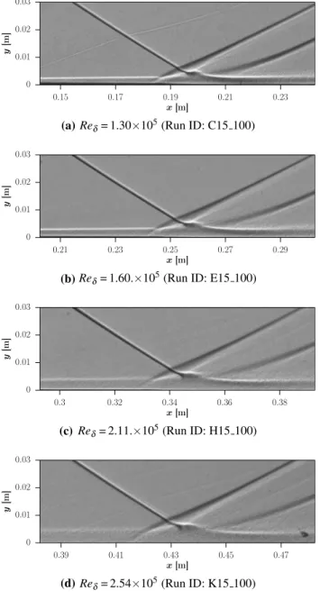
In Fig. 10 shadowgrams of SWBLI are shown with varying Reynolds numbers from Re𝛿=1.30 to 2.54×10⁵ for a constant nominal shock strength 𝜉imp of 2.57. The
figure shows the effect of the boundary layer thickness on the interaction length, because Re𝛿 increases simply by increasing the boundary layer thickness. With increasing Re𝛿 the interaction length L increases, from 22.0 mm in Fig. 10a to 31.9 mm in Fig. 10d (see Table 3).
0 5 10 15 20 0.0 0.5 1.0 1.5 2.0 uSh oc k /U ∞ [%] time [ms] First run Second run d= 18 mm
(a)ξimp= 3.47 & 3.48
0 5 10 15 20 0.0 0.5 1.0 1.5 2.0 uSh oc k /U ∞ [%] time [ms] d= 20 mm (b)ξimp= 3.73 & 3.73 0 5 10 15 20 0.0 0.5 1.0 1.5 2.0 uSh oc k /U ∞ [% ] time [ms] d= 22 mm (c)ξimp= 3.97 & 3.92 0 5 10 15 20 0.0 0.5 1.0 1.5 2.0 uSh oc k /U ∞ [% ] time [ms] d= 24 mm (d)ξimp= 4.14 & 4.16 0 5 10 15 20 0.0 0.5 1.0 1.5 2.0 uSh oc k /U ∞ [% ] time [ms] d= 26 mm (e) ξimp= 4.18 0 5 10 15 20 0.0 0.5 1.0 1.5 2.0 uSh oc k /U ∞ [% ] time [ms] d= 28 mm (f)ξimp= 4.40
Fig. 7 Velocity time histories of the moving impinging shocks at
y=21 mm with increasing normalized shock strengths. From a–d the
measurement reproducibility is shown
Table 1 Boundary layer conditions at varying streamwise positions Experiment x (mm) 𝛿 (mm) 𝛿∗ (mm) 𝜃 (mm) Re1 (m−1) Re 𝛿 (105) cf P0 (bar) T0 (K) Pitot1 153 2.18 0.72 0.14 46.2 1.01 0.00178 5.37 272.9 Pitot2 213 2.99 1.06 0.19 46.0 1.37 0.00160 4.98 260.5 Pitot3 273 3.69 1.30 0.24 46.3 1.71 0.00151 5.02 260.7 Pitot4 333 4.34 1.49 0.28 45.6 1.98 0.00148 5.34 274.3 Pitot5 393 5.07 1.79 0.33 46.2 2.34 0.00141 5.06 262.6
4.3 Modified interaction length scaling
The original scaling approach described by Souverein et al. (2013) accounts for Mach number, shock-strength and bound-ary-layer effects on the interaction length. The interaction length L is defined as the distance between the upstream influ-ence point x1 and the inviscid shock location (impingement point or kink of the ramp). The cited approach describes the scaled interaction length L∗ as a function of the scaled interac-tion strength S∗ , which are defined as:
(1) S∗= kcp= 2k 𝛾 pout pin −1 M2 (2) L∗= L 𝛿∗ sin(𝛽)sin(𝜑) sin(𝛽 − 𝜑)
cp is the pressure coefficient downstream of the reflected
shock and k is chosen to obtain S∗ of approximately 1 at the
onset of separation. k is a constant function (step function) having two pieces only ( k=3 for Re𝜃 ⩽104 and k=2.5 for Re𝜃>104 ). The interaction length L is scaled with the
deflection angle of the shock 𝜑 , the shock angle 𝛽 and the
displacement thickness 𝛿∗.
To verify the scaling approach for a high Reynolds number range, the approved experimental data set of Set-tles et al. (1976) for two-dimensional, stationary SWBLIs induced by a ramp is used in addition to the present data set obtained in the quasi-steady case. By focusing on these two large data sets, physical causes of data scattering such as
−0.04 −0.03 −0.02 −0.01 0.00 0.01 0.02 0.03 0.04 0.34 0.35 0.36 0.37 S R z [ m ] x[m]
Fig. 8 Flow separation topology showing the lateral flow component within the separation bubble. Visualization using the oil film interfer-ometry technique. (Run ID: H15_100)
(a)
(b)
(c)
(d)
Fig. 9 Shadowgrams of SWBLI with increasing impinging shock strength
differences in test facilities, experimental setups or meas-urement techniques, which are not taken into account in the scaling method, could be reduced to a minimum, as will be demonstrated later in this paper.
In Fig. 11a the data by Settles et al. are scaled in accord-ance with the original approach from Souverein et al. (2013). The Reynolds number values are in the range of 5.2×10⁵
≤Re𝛿≤ 7.5×10⁶ ( 2.3×10⁴ ≤Re𝜃 ≤ 3.1×10⁵ ), given by the corresponding colorbar.
In Fig. 11b the results of the present study are scaled according to Souverein et al. (2013), but with a fixed factor k=2.5 in S∗ . The ranges of the scaled interaction strengths is 0.83 ≤S∗ ≤ 4.02 and of the scaled interaction lengths
is 1.28 ≤L∗ ≤ 29.70. The Reynolds number values are in the range of 1.27×10⁵≤Re
𝛿≤ 2.5×10⁵ ( 8.1×10³≤Re𝜃 ≤ 1.7×10⁴ ), indicated by the corresponding colorbar.
In its original form cp has been calculated
consider-ing a plane shock with the oblique shock theory based on the Mach number and the deflection angle 𝜑 at the boundary layer edge. For the impinging non-planar bow shock in the current setup, however, the deflection angle expected at the boundary layer edge differs from the one expected in the plane of the flat plate. Thus, to calculate cp
the deflection angle 𝜑 at the virtual bow shock position at
the flat-plate surface (impingement point) has been used. In accordance with the oblique-shock theory for inviscid (a)
(b)
(d) (c)
Fig. 10 Shadowgrams of SWBLI with increasing Reynolds number
0.0 0.5 1.0 1.5 2.0 2.5 3.0 3.5 4.0 0.0 0.2 0.4 0.6 0.8 1.0 1.2 1.4 L ∗ S∗ Settles et al. 1976 ϕ= 20◦ ϕ= 18◦ ϕ= 16◦ ϕ= 14◦ ϕ= 10◦ 0 1×10⁶ 2×10⁶ 3×10⁶ 4×10⁶ 5×10⁶ 6×10⁶ 7×10⁶ 8×10⁶ Reδ
(a) Data from Settles et al. (1976).
0 5 10 15 20 25 30 35 0.0 1.0 2.0 3.0 4.0 5.0 L ∗ S∗ 1.2×10⁵ 1.4×10⁵ 1.6×10⁵ 1.8×10⁵ 2.0×10⁵ 2.2×10⁵ 2.4×10⁵ 2.6×10⁵ Reδ
(b)Steady shock wave data from the present study. Fig. 11 Scaling according to Souverein et al. (2013): a original approach, b with a fixed factor k=2.5
flow all impinging shock strengths were weak enough to be reflected without a Mach-stem. However, the far-reach-ing results come close to this upper limit for an inviscid shock reflection at 𝛽imp =39.52◦ for M=3 , corresponding to S∗=5 for k=2.5 . The interaction length L is measured
by using shadowgrams as mentioned above.
The high scattering of the measurement values appear-ing in both cases in Fig. 11 for any roughly constant inter-action strength S∗ indicates a clear stratification by the Reynolds number. As mentioned above, the influence of the Reynolds number was nominally considered in the original scaling approach by the step function k. The data presented in Fig. 11 clearly show that a step function is inadequate and only a continuous function can describe the influence of the Reynolds number. Thus, a correction is required.
To improve this, we propose to introduce a new cor-relation function K instead of the step function k, which describes the complex influence of the Reynolds number in the wide range of shock intensities. In order to plausibly eliminate the existing Reynolds-number stratification of the validation data, the heuristic trial-and-error approach was applied to find a suitable form for K. As a result, the fol-lowing form of the correlation has proven to be particularly useful:
The reference Reynolds number Reref must be here in the range of a well-developed turbulent boundary layer, and we have decided to use Reref=2×10⁵ for further analysis. The constants a and b are the appropriate fitting parameters of this correlation to be found. To avoid confusion with the original scaling approach of Souverein et al. (2013), we introduce finally the normalized pressure coefficient c∗
p
=K(Re, cp)×cp instead of S∗ =k×c
p . This results in the modified scaling approach:
with
In contrast to the basic scaling approach, where k plays the role of a critical pressure coefficient corresponding to incipi-ent separation, in the modified approach, the incipiincipi-ent sepa-ration does not play a special role in predicting the size of the interaction length.
Using the method of least squares, we look for the appro-priate parameters a and b in K(Re, cp) in order to
approxi-mate the combined experimental data of Settles et al. (1976) and of the present study in the best possible way. The search (3) K= (Re𝛿∕Reref) a×(cpb) (4) L∗=f(Re𝛿, cp) =f(c∗p) (5) c∗p=K(Re, cp) ×cp= ( Re𝛿 Reref )a×(cp)b ×cp.
revealed the optimal parameter combination with a= −0.27
and b=1.41:
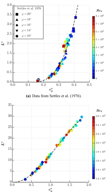
Figure 12a shows the data of Fig. 11a, scaled using the found correlation function K(Re, cp) . The resulting c∗p range yields to
0.13 ≤c∗p ≤ 1.82. By using the modified scaling approach the best-fit approximation found, for the data of Settles et al. (1976) (Fig. 12a, dashed line), is described by the polynomial: In Fig. 12b the data from the present study are shown apply-ing the modified scalapply-ing approach. For these SWBLIs the influence of three-dimensionality cannot be neglected, as shown in the last chapter. Therefore, a different best-fit approximation for the scaled interaction length results, was found in this case (Fig. 12b, dashed line):
The modified scaling approach reduces the data scattering of both data sets significantly. The resulting stratification of the measured values L∗ by the Reynolds number is
negligi-ble in both cases. The best-fit correlation (Eq. 8) describes the experimental data with a coefficient of determination R2
(from 0 to 1) of 0.99.
An alternative representation of the same data is shown in Fig. 13. It explicitly shows the dependence of the interac-tion length L∗ on the Reynolds number Re
𝛿 . In Fig. 13a the data of Settles et al. (1976) for different ramp angles ( cp
values) are presented. The measurement points are shown as symbols. The solid lines shown for five different cp values
from cp = 0.173 to 0.451 ( 𝜑=10◦ to 20◦ in sector 2) were calculated using Eqs. 6 and 7. The good agreement confirms that the Reynolds number influence is adequately reflected in the proposed approach. The data scattering around the lines for each nominal cp value is partly due to a slight decrease
in Mach number along the test section (from sector 1 to 3) reported by Settles et al. (1976), which leads to an increase of the experimental value of cp at constant ramp angle.
Figure 12b shows in a similar way the results of the cur-rent study for a selection of shock intensities. The results obtained using Eqs. 6 and 8 (solid lines) correlate very well with the corresponding experimental data (symbols).
Figure 14a shows a wide range of 2-D SWBLI data from different institutions scaled according to the cited approach of Souverein et al. (2013). All investigations considered are high-lighted in Table 2, with the corresponding symbols. The data collection is largely based on the selection of Souverein et al. (6) c∗p = ( Re𝛿 2×10⁵ )−0.27×(cp)1.41 ×cp (7) L∗= −3.4× (c∗p)2+142.33× (c∗p)4. (8) L∗= −1.14×c∗p+19.16× (c∗p)2−5.36× (c∗ p) 3.
(2013). However, only part of these data was used in the present plot because the authors do not know all the required parameters in each of the original data sets. In this presentation, the cur-rent data (“+” symbol) seem to continue the trend of the data from the literature well. The scattering of the current data due to the Reynolds number variation does not seem to be particularly noticeable compared to the scattering of the remaining data.
Figure 14b shows the same data again using the proposed modified scaling approach according to Eq. 6. It is remarkable that although this scaling approach leads to a significant reduc-tion of the scatter within each individual data set, the com-mon course of the data breaks up into at least two individual courses. On the one hand, the data describing the incident shock
interaction (see Table 2) remain together very well, thus con-firming the trend found in the current data. On the other hand, the data obtained at compression ramps form another group that looks less homogeneous but still follows its own trend. Additional parameter effects seem to appear which might have been hidden before inside the scattering, such as wall tempera-ture effects, effects from fences and more. It can be concluded that the modified scaling approach provides a reliable basis for the representation of the own stationary data of incident shock interactions. On this basis, the effect of the moving shock fronts on the extent of the interaction area can be analyzed well in a further step. 0.0 0.5 1.0 1.5 2.0 2.5 3.0 3.5 4.0 0.0 0.1 0.2 0.3 0.4 0.5 L ∗ c∗ p Settles et al. 1976 ϕ= 20◦ ϕ= 18◦ ϕ= 16◦ ϕ= 14◦ ϕ= 10◦ 0 1×10⁶ 2×10⁶ 3×10⁶ 4×10⁶ 5×10⁶ 6×10⁶ 7×10⁶ 8×10⁶ Reδ
(a)Data from Settles et al. (1976).
0 5 10 15 20 25 30 35 0.0 0.5 1.0 1.5 2.0 L ∗ c∗ p 1.2×10⁵ 1.4×10⁵ 1.6×10⁵ 1.8×10⁵ 2.0×10⁵ 2.2×10⁵ 2.4×10⁵ 2.6×10⁵ Reδ
(b)Steady shock wave data from the present study. Fig. 12 Scaling based on the modified approach (Eq. 6). Lines are corresponding best-fit approximations (Eqs. 7 and 8)
0.0 0.5 1.0 1.5 2.0 2.5 3.0 3.5 4.0 105 106 107 0.0 0.5 1.0 1.5 2.0 2.5 3.0 3.5 4.0 105 106 107 L ∗ Reδ Settles et al. 1976 Sector 1 Sector 2 Sector 3 cp= 0.451 cp= 0.386 cp= 0.326 cp= 0.270 cp= 0.173
(a)Data from Settles et al. (1976).
0 5 10 15 20 25 30 35 40 105 5×10⁵ L ∗ Reδ
present data (steady) cp= 1.536 cp= 1.232 cp= 0.920 cp= 0.728 cp= 0.612 cp= 0.504 cp= 0.332
(b)Steady shock wave data from the present study. Fig. 13 Reynolds number influence on the scaled interaction length. Validation of the modified scaling method
4.4 Influence of a moving impinging shock on SWBLI
In this chapter, the influence of a uniformly moving imping-ing shock on the shock-wave/boundary-layer interaction flow is analyzed. The turbulent boundary layer on the flat plate develops as in the stationary measurements. The traveling SWBLI on the flat plate was induced by a movable, cylin-drical shock generator. The impinging shock front moving upstream induces in all cases a separation bubble on the plate which follows the shock front movement. In the present study, a traveling Mach number of Mtrav≈ 0.5 was investigated.
For each interaction strength, a shadowgram taken before the shock generator launch is shown on the left-hand side of
Fig. 15, and a shadowgram taken during the uniform traveling speed is shown on its right hand side. The impinging shock angle (thus, the local shock strength) changes with the shock generator velocity. Because the shock-wave Mach number changes from
Ms=3 to Ms=M∞ + Mtrav≈ 3.5, the impinging shock angle decreases although the impinging shock strength increases. The interaction length L of the moving SWBLI, is for all cases smaller than the one of the stationary interaction. This is partly due to the thinning of the boundary layer with decreasing x-coordinate, and partly due to stronger compressibility effects in the interaction zone (higher Mach number). In Table 4 the quantitative results for each pair of shadowgrams shown in Fig. 15, evaluated as described in Sect. 4.3, are presented.
Table 2 Data collection considered in Fig. 14
a
NASA-Ames Research Center b
University of Princeton
c
University of Illinois
dDelft University of Technology e
Institut Universitaire des Systémes Thermiques Industriels, Marseille
Institute Literature Re𝛿 M Symbol
Compression ramps
NAa Thomke and Roshko (1969) 1.87–7.88×10⁶ 3≤
M≤5 ⋄ UPb,1 Settles et al. (1976) 0.52–7.54×10⁶ 2.9 × UPb,2 Dolling and Or (1985) 1.43×10⁶ 2.9 □ UPb,2 Selig et al. (1989) 1.69×10⁶ 2.9 □ UIc Kuntz et al. (1987) 0.31×10⁶ 2.9 ◦
Incident shock reflection
TUDd Humble (2009) 0.61×10⁶ 2.1 ▿ IUSTIe Piponniau (2009) 5.3×10⁶ 2.3 ▿ IUSTIe Souverein (2010) 0.06–0.62×10⁶ 2.3 ▿ Present study 0.12–0.26×10⁶ 3 + 0 5 10 15 20 25 30 35 0.0 1.0 2.0 3.0 4.0 5.0 L ∗ S∗
(a)Original scaling approach.
0 5 10 15 20 25 30 35 0.0 0.5 1.0 1.5 2.0 L ∗ c∗ p (b)Modified scaling approach. Fig. 14 Scaling of the interaction length, with symbols as in Table 2
The dynamic shock boundary layer interactions for upstream moving impinging shocks with a traveling Mach number of Mtrav ≈ 0.5 can be quantitatively compared to the stationary
interac-tions by using the modified scaling law proposed in previous chapters. In Fig. 16 the results obtained at the state before the shock generator launch are shown as green dots. The reference data used to obtain the modified scaling law in Sect. 4.3 are shown additionally as black dots. The green and the black dots together describe the stationary situation and show as expected very good agreement. The difference in span of the cylinder models (245/200 mm), is thus negligible for the scaled results.
The results of the uniformly moving interactions are shown by red dots following the same trend line as the sta-tionary results. The best-fit correlation (Eq. 8) describes these
experimental data with a coefficient of determination R2 of 0.93
with a maximum deviation of 𝛥L∗=1.8 . Thus, the scattering of data is higher in this case but still comparable to the scat-tering of the stationary interactions with values of R2=0.99
and a maximum deviation of 𝛥L∗=0.8 . The reproducibility
of the scaling results has been analyzed with four shock gen-erators. The discrepancy of the non-dimensional interaction length L∗ for the three shock generators with diameters d of
18 mm, 20 mm and 22 mm, which were used twice, is below 𝛥L∗ = 1.25. A higher discrepancy exists for the shock generator with d = 24 mm only, between the experiment and the rerun, of 𝛥L∗ = 2.5. Therefore, it can be stated that in the investigated
shock speed range (up to ≈ 15% freestream velocity) the scaled interaction length can be predicted by the scaling law found for Fig. 15 Shadowgrams of quasi-steady (left) and moving (right) SWBLI using the movable shock generators
stationary SWBLIs. Thus, the resulting non-dimensional inter-action length is dependent on the displacement thickness of the boundary layer, the impinging shock strength and the impinging shock angle resulting from the shock-wave Mach number Ms.
5 Conclusion
The scalability of the interactions induced by impinging shock waves traveling over the turbulent boundary layer with nearly constant shock strengths has been experimen-tally studied using the shadowgraph technique. In a broad-based study, stationary reference SWBLIs were examined to evaluate the effect of shock movement. The most significant findings of the study may be summarized as follows: 1. A special experimental setup was developed to
inves-tigate the static and dynamic SWBLI under similar conditions. The impinging shock fronts induced a flow separation on the flat plate in all investigated cases. The resulting flow is strictly speaking not two-dimensional, because the separation line has an arc-like shape and the reverse flow contained a lateral flow component. Another aspect was that the SWBLIs were so strong that they were outside the limits of known scaling laws. Therefore, a special scaling law as a reference for the considerations of traveling SWBLI was needed. 2. A modified scaling approach for the interaction length L
was proposed, which is based on the method described by Souverein et al. (2013). This modification consid-ering the Reynolds number impact was successfully validated with the data available for two-dimensional,
steady SWBLI from the literature and own data from the present study. Using this method the corresponding correlation function K(Re, cp) could be determined.
3. By applying the enhanced scaling approach, a significant reduction in data scatter could be observed for all available data sets compared to the original approach. Due to this improvement, it was immediately apparent that the common course of the data actually breaks up into at least two indi-vidual progressions. One formed for incident shock interac-tions and the other formed for data obtained at compression ramps that is less homogeneous. Due to the lower scattering, additional parameter effects seem to appear which might have been hidden before (temperature effects, etc.). 4. Available data from incident shock interactions were
shown to be in very good agreement with data obtained in the present work. These data coincided to a very reli-able and systematic dependence, which could be well approximated applying scaling law in the entire shock intensity range investigated. The resulting very low scat-ter of the stationary reference SWBLIs was a crucial prerequisite for the analysis of the influence of a moving impinging shock.
5. This reference scaling law was used to analyze the impact of the moving impinging shocks on the non-dimensional interaction lengths. The results obtained with moving shock fronts were within the scattering range of the ref-erence steady-state data, but only if the true shock wave Mach number of 3.5 was taken into account. It can be concluded, that below the investigated traveling speed of
≈ 15% freestream velocity the interaction length of the
traveling SWBLI can be predicted by applying the found scaling law, valid for stationary flows.
Acknowledgements Open Access funding provided by Projekt DEAL. The authors gratefully acknowledge the support by the anonymous reviewers of this manuscript.
Open Access This article is licensed under a Creative Commons Attri-bution 4.0 International License, which permits use, sharing, adapta-tion, distribution and reproduction in any medium or format, as long as you give appropriate credit to the original author(s) and the source, provide a link to the Creative Commons licence, and indicate if changes were made. The images or other third party material in this article are included in the article’s Creative Commons licence, unless indicated otherwise in a credit line to the material. If material is not included in the article’s Creative Commons licence and your intended use is not permitted by statutory regulation or exceeds the permitted use, you will need to obtain permission directly from the copyright holder. To view a copy of this licence, visit http://creat iveco mmons .org/licen ses/by/4.0/.
Appendix
See Tables 3, 4. 0 5 10 15 20 25 30 35 0.0 0.5 1.0 1.5 2.0 0 5 10 15 20 25 30 35 0.0 0.5 1.0 1.5 2.0 L ∗ c∗ p L ∗ c∗ p present data (steady) MS,move= 0MS,move= 0.5
Fig. 16 Influence of the traveling impinging shock fronts, listed in Table 4, on the interaction length scaled using the modified approach adjusted for steady flows (see Eq. 6)
Table 3 Tes t matr ix of t he s tationar y shado wg ram anal ysis 𝜉imp cp Run ID d (mm) 𝛥 x (mm) 𝛥 y (mm) P0 (bar) T0 (K) R e1 (10 6) 𝛿 (mm) 𝛿 ∗ (mm) ximp (mm) 𝛽imp ( ◦) c ∗ p L (mm) L ∗ 1.821 0.332 D5_80 5 84 80 5.03 264.4 45.41 2.88 1.00 208.4 25.8 0.340 6.2 1.28 1.821 0.332 F5_80 5 144 80 5.03 258.7 46.97 3.60 1.25 268.2 25.8 0.335 8.9 1.45 1.821 0.332 H5_80 5 204 80 4.99 263.4 45.31 4.33 1.52 329.4 25.8 0.332 10.1 1.38 1.821 0.332 J5_80 5 264 80 4.99 259.9 46.28 5.03 1.77 388.9 25.8 0.329 11.2 1.30 2.157 0.504 C10_100 10 64 100 5.03 258.5 47.07 2.70 0.93 192.8 28.1 0.528 13.5 4.28 2.157 0.504 D10_100 10 94 100 5.05 263.7 45.75 3.06 1.06 222.7 28.1 0.523 14.0 3.90 2.157 0.504 F10_100 10 154 100 5.04 261.2 46.34 3.78 1.32 283.5 28.1 0.511 16.6 3.72 2.157 0.504 H10_100 10 214 100 5.02 265.1 45.10 4.50 1.58 343.7 28.1 0.503 19.1 3.56 2.157 0.504 J10_100 10 274 100 5.02 259.6 46.61 5.21 1.83 403.7 28.1 0.494 20.8 3.33 2.359 0.612 E10_80 10 124 80 4.98 262.9 45.38 2.98 1.03 216.8 29.4 0.645 18.2 6.14 2.359 0.612 G10_80 10 184 80 5.04 260.8 46.52 3.70 1.29 276.8 29.4 0.625 19.2 5.17 2.359 0.612 I10_80 10 244 80 4.99 262.0 45.73 4.42 1.55 337.0 29.4 0.611 22.3 5.00 2.359 0.612 K10_80 10 304 80 5.01 260.5 46.32 5.12 1.80 396.5 29.4 0.598 24.8 4.78 2.565 0.728 C15_100 15 99 100 5.04 261.3 46.34 2.81 0.97 202.5 30.7 0.784 22.0 9.07 2.565 0.728 D15_100 15 129 100 5.30 272.4 45.73 3.16 1.09 231.3 30.7 0.770 22.2 8.12 2.565 0.728 E15_100 15 159 100 5.03 264.3 45.44 3.53 1.23 262.6 30.7 0.756 24.5 8.01 2.565 0.728 F15_100 15 189 100 4.88 261.4 44.86 3.88 1.36 292.3 30.7 0.746 27.8 8.23 2.565 0.728 G15_100 15 219 100 5.06 266.5 45.15 4.24 1.48 322.2 30.7 0.734 28.3 7.65 2.565 0.728 H15_100 15 249 100 5.04 263.4 45.82 4.60 1.62 352.8 30.7 0.721 27.7 6.88 2.565 0.728 I15_100 15 279 100 5.33 274.2 45.52 4.95 1.74 382.0 30.7 0.713 30.9 7.10 2.565 0.728 J15_100 15 309 100 4.90 255.9 46.55 5.31 1.87 412.5 30.7 0.702 31.5 6.74 2.565 0.728 K15_100 15 339 100 5.03 266.9 44.75 5.67 2.00 442.3 30.7 0.699 31.9 6.40 2.890 0.920 F15_80 15 189 80 5.03 258.8 46.95 3.50 1.22 259.9 32.7 0.965 29.3 11.63 2.890 0.920 G15_80 15 219 80 4.88 257.7 45.84 3.83 1.34 287.7 32.7 0.949 30.5 11.03 2.890 0.920 H15_80 15 249 80 5.05 263.2 45.93 4.21 1.47 319.9 32.7 0.927 34.2 11.19 2.890 0.920 I15_80 15 279 80 5.07 263.9 45.93 4.57 1.60 349.7 32.7 0.910 37.3 11.25 2.890 0.920 J15_80 15 309 80 5.30 272.7 45.65 4.93 1.73 379.8 32.7 0.895 37.2 10.37 2.890 0.920 K15_80 15 339 80 4.99 260.3 46.15 5.28 1.86 409.7 32.7 0.877 35.1 9.10 2.960 0.964 F20_100 20 189 100 5.02 264.6 45.32 3.65 1.27 273.1 33.1 1.012 33.0 12.95 2.960 0.964 G20_100 20 219 100 5.23 266.3 46.72 4.01 1.40 302.7 33.1 0.980 34.1 12.17 2.960 0.964 H20_100 20 249 100 5.05 264.3 45.63 4.36 1.53 332.6 33.1 0.965 38.6 12.62 2.960 0.964 I20_100 20 279 100 5.34 273.1 45.89 4.72 1.66 362.6 33.1 0.944 38.3 11.55 2.960 0.964 J20_100 20 309 100 5.10 268.0 45.12 5.08 1.79 392.9 33.1 0.931 40.4 11.30 3.367 1.232 F25_100 25 189 100 5.06 265.7 45.37 3.47 1.21 257.5 35.5 1.344 40.6 20.11 3.367 1.232 G25_100 25 219 100 5.15 265.7 46.17 3.82 1.33 287.1 35.5 1.289 44.1 19.73 3.367 1.232 H25_100 25 249 100 5.10 265.2 45.84 4.18 1.46 317.0 35.5 1.252 44.8 18.30
Table 3 (continued) 𝜉imp cp Run ID d (mm) 𝛥 x (mm) 𝛥 y (mm) P0 (bar) T0 (K) R e1 (10 6) 𝛿 (mm) 𝛿 ∗ (mm) ximp (mm) 𝛽imp ( ◦ ) c ∗ p L (mm) L ∗ 3.367 1.232 I25_100 25 279 100 5.04 266.3 45.03 4.53 1.59 346.9 35.5 1.223 44.8 16.83 3.367 1.232 J25_100 25 309 100 5.22 271.7 45.22 4.89 1.72 377.0 35.5 1.188 48.4 16.81 3.374 1.236 G20_80 20 219 80 4.99 261.8 45.81 3.66 1.28 273.8 35.5 1.317 40.5 18.99 3.374 1.236 H20_80 20 249 80 5.22 267.3 46.36 4.03 1.41 304.2 35.5 1.268 44.9 19.10 3.374 1.236 I20_80 20 279 80 5.08 268.8 44.74 4.39 1.54 334.5 35.5 1.245 43.9 17.09 3.374 1.236 K20_80 20 339 80 5.04 260.9 46.46 5.09 1.79 394.0 35.5 1.163 50.4 16.84 3.764 1.536 F30_100 30 189 100 5.03 265.3 45.19 3.31 1.15 244.2 37.7 1.773 47.1 28.09 3.764 1.536 G30_100 30 219 100 4.97 259.9 46.08 3.66 1.28 273.8 37.7 1.670 48.0 25.73 3.764 1.536 H30_100 30 249 100 5.11 265.6 45.83 4.03 1.41 304.4 37.7 1.598 51.5 25.04 3.764 1.536 I30_100 30 279 100 5.15 267.3 45.73 4.39 1.54 334.9 37.7 1.533 53.1 23.61 3.764 1.536 J30_100 30 309 100 5.35 272.5 46.12 4.74 1.67 364.6 37.7 1.469 55.3 22.72 3.764 1.536 K30_100 30 339 100 5.25 268.4 46.34 5.10 1.80 394.7 37.7 1.414 56.4 21.52 3.842 1.608 G25_80 25 219 80 4.89 259.6 45.44 3.51 1.22 260.9 38.2 1.812 51.7 29.70 3.842 1.608 H25_80 25 249 80 4.96 257.5 46.68 3.87 1.35 290.9 38.2 1.697 53.2 27.62 3.842 1.608 I25_80 25 279 80 5.22 270.4 45.56 4.22 1.48 320.9 38.2 1.641 54.9 26.05 3.842 1.608 J25_80 25 309 80 5.04 259.5 46.87 4.60 1.62 352.6 38.2 1.545 54.3 23.60 3.842 1.608 K25_80 25 339 80 5.07 262.3 46.36 4.93 1.74 380.6 38.2 1.498 58.1 23.47 Shoc k g ener at or widt h = 245 mm
References
Adler A, Hauberg S (2019) The canny-algorithm source code. Retrieved July 15, 2019. https ://sourc eforg e.net/p/octav e/image /ci/relea se-2.4.1/tree/inst/edge.m
Babinsky H, Harvey JK (2011) Shock wave–boundary-layer interac-tions. Cambridge University Press, Cambridge
Bruce P, Babinsky H (2008) Unsteady shock wave dynamics. J Fluid Mech 603:463–473
Canny J (1987) A computational approach to edge detection. In: Read-ings in computer vision. Elsevier, pp 184–203
Chapman GT, Tobak M (1988) Bifurcations in unsteady aerodynamics-implications for testing. NASA TM 100083
Chapman DR, Kuehn DM, Larson HK (1958) Investigation of sepa-rated flows in supersonic and subsonic streams with emphasis on the effect of transition. NACA TN 3869
Clemens NT, Narayanaswamy V (2014) Low-frequency unsteadiness of shock wave/turbulent boundary layer interactions. Annu Rev Fluid Mech 46:469–492
Coon MD, Chapman GT (1995) Experimental study of flow separation on an oscillating flap at mach 2.4. AIAA J 33(2):282–288 Dolling D (1988) Unsteady shock-induced turbulent separation in
Mach 5 cylinder interactions. In: 26th Aerospace sciences meet-ing, p 305
Dolling DS, Or CT (1985) Unsteadiness of the shock wave structure in attached and separated compression ramp flows. Exp Fluids 3(1):24–32
Dupont P, Haddad C, Debieve J (2006) Space and time organiza-tion in a shock-induced separated boundary layer. J Fluid Mech 559:255–277
Elfstrom G (1972) Turbulent hypersonic flow at a wedge-compres-sion corner. J Fluid Mech 53(1):113–127
Gaitonde DV (2015) Progress in shock wave/boundary layer interac-tions. Prog Aerosp Sci 72:80–99
Holden M (1977) Shock wave-turbulent boundary layer interaction in hypersonic flow. In: 15th Aerospace sciences meeting, p 45 Huang P, Bradshaw P, Coakley T (1993) Skin friction and velocity
profile family for compressible turbulent boundary layers. AIAA J 31(9):1600–1604
Humble RA (2009) Unsteady flow organization of a shock wave/bound-ary-layer interaction. Ph.D. thesis, Delft University of Technology Kuntz DW, Amatucci VA, Addy AL (1987) Turbulent boundary-layer properties downstream of the shock-wave/boundary-layer interac-tion. AIAA J 25(5):668–675
Liu K, Zhang K (2011) Experiment of dynamic angle-of-attack on a side wall compression scramjet inlet at Mach 3.85. In: 17th AIAA international space planes and hypersonic systems and technologies conference, AIAA 2011-2348
Moeckel WE (1949) Approximate method for predicting form and location of detached shock waves ahead of plane or axially sym-metric bodies. NACA TN 1921
Muck K, Bogdonoff S, Dussauge JP (1985) Structure of the wall pressure fluctuations in a shock-induced separated turbulent flow. In: 23rd aerospace sciences meeting, p 179
Park SO, Chung Y, Sung HJ (1994) Numerical study of unsteady supersonic compression ramp flows. AIAA J 32(1):216–218 Park SO, Lee C, Kang K (2001) Navier–Stokes analysis of a
super-sonic flow over moving compression ramp. In: 39th Aerospace sciences meeting and exhibit, p 568
Pasquariello V, Hickel S, Adams N, Hammerl G, Wall W, Daub D, Willems S, Gülhan A (2015) Coupled simulation of shock-wave/ turbulent boundary-layer interaction over a flexible panel. In: 6th European conference for aerospace sciences
Table 4 Test matrix for the SWBLIs with a uniform traveling speed Mtrav , see Fig. 15
Shock generator width = 200 mm
𝜉imp cp Run ID d (mm) 𝛥y (mm) P0 (bar) T0 (K) Re1 (106) Ms 𝛿 (mm) 𝛿∗ (mm) ximp (mm) 𝛽imp ( ◦) c∗p L (mm) L ∗ 3.14 1.080 1.steady18 18 80 4.58 244.4 46.74 3 4.99 1.76 385.4 34.1 1.032 43.0 13.31 3.47 0.996 1.move18 18 80 4.58 244.4 46.74 3.46 4.35 1.52 331.2 30.7 0.992 31.6 12.19 3.15 1.084 2.steady18 18 80 4.70 250.9 46.05 3 4.99 1.75 384.8 34.2 1.040 40.4 12.57 3.48 0.990 2.move18 18 80 4.70 250.9 46.05 3.47 4.27 1.50 325.1 30.6 0.995 31.3 12.23 3.32 1.199 1.steady20 20 80 4.58 244.8 46.61 3 5.11 1.80 395.6 35.2 1.128 45.7 14.87 3.73 1.113 1.move20 20 80 4.58 244.8 46.61 3.47 4.53 1.59 347.0 31.8 1.094 35.8 14.39 3.31 1.191 2.steady20 20 80 4.71 251.6 45.89 3 5.12 1.80 396.1 35.1 1.127 46.9 15.19 3.73 1.104 2.move20 20 80 4.71 251.6 45.89 3.48 4.44 1.56 339.4 31.7 1.097 35.8 14.57 3.49 1.319 1.steady22 22 80 4.52 245.9 45.72 3 5.15 1.81 398.3 36.2 1.237 49.5 17.07 3.97 1.228 1.move22 22 80 4.52 245.9 45.72 3.48 4.54 1.59 347.7 32.8 1.212 42.2 18.18 3.49 1.320 2.steady22 22 80 4.70 249.6 46.37 3 5.15 1.81 398.8 36.2 1.230 53.0 18.28 3.92 1.212 2.move22 22 80 4.70 249.6 46.37 3.47 4.45 1.56 339.9 32.6 1.199 40.8 17.79 3.65 1.440 1.steady24 24 80 4.53 248.2 45.07 3 5.18 1.82 401.2 37.1 1.343 56.6 20.49 4.14 1.342 1.move24 24 80 4.53 248.2 45.07 3.46 4.49 1.57 343.0 33.7 1.336 44.8 20.77 3.66 1.453 2.steady24 24 80 4.59 249.9 45.26 3 5.17 1.82 400.5 37.2 1.352 52.0 18.96 4.16 1.342 2.move24 24 80 4.59 249.9 45.26 3.47 4.53 1.59 346.5 33.7 1.329 39.7 18.27 3.83 1.600 1.steady26 26 80 4.68 249.0 46.38 3 5.22 1.84 404.5 38.1 1.448 58.9 22.41 4.18 1.391 1.move26 26 80 4.68 249.0 46.38 3.44 4.54 1.59 347.2 34.1 1.361 47.2 22.23 3.99 1.771 1.steady28 28 80 4.65 249.2 46.03 3 5.26 1.85 407.6 39.0 1.578 57.6 22.75 4.40 1.488 1.move28 28 80 4.65 249.2 46.03 3.46 4.43 1.55 338.1 34.9 1.475 48.6 24.52
Piponniau S (2009) Instationnarités dans les décollements compressi-bles: cas des couches limites soumises à ondes de choc. Ph.D. thesis, Université de Provence
Poggie J, Smits A (2001) Shock unsteadiness in a reattaching shear layer. J Fluid Mech 429:155–185
Roberts TP (1989) Dynamic effects of hypersonic separated flow. Ph.D. thesis, University of Southampton
Schülein E (2006) Skin friction and heat flux measurements in shock/ boundary layer interaction flows. AIAA J 44(8):1732–1741 Schülein E, Wagner A (2015) Freestream disturbance characterization
in DNW-RWG at Mach 3 and 6. DLR 224 2014 C 169
Schülein E, Krogmann P, Stanewsky E (1996) Documentation of two-dimensional impinging shock/turbulent boundary layer interaction flow. DLR Report DLR IB 223-96 A 49
Selig MS, Andreopoulos J, Muck KC, Dussauge JP, Smits AJ (1989) Turbulence structure in a shock wave/turbulent boundary-layer interaction. AIAA J 27(7):862–869
Settles GS, Bogdonoff SM, Vas IE (1976) Incipient separation of a supersonic turbulent boundary layer at high Reynolds numbers. AIAA J 14(1):50–56
Settles GS, Perkins J, Bogdonoff S (1981) Upstream influence scal-ing of 2d and 3d shock/turbulent boundary layer interactions at compression corners. In: 19th aerospace sciences meeting, p 334
Souverein LJ (2010) On the scaling and unsteadiness of shock induced separation. Ph.D. thesis, Delft University of Technology Souverein L, Bakker P, Dupont P (2013) A scaling analysis for
tur-bulent shock-wave/boundary-layer interactions. J Fluid Mech 714:505–535
Thomke G, Roshko A (1969) Incipient separation of a turbulent bound-ary layer at high Reynolds number in two-dimensional supersonic flow over a compression corner. NASA CR 73308
Zheltovodov A, Schülein E, Horstman C (1993) Development of separation in the region where a shock interacts with a turbulent boundary layer perturbed by rarefaction waves. J Appl Mech Tech Phys 34(3):346–354
Zukoski EE (1967) Turbulent boundary-layer separation in front of a forward-facing step. AIAA J 5(10):1746–1753
Publisher’s Note Springer Nature remains neutral with regard to jurisdictional claims in published maps and institutional affiliations.