Demographic Trends, Fiscal Policy and Trade De
fi
cits
Andrea Ferrero
∗New York University
JOB MARKET PAPER
December 13, 2005
Abstract
In this paper, I argue that demographic factors play a central role in accounting for the trade deficit experienced by the U.S. during the last three decades. The main idea is that cross-country demographic differentials lead to adjustments in savings and investments which are associated with international capitalflows towards relatively young and rapidly growing economies. I develop a tractable two-country framework with life-cycle structure that formalizes this intuition. The model permits to illustrate analytically and quanti-tatively the contribution of demographic variables in determining the equilibrium trade balance. I show that persistent differences in population aging can explain a significant fraction of the negative trend in the U.S. trade balance. Notably, the explicit consid-eration of the demographic transition also helps to reconcile the dynamics of the trade balance with the evolution of the U.S.fiscal deficits and generates a declining pattern for the real interest rate broadly consistent with the data.
∗I would like to express my gratitude to David Backus, Pierpaolo Benigno and especially Mark Gertler for
their advice and guidance throughout this project. I have also benefited from comments by Jonathan Eaton, Jesus Fernandez-Villaverde, John Leahy, Sydney Ludvigson, Fabrizio Perri, Thomas Sargent and Martin Schneider as well as from other seminar participants at NYU. All errors remain my own responsibility. Department of Economics - 110 Fifth Avenue, 5thfloor - New York, NY 10011.
1
Introduction and Related Literature
The dynamics of the U.S. external position have recently received a great deal of attention in the economic community. In 2004 the U.S. trade balance reached a record deficit of more than 5% of GDP. This figure is the result of a long run trend that is projected to continue, at least in the near future.
The objective of this paper is to highlight the central role played by demographic factors in explaining the U.S. trade deficit during the last three decades. The results of this work demonstrate that demographic differentials are crucial to:
1. Account for the negatively sloped trend of the U.S. trade balance.
2. Reconcile the dynamics of the trade balance with the evolution offiscal deficits. 3. Capture the persistent decline of the world real interest rate.
The key driving force behind these findings is the adjustment of private savings to the demographic transition. In an economy with aging population, individuals plan for longer retirement periods by saving more during their working years. Moreover, during retirement, their consumption is spread over a longer period of time. If the economy is open and de-mographic profiles differ across countries, relative savings generate capital flows that are associated with variations in the stock of net foreign assets and trade imbalances.
For the purpose of this paper, I concentrate on the bilateral trade balance between the United States and the other six major industrialized countries of the world economy (Canada, France, Germany, Italy, Japan and the United Kingdom - henceforth, the G6). The reason for narrowing the focus on this subset of the U.S. trade partners is that the G6 feature an economic structure that is highly comparable to the U.S. under several respects. At the same time, however, the G6 display notable differences in terms of demographic variables, as I illustrate more thoroughly in the next section.
The left panel of Figure 1 shows that, at least until the late 1990s, the U.S. trade balance vis-a-vis the G6 accounted for the bulk (about 80% on average) of the total U.S. external imbalance.1 The right panel of Figure 1 depicts the U.S. trade balance against the G6 together
1The recent departure of the U.S. trade balance series vis-a-vis the rest of the world from the series
vis-a-vis the G6 depends upon the capital flows towards the U.S. from oil producers, newly developed and emerging market economies. This aspect of the U.S. external position (the “global saving glut”, in the words of Bernanke [2005]) is not the focus of this paper. See Caballero, Fahri and Gourinchas [2005] for an explanation of this phenomenon based on the inability of emerging market economies to generate enough reliable saving instruments after the Asian crises of the late 1990s.
1960 1968 1976 1984 1992 2000 -6 -5 -4 -3 -2 -1 0 1 YEARS T R A D E B A L A N C E % O F G D P
U.S. TRADE BALANCE (TOTAL and vs. G6)
vs. G6
vs. REST OF THE WORLD
1960 1968 1976 1984 1992 2000 -2.5 -2 -1.5 -1 -0.5 0 0.5 1 YEARS T R A D E B A L A N C E % O F G D P
U.S. TRADE BALANCE vs. G6 (DATA AND TREND)
vs. G6 (DATA) vs. G6 (TREND)
Figure 1: the u.s. trade balance.
with its long run trend. The picture clearly identifies the overall decline of the long run trend and the negative sign which characterizes large part of the sample.
Recent contributions (Caballero, Fahri and Gourinchas [2005] and Engel and Rogers [2005]) have emphasized the role of productivity growth differentials in explaining the U.S. external deficits. An explanation of the dynamics of the U.S. trade deficit based on productivity differentials requires not only current productivity growth to be higher in the U.S. than in the rest of the world but also the expectations of future productivity differentials to be positive and increasing. In the words of Engel and Rogers [2005], “the assumptions on future growth in U.S. shares [of world GDP]that can explain the level in 2004 would imply that the U.S. deficit should have been even larger in earlier years”. Caballero, Fahri and Gourinchas [2005] resolve this issue by postulating permanent growth rate differentials between the U.S. and the G6. The data, however, hardly support this assumption. Figure 2 plots different measures of GDP growth rates for the U.S. and the G6 during the last twenty five years. While differences exist in various periods of the sample, and in some cases persist for few years, the hypothesis of permanent differences appears to be quite extreme.2
This work proposes an alternative explanation for the long run trend of the U.S.
exter-2Productivity growth rate differentials likely play a prominent role in accounting for the variations in the
1980 1984 1988 1992 1996 2000 2004 -3 -2 -1 0 1 2 3 4 5 6 7 YEARS % G D P G R O W T H R A T E PER-CAPITA GDP US (MEAN=1.94%) G6 (MEAN=1.71%) 1980 1984 1988 1992 1996 2000 2004 -1.5 -1 -0.5 0 0.5 1 1.5 2 2.5 3 3.5 YEARS % G D P G R O W T H R A T E PER-WORKER GDP US (MEAN=1.61%) G6 (MEAN=1.50%)
Figure 2: gdp growth rates.
nal position based on demographic factors. The methodological contribution of the paper is to develop a tractable open economy model with life-cycle structure that identifies the transmission mechanism and the quantitative importance of demographic variables for the determination of the equilibrium trade balance. The resulting framework shares the basic features of the neoclassical growth model. The only complication of considering life-cycle behavior and non-stationary demographics derives from the presence of two extra state vari-ables that capture the distribution of wealth across cohorts and the ratio between the number of retirees and the number of workers.
The demographic structure assumed in this paper builds upon the formulation in Blanchard [1985] and Weil [1989] by adding a random transition from employment to retirement, an element of the life-cycle not present in those two studies. In Blanchard [1985], individuals face uncertainty about their lifetime horizon but the survival probability also governs the fertility rate. Hence, an increase in life expectancy also implies an increase in population growth so that the aggregate size of population is constant. On the other hand, in Weil [1989], households are infinitely lived but in each period a new cohort is born so that population grows over time. In this paper, the probability of surviving is decoupled from the population growth rate. It is then possible to isolate the contribution of smaller population growth rates and longer lifetime horizons in determining the equilibrium trade balance. The life-cycle transition
from the labor force into retirement generates a reasonable pattern for aggregate savings in response to demographic shocks. Saving differentials across countries indeed constitute the main driving force behind the adjustment.
The explicit link between demographics and external imbalances has been previously ex-plored in the literature. Obstfeld and Rogoff [1996] discuss some of the basic issues in the context of a two-period life-cycle model. The main prediction of such a framework is that countries with higher population growth rates should display, ceteris paribus, higher saving rates. The two-period model necessarily treats the lifetime horizon as fixed (and known). This paper instead emphasizes the importance of variable life expectancy in shaping the in-dividual consumption-savings decisions. Countries where inin-dividuals live on average longer are associated with higher savings rates. Since those countries also feature lower population growth rates, the results in this paper are largely consistent with the data and reverse the argument in the traditional life-cycle literature.3
The quantitative importance of cross-country demographic differentials on the trade balance has recently been stressed by Henriksen [2002] and Feroli [2003] in the context of an open economy computable overlapping generation (OLG) model.4 Domeij and Fl´oden [2004] also simulate an open economy OLG framework driven by demographic differentials and test the explanatory power of the data artificially generated by the calibrated model for the time series of the U.S. current account. Their findings are consistent with a significant effect of demographic variables on external imbalances. The model in this paper remains considerably more tractable than a standard OLG framework. Yet, it provides a framework that can be employed to perform a number of numerical experiments. After illustrating analytically how demographic factors impact the trade balance, I present a quantitative analysis that shows how demographic forces are crucial to account for the declining trend in the U.S. trade balance in the last three decades.
The one source of short run variation that I consider in this paper is fiscal policy. In the absence of voluntary bequests, the presence of life-cycle features breaks one of the assumptions at the core of Ricardian equivalence. Therefore, I can study the impact of fiscal policy on the trade balance in an environment with time-varying demographic differentials across countries. Fiscal deficits alone lead to modest trade deficits, as also recently suggested by
3
Brooks [2003] considers a four-period multiregion overlapping generation model and shows that the current demographic structure should be associated with capitalflows from the G7 towards developing countries. This result also depends crucially on thefixed lifetime horizon assumed in that paper.
Erceg, Guerrieri and Gust [2005]. With stationary demographics, the evolution offiscal policy in the U.S. and in the G6 during the 1990s would generate counterfactual implications for the dynamics of the U.S. external imbalance. Given the negative trend induced by demographic differentials,fiscal consolidations lead to smaller improvements of the trade balance compared to the deteriorations associated withfiscal expansions. The second contribution of the paper is to show that, when demographic factors are properly considered, it is possible to reconcile the evolution of fiscal deficits with the dynamics of the trade balance over the entire sample period.
Finally, the model naturally generates a decreasing pattern for the world interest rate, which is broadly consistent with the evidence in the data. The decline of the real rate is the direct consequence of the global excess of savings associated with population aging. This finding carries important implications for the persistence and sustainability of fiscal and external deficits.5 Low interest rates increase the attractiveness of debt and lower the burden of outstanding liabilities. In this respect, the model improves upon large strands of the existing literature which tends to ignore the dynamics of the real interest rate.6
In the next section, I present some evidence and projections about demographic differentials between the U.S. and the G6 and review the evolution offiscal policy in the two regions. I then describe the structure of the economy and the equilibrium for the two-country model. The next two sections of the paper present the analytical and quantitative results. The description of the data and the details of the analytical derivations are confined to the appendix.
2
Evidence on Demographic Trends and Fiscal Policy
This section documents the evolution of the levels and differentials in demographic factors and fiscal stances between the U.S. and the G6.
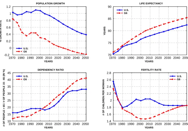
As portrayed in the top-left panel of Figure 3, the U.S. and the G6 have experienced a very different evolution of population growth rates. The growth rate has been substantially constant (around 1%) in the U.S. ever since 1970 whereas it has progressively decreased in
5
Gourinchas and Rey [2005] study the sustainability of the U.S. trade balance in light of the intertemporal approach to the current account and emphasize valuation effects associated to the rate of return. Bohn [2004]
finds evidence in favor of sustainability of the U.S.fiscal policy based on a test of the intertemporal government budget constraint. The level of the interest rate plays a crucial role for both results.
6
One exception is Caballero, Fahri and Gourinchas [2005], who also obtain a decreasing path for the real interest rate in their model.
1970 1980 1990 2000 2010 2020 2030 2040 2050 -0.2 0 0.2 0.4 0.6 0.8 1 1.2 YEARS % G R O W T H R A T E POPULATION GROWTH U.S. G6 1970 1980 1990 2000 2010 2020 2030 2040 2050 70 75 80 85 90 YEARS Y E A R S LIFE EXPECTANCY U.S. G6 1970 1980 1990 2000 2010 2020 2030 2040 2050 10 15 20 25 30 35 40 45 # O F P E O P L E > 6 5 / # O F P E O P L E 1 5 6 5 ( IN % ) YEARS DEPENDENCY RATIO U.S. G6 1970 1980 1990 2000 2010 2020 2030 2040 2050 1.4 1.6 1.8 2 2.2 2.4 2.6 2.8 # O F C H IL D R E N P E R W O M A N YEARS FERTILITY RATE U.S. G6
Figure 3: four demographic indicators.
the G6. Available projections point in the direction of a reduction in the U.S. growth rate starting in 2005. The declining trend is also expected to continue in the G6.
Population growth rates represent only one possible indicator of demographic trends. The top-right panel of Figure 3 reports the years of life expectancy for the U.S. and for the G6. The two bottom panels of Figure 3 respectively plot the dependency ratio and the fertility rates for the two economies. The dependency ratio is defined as the total number of individuals 65 years and older divided by the total number of individuals between 15 and 64 years of age. It represents a measure of dependency of the elderly on the fraction of the total population able to participate in the labor force.7 The fertility rates, the average number of children per woman in a given year, also confirm the overall declining demographic trends.
Two main points emerge clearly from this picture. First, lower population growth rates
7
The dynamics of the dependency ratio play a very important role for public policy decisions concerning welfare programs. See, for instance, Attanasio, Kitao and Violante [2005] for an assessment of social security reforms in the light of the projected demographic trends.
1980 1984 1988 1992 1996 2000 2004 -7 -6 -5 -4 -3 -2 -1 0 1 2 T O T A L B A L A N C E % O F G D P YEARS
TOTAL GOVERNMENT BALANCE
1980 1984 1988 1992 1996 2000 2004 20 25 30 35 40 45 50 55 60 65 70 D E B T % O F G D P YEARS NET GOVERNMENT DEBT U.S.
G6
U.S. G6
Figure 4: two measures of fiscal policy.
and faster population aging is a phenomenon that concerns the U.S. as well as the G6. Second, the differentials in demographic indicators, which were quite small at the beginning of the 1970s, have become more pronounced during the last two decades and are projected to remain as such at least until 2050, with the G6 ahead of the U.S. by several decades. Both considerations turn out to be important for the quantitative analysis in this paper.
The second piece of evidence that I present in this section covers the evolution of the total government balance and the stock of net government debt from 1980 until 2004. As mentioned in the introduction, demographic trends are crucial in this paper to reconcile the idea that fiscal deficits entail external imbalances (the twin-deficits hypothesis) with the puzzling fact that the U.S. fiscal consolidation that took place in the 1990s was accompanied only by an initial small correction in the trade deficit followed by a fast deterioration thereafter. The key question in the debate about Ricardian equivalence and the real effects of fiscal policy is whether financing a certain level of spending with taxes or debt matters for aggregate consumption. For this reason, I concentrate on fiscal deficits and government debt rather than on government spending.8
Figure 4 reports the total government balance (left) and the net government debt (right)
8A constant ratio of government spending to GDP is also roughly consistent with the evidence for G7
for the U.S. and for the G6 as a fraction of their GDP levels. Both panels suggest a split of the sample in three parts. Thefirst period corresponds to the 1980s and early 1990s. In those years, the U.S. was running a relatively expansionary fiscal policy. Fiscal deficits were on average about two percentage points higher than in the G6 and net government debt doubled to reach 60% in 1993. The second period roughly covers the 1990s. The main feature of that decade is thefiscal consolidation that took place in the U.S. and the increase in government debt in the G6. Beginning in 2000,fiscal policy in the U.S. has been again on an expansionary path relative to the G6. The rapid turnaround in the government balance hasfinally brought the U.S. deficit to the levels of the G6 at the end 2004.
The data highlight two regularities. First, fiscal stances follow similar patterns in the two regions, with two periods of expansion in the 1980s and during the lastfive years, spaced out by the consolidation of the 1990s. Second, the differentials for both deficits and debt levels appear to be small in magnitude. These two observations constitute the key aspects of fiscal policy for the following analysis.
3
A Life-Cycle Model of the U.S. and the G6
In this section, I set up a two-country world economy in which agents exhibit life-cycle behavior. An open economy represents the natural framework to think about the effects of demographics on the trade balance. A two-country model reveals particularly appropriate to the extent that the U.S. and the G6 are two major players in the world economy and is also instrumental to discuss the link between demographic factors and the real interest rate. Finally, the life-cycle structure not only naturally captures the key elements of the demographic transition but it also permits to consider non-Ricardian effects of fiscal policy.
The main difference with respect to the existing literature on computable life-cycle models concerns the tractability of the framework. I present a model in which the heterogeneity implicit in the life-cycle can be summarized by two state variables, the distribution of assets between retirees and workers and the ratio between the number of individuals in those two groups. This formulation adds life-cycle behavior on top of a basic structure close to the work of Blanchard [1985] and Weil [1989]. The framework is tractable enough to derive a closed form solution for aggregate consumption given prices, along the same lines of Gertler [1999]. This result is crucial to describe the basic mechanisms that underlie the effect of demographic factors on the trade balance.
identical in all respects. I describe in details the structure of the Home economy. Whenever necessary, I refer to Foreign variables with an asterisk “∗”. At time t, the Home country is populated by a continuum of agents of mass Nt. The commodity space is constituted by a
single consumption good which can be traded internationally at no shipping cost and serves as numeraire. There is no aggregate uncertainty. All agents have perfect foresight but can be surprised by unexpected exogenous shocks.
Individuals are born workers (denoted by the superscript w) and retire with probability
ω, which I assume to be fixed throughout the analysis. Once a retiree (denoted by the superscript r), an individual survives from period t to period t+ 1 with probability γt,t+1. The number of workers in period t is Ntw. In each period (1−ω+nt,t+1)Ntw individuals
(workers) are born. The law of motion for the aggregate labor force is
Ntw+1= (1−ω+nt,t+1)Ntw+ωNtw = (1 +nt,t+1)Ntw, (1)
so that nt,t+1 represents the growth rate of the labor force between period tand t+ 1. The
number of retirees is denoted by Ntr and evolves over time according to
Ntr+1= (1−ω)Ntw+γt,t+1Ntr. (2)
The ratio between the number of retirees and the number of workers, defined asψt≡Ntr/Ntw, summarizes the heterogeneity in the population. The variableψtis called “dependency ratio” and follows a law of motion that can be derived from expression [2] after dividing both sides by Ntw and rearranging using [1]
(1 +nt,t+1)ψt+1= (1−ω) +γt,t+1ψt. (3)
The growth rate of the number of retirees can also be derived from expression [2]
Ntr+1 Ntr = 1−ω ψt +γt,t+1= (1 +nt,t+1) ψt+1 ψt , (4)
where the second equality makes use of [3]. Finally, total population grows according to
Nt+1 Nt = (1 +nt,t+1) ¡ 1 +ψt+1¢ (1 +ψt) . (5)
also constant and equal to
ψ= 1−ω
1 +n−γ. (6)
The number of retirees relative to the number of worker depends positively on the probability of surviving and negatively on the probability of retirement and on the growth rate of the labor force. Under stationary demographics, from [4] and [5], it follows that the number of retireesNtr and the total populationNtgrow at the same rate as the number of workers Ntw,
which is equal to n.
Workers supply inelastically one unit of labor and retirees do not work.9 Individual pref-erences belong to the recursive non-expected utility family, originally introduced by Kreps and Porteus [1978] and extended by Epstein and Zin [1989] to an infinite horizon framework. The general formulation for an individual of cohort z={w, r} reads as
Vtz =n(Ctz)ρ+βzt,t+1£Et ¡ Vtα+1 |z¢¤ ρ α o1 ρ , (7)
whereCtzdenotes consumption andVtz stands for the value of utility in periodt. The discount factor of a retiree differs from that of a worker in order to account for the probability of death
βzt,t+1= ⎧ ⎪ ⎨ ⎪ ⎩ βγt,t+1 ifz=r β ifz=w
The preferences in [7] feature the well-known property of separating intertemporal substitu-tion from risk-aversion. The parameterρmeasures intertemporal substitution. In particular, the elasticity of intertemporal substitution is given byσ≡1/(1−ρ). On the other hand, the parameterαcaptures risk aversion. More specifically, the coefficient of relative risk aversion is equal to 1−α.
The expectation of Vt+1 differs across cohorts because the future value of utility depends
on the current employment status. In particular, a worker remains in the labor force with probabilityω and retires with probability 1−ω. The resulting expression for the expectation
9
It is possible to relax both these assumptions without sacrificing the analytical tractability of the model. See Gertler [1999] for details.
of next period’s value function is Et © Vtα+1|zª= ⎧ ⎪ ⎨ ⎪ ⎩ ¡ Vtr+1¢α ifz=r ω¡Vw t+1 ¢α + (1−ω)¡Vr t+1 ¢α ifz=w
The fact that the probability of retirement and death are independent of age makes it possible to consider the problem of a generic individual within each cohort without specific reference to her age or to her retirement period. In what follows, I discuss two additional assumptions that keep the model analytically tractable and greatly facilitate aggregation.
The idiosyncratic uncertainty about the lifetime horizon is eliminated by assuming the existence of a perfect annuity market in which retirees can fully insure against the risk of death. Retirees turn their wealth over to a perfectly competitive mutual fund industry which invests the proceeds and pays back a premium over the market return to compensate for the probability of death.10 For a retiree who survives between periodt−1 and t, the return on a one dollar investment is RW,t/γt−1,t, where RW,t is the world interest rate that clears the
international capital markets. The extra-return over the market rate compensates for the probability of death.
The idiosyncratic uncertainty about employment tenure is limited by imposing that house-holds are risk-neutral with respect to variations in income. To this extent, I set α = 1 in [7]. For a given level of the interest rate, only average consumption tomorrow (appropriately weighted) matters for current consumption decisions.
The assumption of perfect insurance markets against the risk of death is quite common in the literature (see, for instance, Yaari [1965] and Blanchard [1985]). A similar mechanism to insure against labor incomefluctuations would smooth consumption perfectly across work and retirement, hence shutting off the life-cycle channel which is at the very heart of the analysis. On the other hand, the assumption of risk neutrality, while still allowing for an arbitrary elasticity of substitution σ, mitigates the artificially high degree of labor income fluctuations induced by the constant transition probability into retirement.
I now turn to characterizing the consumption-savings problem for each cohort. I present the problem of a generic workerfirst and then the problem of a generic retiree.
10It is convenient to assume that in each country the mutual fund operates at the national level only.
The reason is that, in the presence of cross-country differences in aging profile, no arbitrage would imply equalization of returns in the insurance market but not in the capital market. Since the mutual fund industry is a device to keep the model tractable, the restriction in international insurance markets appears to be appropriate.
Workers. Individuals are born workers and start their life with zero assets. A generic worker ichooses consumptionCtw(i) and assetsAwt+1(i) to solve
Vtw(i) = max ©(Ctw(i))ρ+β£ωVtw+1(i) + (1−ω)Vtr+1(i)¤ρª
1
ρ, (8)
subject to
Awt+1(i) =RW,tAwt (i) +Wt−Ttw−Ctw(i), (9)
where Wt represents the market wage and Ttw is the total amount of lump-sum taxes paid
by a single worker. The function Vtr+1(i) (defined below) enters the continuation value of a worker to discount the possibility that retirement occurs between time tand t+ 1.
Retirees. A retiree j chooses consumption Ctr(j) and assetsArt(j) to solve
Vtr(j) = max ©(Ctr(j))ρ+βγt,t+1£Vtr+1(j)¤ρª 1 ρ, (10) subject to Art+1(j) = RW,tA r t(j) γt−1,t −C r t (j). (11)
There is no public pension scheme and the only source of income for retirees is financial wealth.11
Firms. Firms operate in perfect competition using a constant returns to scale technology
with no adjustment costs. The aggregate production function is Cobb-Douglas
Yt= (XtNtw) α
Kt1−α, (12)
whereα∈(0,1) is the labor share andXtstands for exogenous labor-augmenting productivity
which grows at the constant ratex. In order to be consistent with the notation adopted so far, I assume that households own the capital stock but thatfirms bear the cost of depreciation
δ.
Government. The government levies lump-sum taxes and issues one-period debt Bt+1 to
finance a given amount of spending Gt according to the flow budget constraint
Bt+1=RW,tBt+Gt−Tt, (13)
11
Gertler [1999] studies the effects of moving from a public to private pension system in a closed economy with the life-cycle structure adopted in this model.
where Tt=NtwTtw represents the total tax revenues.
The Foreign country has a completely symmetric structure.
4
Equilibrium in the World Economy
The environment is competitive and all agents take prices as given. Formally, a competitive equilibrium is a sequence of quantities and prices such that in each country (i) households maximize utility subject to their budget constraint, (ii)firms maximize profits subject to their technology constraint, (iii) the government chooses a path for taxes and debt, compatible with intertemporal solvency, tofinance an exogenous level of total spending, (iv) goods and asset markets clear at the world level.
I can now describe in details the equations that constitute the competitive equilibrium. Again, the focus is on the Home country. For simplicity, I start from the problem of a retiree. As demonstrated by Farmer [1990], under the assumption of risk neutrality in preferences [7], the solution of the individual problem consists of an explicit decision rule for consumption, given prices and policy variables.12A retiree consumes optimally a fraction out of total wealth according to
Ctr(j) = ξtRW,tA
r t(j)
γt−1,t . (14)
From the Euler equation, it is possible to show that the marginal propensity to consume evolves according to
ξt= 1−γt,t+1βσRσW,t−1+1 ξt
ξt+1, (15)
The crucial point of equation [15] is that the marginal propensity to consume for a retiree is independent of individual characteristics. Indeed, the evolution ofξt is governed only by the world interest rate (an aggregate variable) and the probability to survive (identical across retirees).
The solution for the problem of a worker can be characterized along similar lines. Workers consume out offinancial and human wealth according to
Ctw(i) =πt[RW,tAwt (i) +Htw(i)], (16)
whereπt is the marginal propensity to consume for a worker. As for retirees, from the Euler
12The details of the derivation are provided in the appendix. See also Backus, Routledge and Zin [2004] for
equation, it is possible to retrieve the law of motion of the workers’ marginal propensity to consume πt= 1−βσ(Ωt+1RW,t+1)σ−1 πt πt+1 , (17) whereΩt≡ω+ (1−ω) 1 1−σ
t and t≡ξt/πtare two additional variables that link the marginal
propensities to consume of the two cohorts.13 Also for workers, the marginal propensity to consume only depends on aggregate or cohort-specific variables but not on individual characteristics. The variableHtw(i) in [16] represents the present discounted value of current and future human wealth net of taxation, that is
Htw(i)≡ ∞ X v=0 Wt+v−Ttw+v v Q s=1 (Ωt+sRW,t+s/ω) =Wt−Ttw+ Htw+1(i) Ωt+1RW,t+1/ω . (18)
The term Ωt+1RW,t+1/ω constitutes the effective discount rate for a worker. The first
com-ponent of the higher discounting captures the effect of the finite lifetime horizon (less value attached to the future). The actual discount factor is also increased by the term ω which induces higher savings to finance consumption during the retirement period (positive proba-bility of retiring). I now proceed to derive the aggregate consumption function.
The first step consists of aggregating consumption by cohort, which is possible because in-dividuals within the same cohort share the same marginal propensity to consume. Aggregate variables take the formZtr≡RNtr
0 Ztr(j)dj for retirees and Ztw ≡ RNw
t
0 Ztw(i)di for workers.
Aggregate consumption for retirees is given by
Ctr=ξtRW,tArt, (19)
where Ar
t is total wealth that retirees carry from period t−1 into period t, with aggregate
return given by RW,t.14
Individual consumption for workers can be aggregated along the same lines to yield
Ctw =πt(RW,tAwt +Ht), (20)
13
In the appendix, I formally show that and Ω are both larger than one in steady state. For plausible parameter choices, including the calibration adopted in the numerical experiment section, this result holds also outside the steady state. The fact that t>1 implies that the marginal propensity to consume is higher
for retirees than for workers. As the next section clarifies, this result constitutes a key element to understand the response of consumption and savings to changes in demographic factors.
14
Each individual retiree earns a return given byRW,t/γt−1,t but only a fractionγt−1,tof retirees survive
whereAw
t is total aggregatefinancial wealth held by workers. The aggregate value of human
wealth evolves according to
Ht=NtwWt−Tt+
Ht+1
(1 +nt,t+1)Ωt+1RW,t+1/ω
. (21)
The second step consists of writing the aggregate consumption function Ct as the sum of
[19] and [20]. I denote by λt≡Art/At the share of total assetsAtheld by retirees. It follows
that the aggregate consumption function
Ct=πt[(1−λt)RW,tAt+Ht+ tλtRW,tAt]. (22)
Finally, I need to characterize the evolution of the distribution of assets, as captured by
λt. This additional state variable keeps track of the heterogeneity in wealth accumulation
introduced by the life-cycle hypothesis. Aggregate assets for retirees depend on the total savings of those who are retired in period t but also on the total savings of the fraction of workers who retire betweent and t+ 1
Art+1 =RW,tAtr−Ctr+ (1−ω) (RW,tAwt +NtwWt−Tt−Ctw). (23)
Aggregate assets for workers depend only the savings of the fraction of workers who remain in the labor force
Atw+1 =ω(RW,tAwt +NtwWt−Tt−Ctw). (24)
After substituting expressions [19] and [24] into [23], I exploit the definition of λt to obtain
the law of motion for the distribution of wealth across cohorts
λt+1At+1 = (1−ω)At+1+ω(1−ξt)RW,tλtAt. (25)
Expression [25] relates the evolution of the distribution of wealth λt to the aggregate asset
position At.
The problem of thefirm is standard. Firms hire labor to the point that the real wage equals the marginal product of labor
Wt=α
Yt
Ntw. (26)
The investment decisions are consistent with the condition that the marginal product of capital, net of depreciation, equals the real return that prevails in the international asset
markets
RW,t= (1−α)
Yt
Kt
+ (1−δ). (27)
Finally, in equilibrium, the government is bound to choose combinations of taxes and debt that respect the intertemporal solvency condition
RW,tBt= ∞ X v=0 (Tt+v−Gt+v) v Q s=1 RW,t+s . (28)
The current value of debt (principal and interests) must be equal to the present discounted value of current and future primary surpluses. For later purposes, it is also convenient to expressfiscal policy variables as fractions of GDP. Given the path for Gt, I assume that the
government fixes the ratiogt≡Gt/Yt and chooses combinations of tax ratesτt≡Tt/Yt and
debt-to-GDP ratios bt≡Bt/Ytthat satisfy [28].
So far, I have described the behavior of the private sector and of the government of the Home country. The Foreign country is characterized by a similar set of relations. I now complete the characterization of the equilibrium by discussing how the asset and goods markets clear. The portfolio of assets held by the private sector is composed by capital, government bonds and net foreign assets
At=Kt+Bt+Ft. (29)
The difference between production Yt and domestic absorption (Ct+It+Gt) defines net
export as
N Xt=Yt−(Ct+It+Gt), (30)
where investment is given by
Kt+1=It+ (1−δ)Kt. (31)
The evolution of net foreign assets links the goods and the asset markets together. Net foreign assets represent the payment received from the rest of the world in exchange for exporting
goods.15 Hence,F
t evolves according to
Ft+1 =RW,tFt+N Xt. (32)
International capital flows equalize the return RW,t across countries. The model is closed by
the equation that characterizes the equilibrium in the market for international debt
Ft+Ft∗ = 0.
Despite the tractability of the model, a complete closed form solution cannot be derived. In the appendix, I characterize a symmetric steady state of the model in which exogenous variables are constant and equal across countries. Given the presence of exogenous growth, quantities are not stationary. A steady state with balanced growth exists for detrended variables, that is, for variable expressed in terms of efficiency units XtNtw. In such a steady
state, quantities grow at the constant rate (1 +x) (1 +n) ∼= 1 +x+n. In what follows, I denote a generic variableZtin terms of efficiency units by lower case letterszt≡Zt/(XtNtw).
The solution for the steady state and for the transition dynamics is obtained by employing a non-linear Newton method.16 In order to have a determinate steady state, I calibrate from
the data an initial level of steady state government debt relative to GDP as the “fiscal rule” which closes the model.
As a final remark, it is interesting to note that in this model the steady state is determi-nate.17 The life-cycle structure pins down endogenously the steady state value of net foreign asset. Ghironi [2003] shows a similar result in a framework with overlapping families of infinitely lived agents based on Weil [1989].
15
Following Obstfeld and Rogoff[1996], the current account balance can be defined as the one-period vari-ation in the net foreign asset position
CAt≡Ft+1−Ft= (RW,t−1)Ft+N Xt.
For the U.S., the current account and trade balance essentially coincide, which means that the net interest rate payment on the outstanding stock of net foreign assets must be small. Lane and Milesi-Ferretti [2001] and Gourinchas and Rey [2005], among others, discuss extensively these valuation effects.
16See Juillard [1996] for details about the implementation of the specific Newton-Raphson algorithm used
to solve the model.
17It is well known that open economy models with incomplete markets generally feature steady state
in-determinacy and non-stationary dynamics of net foreign assets. See Schmitt-Groh´e and Uribe [2003] for the discussion of a number of alternative mechanisms to circumvent this problem.
5
The Determinants of the Trade Balance
The analytical tractability of the life-cycle framework presented in the previous two sections allows to isolate the determinants of the trade balance and to sort out precisely the equilibrium effect of demographic factors and fiscal policy on each component.
The assumption of perfect financial market integration implies that in each period capital in efficiency units must be equal across countries. The result follows from the no arbitrage relation
RW,t−1 +δ = (1−α) (kt)−α= (1−α) (kt∗)−α, (33)
which entailskt=k∗t,∀t. Since both countries have access to the same technology, also output
per efficiency unit is equalized across borders (yt=yt∗). Assuming thatgt=g∗t, the national
account identity [30] gives an expression for the trade balance as a function of consumption and investment differentials18
nxt=−
1
2(cR,t+iR,t), (34)
where for any zt and zt∗, I define zR,t≡zt−zt∗.
From [22] and its Foreign counterpart, relative consumption is
cR,t=RW,t{[πt(1−λt)at−π∗t(1−λ∗t)a∗t] + (ξtλtat−ξ∗tλ∗ta∗t)}+ (πtht−π∗th∗t) (35)
The first two components of [35] represent the differentials in the propensity to consume out of financial wealth by workers and retirees respectively. The third term captures the differentials in the propensity to consume out of human wealth.
From [31] and its Foreign country counterpart, the equality of the capital stock in efficiency units implies that relative investments correspond to
iR,t= ¡
nt,t+1−n∗t,t+1
¢
kt. (36)
I begin by highlighting the effects of population aging on the trade balance. For the sake of simplicity, it is useful to think of this experiment in isolation, holding constant population growth rates and government debt at their initial steady state values. In the absence of population growth rate differentials, iR,t = 0. From [34], savings differentials completely
18In what follows, I refer toc
R,t also as (the negative of) relative savings. The result is a consequence of
characterize the dynamics of the trade balance
nxt=−
1 2cR,t.
The adjustment of the trade balance to a change in the degree of population aging de-pends primarily on the response of the marginal propensities to consume. Different marginal propensities to consume within the same cohort across countries reflect different degrees of population aging between the Home and the Foreign economy.
In the model, the effects of population aging can be studied in relation to variations in the probabilities of survival γ and γ∗. In steady state, the relative marginal propensity to
consume for retirees is
ξR=−βσRWσ−1(γ−γ∗).
Faster aging in one country is associated with a relatively more pronounced decrease in the marginal propensity to consume. While population aging also entails general equilibrium effects on the world interest rate, aging differentials only affect relative savings.
The effect of aging on the relative marginal propensity to consume for workers propagates through the terms Ωand Ω∗
πR=−βσRσW−1 h
(Ω)σ−1−(Ω∗)σ−1i.
In the appendix, I show formally that, for a given interest rate, a higher surviving probability induces a reduction in the marginal propensity to consume for workers too. As before, different surviving probabilities across countries only influence relative savings.
Intuitively, an increase in the expected lifetime horizon brings about two effects. First, an individual who is in the labor force at the moment of the shock increases her savings to finance a longer retirement period. Second, after retirement, agents spread their consumption over an extended period. While it is still true that the marginal propensity to consume is higher for a retiree than for a worker, the consumption level of both cohorts decreases as compared to before the shock. Most importantly, in relative terms, the level of savings is higher in the country with higher life expectancy. The relative excess of savings generates a trade surplus associated with the accumulation of a positive stock of net foreign assets. The life-cycle structure of the population is at the core of this mechanism. The difference in the marginal propensities to consume is a result of the heterogeneity between workers and retirees. Despite the assumptions made to limit the degree of heterogeneity within each cohort and maintain analytical tractability, the model still preserves the key ingredients of
standard life-cycle frameworks and provides a transparent illustration of the forces at work. Alongside the effects on the marginal propensity to consume, a higher probability of survival also increases the dependency ratio. From [6], in steady state, the cross-country differential is
ψR= (1−ω) (γ−γ
∗)
(1 +n−γ) (1 +n−γ∗).
Quite obviously, the dependency ratio is higher in the country with longer life expectancy. Since retirees have a higher marginal propensity to consume relative to workers, over time this effect partly offsets the initial fall of aggregate consumption. Nonetheless, for plausi-ble parameterizations, the reduction of the marginal propensity to consume among retirees dominates the cross-sectional adjustment within each country.
Finally, the excess of total savings generates a drop in the interest rate. The absolute drop depends on the overall change in the lifetime horizon. In particular, the longer the retirement period, the larger the effect on workers and retirees savings. The effect of population aging appears to be crucial to explain the declining trend in the real interest rate during the last twentyfive years.
I shall now discuss the impact of population growth rate differentials. As for the previous experiments, it is useful to fix the other sources of variations, in this case fiscal deficits and population aging, at their initial steady state values. In steady state, total population Nt
grows at the same rate as the labor force Ntw. During the transition, the link between the two growth rates in the Home country is governed by
Nt+1 Nt
= (1 +nt,t+1) + (1−ω) +γψt
1 +ψt .
The primitive shocks for this experiment are the labor force growth rates in the two countries (nand n∗).
The direct channel of transmission of population growth rate differentials operates through the investment sector. From equation [36], a smaller population growth rate in one region shifts relative investment towards the rest of the world. The no arbitrage relation [33] repre-sents the driving force behind this adjustment. In frictionless internationalfinancial markets, the rate of return must be equal across countries. Capital flows towards the region with a relatively larger pool of workers ensure no arbitrage opportunities by employing capital where it is relatively more productive.19 If, for example, the Home country labor force grows
19
The importance of this channel depends on the assumption about the degree of capital mobility across countries. For example, the presence of adjustment costs in investment would limit the transmission of population growth rates shocks.
at a relatively higher rate, Foreign capital relocates to the more productive Home firms, in exchange for a claim on ownership. This mechanism results in an accumulation of net foreign debt by Home households and a negative trade balance (nxt<0).
The presence of life-cycle behavior partly acts to counterbalance the investment channel. A smaller growth rate of the labor force at timetalso implies an increase in the dependency ratio, which in turn leads to a reduction of the total population growth rate att+ 1. Holding fixed the probability of survival, aggregate consumption increases because retirees become relatively more numerous. In the absence of population aging, the marginal propensities to consume for both cohorts are equal across countries. While the general equilibrium effect of a shock to population growth rates on the interest rate reduces the marginal propensities to consume for both cohorts, the marginal propensity to consume for retirees rises relative to workers.
The sign of the net adjustment (investment versus consumption-saving decisions) is am-biguous. The numerical experiments in the next section suggest a mild predominance of the investment channel but the overall effect appears to be rather small.
Lastly, I consider the effects of fiscal deficits on the trade balance. In what follows, I shut off any demographic differential across countries. For the sake of the argument, it is also convenient to set the population growth rate equal to zero.20 In such circumstances, the
trade balance is again completely determined by relative savings
nxt=−
1 2cR,t.
The absence of life expectancy differentials implies that the marginal propensity to consume for each cohort is identical across countries. Expression [35] can be rewritten as
cR,t=πt[hR,t+RW,taR,t+ ( t−1)RW,t(λtat−λ∗ta∗t)]. (37)
Thefirst component of [37] is relative human wealth, which depends negatively on the relative tax rate hR,t=− ∞ X v=0 τR,t+vyt+v v Q s=1 [Ωt+sRW,t+s/(1 +x)ω] . (38)
The second term of [37] is the gross return on the relative aggregate asset position. From
20
This assumption permits to illustrate more starkly the non-Ricardian effects associated tofiscal policy in this framework. Weil [1989] shows that a positive population growth rate (overlapping families of infinitely lived agents) is a sufficient condition for Ricardian equivalence to fail in an otherwise neoclassical world.
expression [28] and [29], I can rewrite RW,taR,t= 2RW,tft+ ∞ X v=0 τR,t+vyt+v v Q s=1 [RW,t+s/(1 +x)] . (39)
Equation [39] follows from the fact that capital in efficiency units is equal across countries and that the Home and Foreign net foreign asset positions add up to zero. Finally, the third element of [37] captures relative asset holdings by retirees (remember thatλt=Art/At). From
expression [25], this difference evolves according to
λtat−λ∗ta∗t = (1−ω)aR,t+ω µ 1−ξt 1 +x ¶ RW,t−1 ¡ λt−1at−1−λ∗t−1a∗t−1 ¢ . (40)
In general, relative asset holdings by retirees can be expressed as a function of the cross-country difference in aggregate assets.21
The solution for the trade balance in the absence of cross-country demographic differentials clarifies the channel through which fiscal deficits influence the trade balance. Starting from a symmetric steady state, consider, for example, the case of a relativefiscal deficit in the Home country. This experiment corresponds to an increase of the debt-to-GDP ratio bt holding
constant the level of spending, so that the tax rate τt is reduced during the expansion. In
this scenario, on impact, the trade balance depends only on future relative tax rates. Since the Home country is running afiscal deficit, the relative tax rate is negative, boosting relative human wealth and turning the trade balance into a deficit. As time goes by, the tax rate in the Home country increases in order to smooth the tax hike that takes place at the end of the fiscal expansion. Along the transition, the tax cut stimulates private consumption and reduces private savings. In general equilibrium, the drop of the savings rate increases the real interest rate. This effect partially limits the benefits of the fiscal expansion on consumption. Fiscal deficits entail non-Ricardian effects because of the life-cycle structure of the economy. In expressions [38] and [39], relative taxes are discounted at different rates. In other words, a fraction of government debt constitutes net wealth for the private sector. Because of transition into retirement, a worker who benefits from a tax cut today, with some probability, will not be subject to the future higher tax rate, which is necessary, ceteris paribus, to satisfy the
21Whether expression [40] admits a backward or forward solution depends on the autoregressive coefficient
being larger or smaller than one. Fiscal and demographic forces will typically exert opposite effects on this term. For high enough values of the equilibrium interest rate, possibly due to expansionaryfiscal policies, the autoregressive coefficient will be larger than one so that only current and futurefiscal decisions matter for the equilibrium trade balance.
government intertemporal solvency condition. Hence, the capitalization of future tax rates by workers is less than complete (as measured by the factor Ωt+v/ω). In this case,fiscal and
trade deficits are “twins”, although the synchronization is less than perfect. The persistence in the trade deficit is augmented by the term in [40], which measures the variation in the distribution of wealth across cohorts following an expansion and is peculiar of the life-cycle structure of the economy.
As a final remark, whenω = 1, the setup encompasses the standard infinite horizon model with a representative agent. Under this limiting case, agents never retire so thatλt=λ∗t = 0.
Since alsoΩt= 1∀t, Ricardian equivalence holds and the trade balance is only a function of
the (relative) level of public spending, not of the financing decisions (debt versus taxes).
6
A Quantitative Investigation of the U.S. Trade Deficit
In this section, I evaluate the quantitative significance of the different effects discussed above. The objective is to assess the overall contribution and the relative importance of demographic factors and fiscal deficits in accounting for the evolution of the U.S. trade balance vis-a-vis the G6 after the breakdown of Bretton Woods. The application of the theoretical apparatus developed so far leads to three main results:
1. The demographic differentials between the U.S. and the G6 explain the declining trend of the U.S. trade deficit in the last three decades.
2. The consideration of demographic factors reconciles the evolution offiscal policy in the U.S. and in the G6 with the dynamics of the trade balance.
3. The demographic transition generates a path of the world real interest rate broadly consistent with the data.
The time period is one year. The demographic transition starts in 1970 and convergence for population growth rates22 occurs in 2030. The choice of 1970 as the base year depends upon two facts. First, the assumption of perfect capital markets appears to be the most appropriate for the period after the collapse of Bretton Woods in the early 1970s. Second, in those same years, demographic differentials between the U.S. and the G6 were also minimal. It seems then reasonable to start from a symmetric steady state in which trade is balanced and
22In order to avoid that, in the limit, one country ends up representing the entire world economy, I consider
evaluate the impact of fiscal deficits and demographics without adjustment effects induced by an existing stock of assets or liabilities. In the section on robustness, I discuss alternative initial steady states as well as different convergence scenarios.
Initial Steady State. The calibration of the demographic variables is based on previous
studies and on data from the United Nations World Population Prospects: The 2004 Revision. Population grows at a rate of 1%, which is in line with the observed value for both regions in 1970. Individuals are assumed to enter the economy as workers at the age of 20 and work on average (1−ω)−1 years. I choose the parameter ω = 0.9778 to match a 45-year average permanence in the labor force, which corresponds to the working period used by Auerbach and Kotlikoff[1987]. I set the surviving probability for a retiree (γ) equal to 0.8, in order to match the average expected lifetime horizon of an agent in the model (65 + (1−γ)−1) to the empirical counterpart in 1970, which was roughly 70 years both for the U.S. and G6.
The choice of the values for preference and production parameters is mostly in line with the existing literature. The elasticity of intertemporal substitution σ is assumed to be equal to 0.5, which represents a compromise between the values usually adopted in the publicfinance literature (e.g. Auerbach and Kotlikoff[1987]) and in the real business cycle literature (e.g. Cooley [1995]).23 The discount factorβ is set residually equal to one24 in order to obtain a real interest rate of 5% in 1970. The production parameters take values in line with the real business cycle literature. The labor shareα is assumed to be 2/3, the depreciation rate δ is set to 6% and technology grows at 1%.
Throughout the analysis, I focus on the governmentfinancing decisions of a constant level of public expenditure. Ifix the ratio of government spending to GDP to 20%, which corresponds approximately to the average U.S. value during the post-war period,25 as reported by the Bureau of Economic Analysis. The ratio of government debt to GDP is calibrated using data on net debt from the International Monetary Fund (World Economic Outlook Database), which are available only starting in 1980. I set the ratio of debt to GDP in the initial symmetric steady state to 26%, which represents the average between U.S. and G6 in 1980. For the U.S., this value represents a reasonable approximation also for the 1970s, a decade
23
See Attanasio [1999] for a comprehensive survey.
24A value of the subjective discount factor equal to one is consistent with the estimates in Hurd [1989]. 25This value obviously underestimates the role of government spending in European countries and Japan.
However, the model excludes features, such as a public pension system or a public health system, which account for large parts of government spending in those countries and are likely to provide utility to households. Hence, the value of 20% seems a reasonable approximation in a context in which government spending is considered pure waste.
during which the ratio of net debt to GDP was roughly constant.26 In the baseline experiment,
I assume that the ratio of debt to GDP is constant at 26% also in the G6 throughout the 1970s. In the section on robustness, I consider an extended time series for the G6 extrapolated from gross government debt as reported by the OECD Economic Outlook Database.
Table 1. initial symmetric steady state
n 1% population growth rate
(1−ω)−1 45 avg. working period (years)
(1−γ)−1 5 avg. retirement period (years)
β 1 subjective discount factor
σ 0.5 elasticity of intertemporal substitution
α 2/3 labor share
δ 6% depreciation rate
x 1% growth rate of technology
g 20% government spending (% of gdp)
b 26% government debt (% of gdp)
Given the benchmark calibration, the model delivers a capital-income ratio equal to 3 in the initial steady state. Investment constitutes 24% of GDP and the tax rate is equal to 20.8%.
Final Steady State. The transition from the initial to thefinal steady state is governed by
the evolution of demographic factors (expected lifetime horizons and population growth rates) and of fiscal stances (debt-to-GDP ratios) in both countries. Convergence for population growth rates occurs in 2030 at a value equal to 0.2%, in the baseline experiment, which coincides with the average of the U.N. projections for the U.S. and the G6 for the period 2030−2050. The U.N. projections also constitute the anchor for the lifetime expectancy in both regions in the same period. The implied values of the average retirement period are 15 and 18 years for the U.S. and G6 respectively. For debt-to-GDP ratios, I use the projected values for 2006 from the IMF World Economic Outlook Database, approximately equal to 50% in the U.S. and 70% in the G6.
26Data on net debt for the U.S. are available also from the Congressional Budget Office for the entire post war
period. While the pattern is essentially the same, there exist some differences in terms of absolute magnitudes, although the order never exceeds 5%. For international comparisons, the World Economic Outlook Database appears to be the most reliable source for the time series of net debt.
Table 2. final steady state
u.s. g6
n 0.2% 0.2% population growth rate
(1−γ)−1 15 18 avg. retirement period (years)
b 50% 70% government debt (% of gdp)
The Experiment. The central numerical experiment of the paper consists of simulating
an unexpected shock to demographic variables andfiscal stances in 1970 and to compute the transition path to the final steady state, which is reached in 2030. Under perfect foresight, agents are surprised by the shock in the initial period but perfectly anticipate the evolution of the exogenous variables thereafter. I discuss the likely implications of this assumption below. I use the realized values of net debt as a percentage of GDP in the two countries as the exogenous fiscal stances in the simulation. Given the constant level of government spending as a fraction of output, the tax rate and the government surplus are an outcome of the model which depends on the equilibrium output and interest rate. I compute the probability of surviving from the data on life expectancy under the assumption that the average permanence in the labor force is constant at 45 years. Finally, I infer the growth rate of the labor force from the data on population growth rates, adjusting for convergence in 2030 at 0.2%.
Results. Figure 5 compares the series of the trade balance as percentage of GDP generated
by the model with the trend of the HP-filtered series of the U.S. trade balance vis-a-vis the G6 for the period 1980−2004.
The time series of the trade balance exhibits three key periods. The first segment, which includes the first “dip” in the trend, begins in the early 1980s and lasts for slightly less than a decade. The second part of the series covers the years from the late 1980s to the mid 1990s and is characterized by a small reduction in the trade deficit. Finally, the third period, which approximately starts in the second part of the 1990s and continues as of today, displays a further worsening of the trade deficit towards 2% of GDP.
The model performs reasonably well to explain the long run movements of the U.S. trade balance vis-a-vis the G6. It captures the overall declining trend, the prolonged period of sustained deficits and the key swings in the last twentyfive years. The fraction of the trend explained by the model reduces over time but this aspect is most likely associated with the assumption of perfect foresight which leads to a more pronounced adjustment at the beginning of the experiment.
1980 1984 1988 1992 1996 2000 2004 -2 -1.8 -1.6 -1.4 -1.2 -1 -0.8 -0.6 -0.4 -0.2 0 YEARS T R A D E B A L A N C E % O F G D P
THE U.S. TRADE BALANCE: MODEL SIMULATION vs. LOW FREQUENCY COMPONENT
MODEL DATA (TREND)
Figure 5: the u.s. trade balance - simulation and data (trend).
The central argument of the paper revolves around the decomposition of the simulated trade balance series, reported in Figure 6. I repeatedly shut offall but one source of variation and compute the trade balance implied by the model under the a single shock. In what follows, I discuss the two main results of this exercise and I complete the analysis with the general equilibrium implications of the demographic transition.
Result #1. Demographic differentials explain the negative trend of the U.S. trade balance.
The demographic transition generates the negative trend of the trade balance observed in the data. As illustrated by Figure 6, the differentials in life expectancy account for most of the adjustment.
The intuition behind these effects hinges upon the discussion of the previous section. The response to the observed demographic transition requires the Home country to run a persistent trade deficit that accommodates the excess of savingsflowing in from the rest of the world. While aging and smaller growth are a global phenomenon, the cross-country differentials are the key determinant of the equilibrium trade balance. In the Foreign country, workers save relatively more to cope with a longer retirement period and retirees spread their consumption over a relatively longer horizon.
The simulation also shows that the strength of the investment channel by itself is quan-titatively limited. On the one hand, capital flows towards the Home country where it is
1980 1984 1988 1992 1996 2000 2004 -2 -1.5 -1 -0.5 0 0.5 1 YEARS T R A D E B A L A N C E % O F G D P DEMOGRAPHICS 1980 1984 1988 1992 1996 2000 2004 -2 -1.5 -1 -0.5 0 0.5 1 YEARS T R A D E B A L A N C E % O F G D P FISCAL POLICY 1980 1984 1988 1992 1996 2000 2004 -2 -1.5 -1 -0.5 0 0.5 1 YEARS T R A D E B A L A N C E % O F G D P LIFE EXPECTANCY 1980 1984 1988 1992 1996 2000 2004 -2 -1.5 -1 -0.5 0 0.5 1 YEARS T R A D E B A L A N C E % O F G D P POPULATION GROWTH DEMOGRAPHICS LIFE EXPECTANCY DEMOGRAPHICS POPULATION GROWTH FULL MODEL FISCAL POLICY FULL MODEL DEMOGRAPHICS
Figure 6: the determinants of the trade balance.
relatively more productive. On the other hand, however, holding constant life expectancy, smaller population growth rates reduce savings in the Foreign country.
In the case of variable surviving probability, a smaller population growth rate interacts with population aging to the extent that both effects push the dependency ratio in the same direction. The number of retirees grows relatively to the number of workers because (i) the average lifetime horizon is longer (aging) and (ii) less people are born in each period (growth). The combination of these two forces leads to a drop in the marginal propensities to consume which is stronger for the economy experiencing a more dramatic demographic transition.
Overall, the negative trend in the Home country trade balance is the result of demographic differentials that persist over time.
Result #2. Fiscal policy amplifies the trend induced by demographic differentials.
The second notable feature of the quantitative experiment is that fiscal deficits operate as an amplification mechanism on top of the trend generated by demographic factors.
Fiscal policy differentials cause the three major swings in the simulated trade balance which replicate quite closely thefluctuations in the observed trend during the last twentyfive years. It is important to stress that fiscal policy differentials, rather than absolute magnitudes, are the ultimate determinant of the equilibrium trade balance. In a two-country world, fiscal deficits in the Home country do not necessarily entail a Home country trade deficit. Absent demographic differentials, a fiscal deficit could be accompanied by a trade surplus simply because fiscal policy in the Foreign country is relatively more expansionary. This consideration bears the consequence that fiscal policy alone can hardly be the main driving force behind the realized U.S. trade deficit vis-a-vis the G6. Differential fiscal stances in the data are simply too small to support large trade deficits, as already pointed out in section 2. The bottom line of the analysis is that it is possible to reconcile the persistent U.S. trade deficits with the conduct of fiscal policy in the last twenty five years once demographic dynamics are properly taken into account. In this scenario, the overall picture of the U.S. trade balance vis-a-vis the G6 becomes fairly reasonable.
Result #3. The behavior of the real interest rate is broadly consistent with the data.
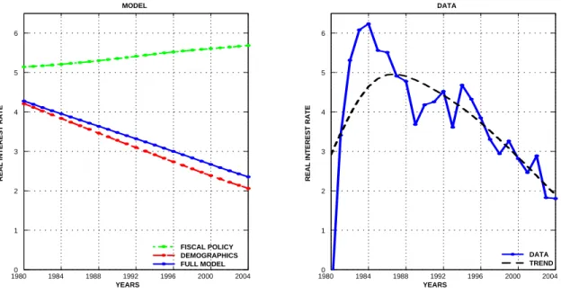
The demographic transition and the fiscal policy decisions in both regions carry important implications for the equilibrium world interest rate.
Figure 7 compares the world interest rate generated by the model as an outcome of the simulation discussed above with the data on the ex-post real interest rate for the G7 (from the IMF International Financial Statistics Database).
Contrary to the trade balance, the real interest rate is determined by global variables. The first lesson from Figure 7 is that demographic factors also play a critical role in accounting for the declining trend in the real interest rate. The excess savings associated with the increase in life expectancy at the world level drives the real interest rate downward. Second, fiscal deficits lead to an increase of the interest rate but the quantitative contribution is indeed modest.
These results shed new light on the empirical (lack of) relationship between fiscal deficits and interest rates. Evans [1987] suggests that the absence of high interest rates in periods of substantial fiscal deficits, both for the U.S. and at the international level, supports the hypothesis of Ricardian equivalence.27 The analysis in this paper implies that, even if fiscal deficits do trigger a positive response of the real interest rate, the failure to control for demographic trends might substantially bias the results.
19800 1984 1988 1992 1996 2000 2004 1 2 3 4 5 6 YEARS R E A L I N T E R E S T R A T E MODEL FISCAL POLICY DEMOGRAPHICS FULL MODEL 19800 1984 1988 1992 1996 2000 2004 1 2 3 4 5 6 R E A L I N T E R E S T R A T E YEARS DATA DATA TREND
Figure 7: the real interest rate - simulation and data.
Decreasing real interest rates generally favor deficits by reducing the cost of borrowing and maintaining a low burden of outstanding debt. This mechanism constitutes an intertemporal valuation effect for both net foreign debt and government debt which increases the persistence of existing deficits.
Figure 8 illustrates the valuation mechanism associated with low interest rates with two simple examples.
The left panel reports the response of the trade balance to an increase in life expectancy in the case of a two-country world and in the case of a small open economy which faces a constant interest rate. In the two-country model, the demographic shock hits the Foreign economy (γ∗ increases from 0.8 to 0.85 over 10 years) and generates a trade deficit in the Home country according to the mechanism discussed in the previous sections. For a small open economy, the same demographic transition generates a trade deficit in the rest of the world which, in this case, represents the Home country. The simulation shows that the general equilibrium effects associated with the interest rate absorb on impact half of the adjustment in the trade balance. Moreover, a decreasing interest rate implies that the trade balance is more persistent and that the rebalancing towards the new steady state occurs more gradually