Using Tensor Products to Detect Unconditional Label
Dependence in Multilabel Classifications
Jorge D´ıez∗, Juan Jos´e del Coz, Oscar Luaces, Antonio Bahamonde
Artificial Intelligence Center. University of Oviedo at Gij´on, 33204 Asturias, Spain http://www.aic.uniovi.es
Abstract
Multilabel (ML) classification tasks consist of assigning a set of labels to each
input. It is well known that detecting label dependencies is crucial in order
to improve the performance in ML problems. In this paper, we study a new
kernel approach to take into account unconditional label dependence between
labels. The aim is to improve the performance measured by a micro-averaged
loss function. The core idea is to transform a ML task into a binary classifica-tion problem whose inputs are drawn from a tensor space of the original input
space and a representation of the labels. In this joint feature space we define a
kernel to explicitly involve both labels and object descriptions. In addition to
the theoretical contributions, the experimental results of this study provide an
interesting conclusion: the performance in terms of Hamming Loss can be
im-proved when unconditional label dependence is considered, as our method does.
We report a thoroughly experimentation carried out with real world domains
and several synthetic datasets devised to analyze the effect of exploiting label
dependence in scenarios with different degrees of dependency.
Keywords: Multilabel, Label Dependence, Tensor products, Kernel methods
∗Corresponding author
Email addresses: [email protected](Jorge D´ıez),[email protected](Juan Jos´e
del Coz),[email protected](Oscar Luaces),[email protected](Antonio
1. Introduction
Inmultilabel(ML) classification tasks the aim is to assign, to each instance,
more than one class or label instead of a single one; the so-calledrelevantlabels.
This is the case of text categorization where items have to be tagged for
fu-ture retrieval. News or other kind of documents are annotated with more than
one label according to different points of view. Other application fields include
semantic annotation of images and video, functional genomics, music
catego-rization into emotions and directed marketing. Tsoumakas et al. in [27, 28] have made a detailed presentation of ML classification and their applications.
Probably one of the most popular approaches to tackle a ML classification
task is Binary Relevance (BR). It is the simplest one, but very effective for
some loss measures. Each label is classified as relevant or irrelevant by a binary
classifier independently learned for each label. Notice that BR does not consider
any relation between labels, making the learning assumption that labels are
independent. On the other hand, proper ML strategies try to take advantage
of correlation or interdependency between labels. The presence or absence of
a label in the set assigned to an instance depends on the feature values of the
instance, but it also depends on the relevance of the remaining labels. For example, it is very likely that labels “NBA” and “Los Angeles Lakers” appear
frequently together as tags for some videos of a sports website because there is
a strong relationship between both labels.
In this sense, two types of label dependence can be taken into account,
namely conditional and unconditional label dependence. See [5] for a complete
discussion of label dependence in ML classification. The difference between both
types of dependency is that conditional dependence captures the dependence
among labels given a particular example, whereas unconditional dependence is
a kind of global dependence, independent of any concrete observation. In the
previous example, it seems that the dependence between labels “Los Angeles Lakers” and “NBA” is mostly unconditional, no matter the actual content of
because the former is a franchise of the latter.
This paper presents a method based on capturing label dependence. The
main goal is that the algorithm takes into account, not only the descriptions of the objects, but also the dependency between each pair of labels. Lately, many
proposed ML classifiers exploit label dependence, see for instance [17, 22, 23].
Our approach is different from these methods cited previously because combines
together two factors: 1) it exploits unconditional label dependence instead of
conditional dependence which has been more studied in recent years, and 2)
it tackles ML classification as a structured output prediction problem [8, 26].
Our algorithm is a kernel method and the key element is a kernel to capture
unconditional label dependence. It is well known that kernel functions [24]
allow to efficiently represent input instances in a feature space, different from
the original input space. The proposed method incorporates a kernel over the space of labels, which it is combined with the kernel applied over the input
instances.
The performance of ML classifiers can be measured using very different loss
functions. When ML predictions are bipartitions of the set of labels (relevant
and irrelevant labels), loss functions are computed comparing subsets and
av-eraging scores. Taxonomically, loss measures can be divided into two groups:
example-based and label-based. The latter group includes also two versions
de-pending on how averages are computed: macro-averaged and micro-averaged
loss functions. Theoretically macro-averaged measures can be optimized
fol-lowing a decomposition approach, like BR. Another important characteristic of our method is that it is designed to optimize a complete family of loss
mea-sures for ML classification, namely micro-averaged loss functions. Our approach
can be applied to optimize any micro-average loss function whenever exists an
algorithm able to optimize such measure for binary classification.
Thus, the main contribution of this work is to propose a kernel-based ML
learner that is devised to induce classifiers aimed at improving the performance
in terms of a micro-averaged measure. Our proposal is based on two ideas:
whose inputs are drawn from a tensor space of the original input space and
a representation of the label space, and ii) to define a kernel that explicitly
incorporates both labels and object descriptions, in an attempt to exploit un-conditional label dependence. Despite this approach could be applicable for
any micro-averaged measure, we experimentally study its behavior in terms on
Hamming Loss, whose macro-averaged and micro-averaged versions coincide.
Interestingly, the experiments show that our proposal takes advantage of
con-sidering unconditional label dependence and obtains better Hamming scores
compared to making the assumption of label independence. This result is
inter-esting because it answers some questions raised in recent studies [5, 6] about if
exploiting label dependence could help to improve Hamming loss performance.
It also corroborates the results reported in [11], in which the authors investigate
whether Hamming scores can be improved if the distribution of test categories is known a priori. Here we use a different approach, we introduce additional
prior information in the form of a kernel for labels, but the conclusion is the
same: Hamming scores can be improved in some cases. Additionally, we show
that our kernel can be plugged into the algorithm proposed in [11] boosting its
performance in terms of Hamming loss.
After a formal presentation of ML learning tasks and hypotheses, we discuss
in detail label-based loss functions. Then, we derive a kernel method to optimize
micro-averaged measures. The paper ends reporting some experiments devised
to show the performance of such approach.
2. Multilabel Classification
Let L be a finite and non-empty set of labels {l1, . . . , lm}, let X be an
input space, and letY be the output space, the set of subsets of labels. A ML classification task can be represented by a dataset
D={(x1,y1), . . . ,(xn,yn)} ⊂ X × Y (1)
of pairs of inputs xi ∈ X and subsets of labels yi drawn from an unknown distribution. We identify the output spaceY with vectors of dimensionmwith
Table 1: Description of the most important symbols used in the paper
D Original ML training set D˜ Transformed training set fromD
x Input instance yi Labels associated with x
X Matrix of input spacesxofD Y Matrix of labelsy ofD
n Number of instances inD m Number of labels in D
X Input space Y Output space
p Dimension ofX L Set of labels
h Hypothesis (a ML classifier) l A label fromL
.. is transformed into ... el Vectorial representation ofl
⊗ Kronecker product δi,l Kronecker delta
I Identity matrix W Parameter vector of ˜h
lk Vector column of labelkinY ρ Correlation coefficient
µ(v) Mean of vectorv σ(v) Standard deviation of vectorv
components in{0,1}. In this sense, fory∈ Y,
l∈y and y[l] = 1
will appear interchangeably and will be considered equivalent. In the following,
we assume that the input space is a subset of the Euclidean space of dimension
p,
X ⊂Rp.
Then, we will refer to a learning task as a couple of matrices
D≡ X,Y
(2)
ofnrows andpandmcolumns respectively.
The goal of a ML classification task D is to induce a hypothesis defined as follows.
Definition 1. A ML hypothesis is a function h from the input space to the
output space, set of subsets (power set) of labelsP(L); in symbols,
h:X −→ Y=P(L) ={0,1}m. (3)
In other words,h(x)[l] = 1 means that labellis included in the set of predictions of the hypothesishfor inputx.
2.1. Loss Functions for Multilabel Classification
ML classifiers can be evaluated from different points of view. The predictions
can be considered as either as a bipartition or as a ranking of the set of labels. In
this paper the performance of ML classifiers will be evaluated as a bipartition.
Thus, loss functions must compare subsets of labels.
Usually these measures can be divided into two groups [28]. The
example-basedmeasures compute the average differences of the actual and the predicted
sets of labels over all examples. On the other hand, the label-based measures
decompose the evaluation into separate evaluations for each label. There are two
options here, averaging the measure label-wise (usually calledmacro-average),
or concatenating all label predictions and computing a single value over all of them, the so-calledmicro-averaged version of a measure.
For further reference, let us recall the formal definitions of these measures.
For a prediction of a multilabel hypothesish(x) and a subset oftruly relevant
labelsy⊂L, for each label l∈L we can compute the following contingency matrix:
y[l] = 1 y[l] = 0
h(x)[l] = 1 a(x, l) b(x, l)
h(x)[l] = 0 c(x, l) d(x, l)
(4)
Each of the functions in this matrix represents one of the four possible states
for a predicted label: a true positive (a), a false positive (b), a false negative (c) and a true negative (d). They have a value of 1 when the predicates of the
corresponding row and column are both true, otherwise the value is 0. Notice for
the truly relevant labell. Furthermore, for a particular pair (x, l) only one of the entries of the matrix is 1, the rest are 0.
The measures based on labels are now defined as follows. Throughout these definitions,his a ML hypothesis (3) and
D0={(x01,y01), . . . ,(x0n0,y0n0)}
is a test set. Additionally, we use the following aggregations of contingency
matrices: Al=Px0a(x0, l) A= P (x0,l)a(x0, l) Bl=Px0b(x0, l) B=P(x0,l)b(x0, l) Cl=Px0a(x0, l) C=P(x0,l)c(x0, l) Dl=Px0b(x0, l) D=P(x0,l)d(x0, l)
Definition 2. The Recall is defined as the proportion of truly relevant labels
that are included in predictions. The macro- and micro-averaged version are computed as follows. Rma= 1 m m X l=1 Al Al+Cl , Rmi= A A+C.
Definition 3. ThePrecisionis defined as the proportion of predicted labels that
are truly relevant. Macro and micro versions are defined by
Pma= 1 m m X l=1 Al Al+Bl , Pmi= A A+B.
The trade-off betweenPrecisionand Recallis formalized by theirharmonic
mean. So, in general, theFβ (β≥0) is defined by
Fβ=
(1 +β2)P·R
β2P+R
Definition 4. The macro and microFβ (β≥0)are defined by
Fβma= 1 m m X l=1 (1 +β2)Al (1 +β2)A l+Bl+β2Cl
Fβmi= (1 +β
2)A
(1 +β2)A+B+β2C.
Notice that Precision, Recall and F-measure are not loss function, but score
functions, the higher the better. F1 is the most frequently used F-measure.
Other performance measures for ML classifiers can also be specified using the
contingency matrices (4). This is the case ofHamming lossdefined as follows.
Definition 5. Hamming lossmeasures the proportion of misclassifications. The
macro-averaged version is given by
Hlma= 1 m m X l=1 Bl+Cl Al+Bl+Cl+Dl .
Taking into account that the sum of the components of contingency matrices
of (4) is 1, the macro-averaged Hamming loss can be written as
Hlma = 1 m m X l=1 Bl+Cl n0 = B+C m·n0 (5) = B+C A+B+C+D =Hl mi.
That is to say, the Hamming loss is a measure that has the same value in their
macro- and micro-averaged versions. Thus, a method that optimizes one of
them, will optimize both.
3. A Reduction Framework for Micro-averaged Loss Functions LetD (1) be a ML classification task and letLbe a loss function, like those discussed above, defined for a pair of lists of subsets of labels:
L (y1, . . . ,yn),(ˆy1, . . . ,yˆn)
=L(Y,Yˆ),
where Y and ˆY are just short names for the lists of subsets of labels yi and
ˆ
yi respectively. If lower values of L are preferable to higher ones, like in case of Hamming Loss, then for a list of inputs X = (x1, . . . ,xn), the optimal predictions are given by a hypothesis
h∗L(X) = argmin ˆ Y X Y Pr(Y|X)·L(Y,Yˆ). (6)
In order to optimize micro-averaged measures, our approach is based on the
reduction of the original ML classification task to one binary problem. This
reduction was already introduced in [24].
The key observation is that the sum extended to inputs and labels can be
converted into a sum of a new kind of examples indexed by inputs and labels.
In symbols,
x {(x, l) :l= 1, . . . , m}.
That is, each examplexis transformed into a set of new examples, one for each
label l. Thus, our original ML learning task D (1) is transformed into a new binary classification task ˜D:
˜
D= (x, l),[[l∈y]]: (x,y)∈D, l∈L . (7) Here the value of [[q]] for a predicateqis 1 when it is true, and 0 otherwise.
Starting from a ML task D, ˜D is a binary classification task. Moreover, there is a bijection between hypotheses forD and ˜D:
h:X −→ {0,1}m ∼
= ˜h:X ×L −→ {0,1}),
because every prediction made byhcorresponds to exactly one prediction made by ˜h, and the other way around. This correspondence is obviously given that
h(x)[l] = ˜h(x, l)
for inputs x ∈ X and labels l ∈ L. And, according to the definitions of Section 2.1, we have that
Proposition 1. A ML hypothesis his optimal for a micro-averaged loss
func-tionLif and only if ˜his optimal for the binary version ofL.
Notice that the optimality ofhdepends on ˜hbeing optimal for the binary version ofL. This means that we should employ a learner that takes into ac-count label interdependencies, considering together the predictions for all labels.
hold in ML classification problems, the corresponding hypothesishwill not be optimal.
The consequence of this result is that from a theoretical point of view, now we could obtain, for instance, optimal micro-averagedF1 multilabel classifiers
if we learn optimal binary classifiers for that performance measure. However, it
is not straightforward to do that in practice.
Firstly, in a SVM approach, we must define a kernel suitable for capturing the
similarities of pairs (x, l) of entries of ˜Dbuilt from an ML taskDas in (7). In the next section, we describe a kernel method that is able to exploit unconditional
label dependence in the context of the reduction framework described here.
4. A Kernel Method to Optimize Micro-Averaged Measures
In this section, the core of the paper, we are going to present a family of
kernels aiming to improve the performance measured by micro-averaged loss
functions.
4.1. A Tensor Space for ML classification
Remember that our goal is to learn an hypothesis ˜hthat somehow take into account both the description of the objects and label information. So we need
to combine these two elements.
Let us consider the linear properties desired for a hypothesis ˜hlearned from the binary task ˜Dderived from the original ML taskD. We distinguish between the two arguments of ˜h(x, l). With respect to the labell∈L, we could hope to have the followingadditiveproperty. Iflandl0are labels assigned to an inputx,
then the union{l, l0}must be included in the predictions forx. Somehow, this condition could be expressed linearly if labels were represented in a vectorial
space. Thus, the first step is to represent the labels in a vectorial space.
The simplest representation is to use a vectorial space ofmdimensions and to map each labell to the canonical base indexed byl. In symbols,
Given a labellwe obtain a vector,el, ofmdimensions in which just one of the components is 1 and the rest are 0. The components of the vector el are the
Kronecker’s delta: δi,l= [[i=l]]. This is the simplest representation but there could be other ones, more complex, as we shall see below.
Factorizing the hypothesis ˜h through e, the additive property for labels means that, for a fixed inputx, ˜h(x,·) is linear.
On the other hand, for a fixed labell, we usually search for a linear hypothesis ˜
h(·, l) inRp. In other words, we are searching forbilinear hypotheses
˜
h:Rp×Rm−→R.
That is, for anyx∈Rp, the map ˜h(x,el) is a linear map from Rm toR, and
for any representation of a label throughe, el∈Rm, the map from Rp toRis
also linear.
Mathematically, this is equivalent to ask linearity for the extension of ˜h
to the tensor productof two Hilbert spaces. The universal property of tensor
products can be stated as follows
Bilinear(Rp×Rm,R)= Linear(∼ Rp⊗Rm,R).
Then, finally, we are looking for a hypothesis built from a linear map from the
tensor product. To ease the reading, we overload the name ˜hfor the hypothesis defined from the tensor product space
X ×L I×e//Rp×Rm in // ˜ h & & Rp⊗Rm ˜ h R
whereIis the identity andinis the inclusion in the tensor product. Thus, the hypothesis learned from a ML task will have the form
˜
h(x, l) =
W,x⊗el
.
Thus, to obtain our hypothesis ˜hwe just need to learn the vector parameterW whose dimension isp×m.
4.2. Kernels to Learn ML Classifiers
In the tensor space described above, the natural kernels are given bytensor
kernels; that is, the product of kernels of the two factor spaces: the input space
and the label space:
K⊗ (x, l),(x0, l0)=kX(x,x0)·kY(l, l0). (9)
Using the linear kernel in both spaces and the vectorial representationefor the labels defined in (8), we have that
K⊗ (x, l),(x0, l0) = kX L(x,x0)·kYL(el,el0) = hx,x0i · hel,el0i = hx,x0i ·δl,l0 = hx,x0i ·[[l=l0]]. (10)
To illustrate the previous formal framework, we may use the Kronecker’s
product of vectors to represent the tensor product. Thus, the Kronecker’s
prod-uct ofx∈ X ⊂Rp, ande
l∈Rm, for a labell ∈ L, is defined by
x⊗el= (x·δ1,l, . . . ,x·δm,l)∈(Rp)m∼=Rp⊗Rm.
The interpretation of these products in the learning task (2) is that the input
matrix ˜Xin ˜D (7) is now the Kronecker’s product of the original input matrix Xand the identiy matrix of dimensionm.
˜
X=X⊗Im. (11)
In this context, the hypothesis ˜his defined by a vector
W = (w1, . . . ,wm)∈Rp×m, wi∈Rp. (12)
This means that the algorithm will learn all together themparameter vectors, wi, one corresponding for each label. This may allow the learner to capture the relationships between all labels.
In order to predict the relevance of a particular label lwe have that ˜ h(x, l) = W,x⊗el = m X i=1 hwi,xi ·δi,l=hwl,xi. (13)
Notice that in the preceding derivation, we lost theintercept termsfrequently
used in the hypotheses learned by SVMs. In order to use standard software, we
add a new constant feature for all vectorsx. This trick recovers the intercept
terms in linear kernels. We only use this kernel in the input spaceX. Thus, in practice,
X ⊂Rp+1. (14)
4.3. Correlation Kernel for Labels
The problem of using the identity matrix in (11), i.e., to use (8) as the
vectorial space to represent the labels and the linear kernelhel,el0i=δl,l0 in (10)
and (13), is that the algorithm can not capture the relationship between labels.
In other words, we are assuming that the labels are independent, like BR does.
However, the previous framework allows to easily overcome this drawback.
In fact, it is as simple as plugging another kernel for labels inK⊗. This paper proposes and analyzes a kernel for labels that captures unconditional depen-dencies among them. In the experimental section at the end of the paper we
will use the correlation coefficient between labels as a kernel. Thus, ifYis the
matrix of the labels (see Section 2) and lk is thek-th column that represents the corresponding label, the kernel can be given by
kY
ρ(li, lj) =ρ(li, lj). (15) in whichρcomputes the correlation between labelli and labellj.
In order to consider this kernel, once we have a training set with matrix of labels Y, we only need to redefine a new representation map instead of e (8). Thus, each label is represented by the standardization of the corresponding
column inY: ψY(lk) = lk−µ(lk) σ(lk) √ n , (16)
in whichµandσrepresents respectively the mean and the standard deviation of
lk. We callYψ the matrix of labels transformed byψ. Then, the inner product is the correlation:
hψY(li), ψY(lj)i=KρY(li, lj).
Finally, we have the tensor correlation kernel
Kρ⊗ (x, li),(x0, lj)
=hx,x0i ·KY
ρ(li, lj). (17)
Notice that while this kernel is characterized by the correlation matrix, the
kernel defined in (10) is built from the identity matrix. This means, that when we use the identity as the similarity matrix of labels, labels are considered
independent among them. In the following, we will refer to the algorithms
using these kernels as SVM⊗ρ and SVM⊗I respectively.
The matrix representation of the input space ˜X in the learning task ˜D, according to (16) is now
˜
X=X⊗(Yψ)0.
Notice that it is not necessary to compute explicitly this matrix. The kernel (17)
does this job implicitly for us. Of course, this is also the case of the matrix (11)
and the kernel (10).
5. Related Work
Multilabel classification has received the attention of many contributions
with different approaches. In [9] and [24] the approach was an extension of multiclass classification. Other extensions have been done from different
set-tings; this is the case of Bayesian learners [33], nearest neighbors [34], logistic
regression [15], decision trees [29] and ensembles [14].
There is other interesting group of learners, those based on the chain rule,
which try to mixture both inputs and labels in the learning process. In this
group are [3, 17, 18] and Classifier Chains (CC) [23].
Another successful approach consists in learning a ranking of labels for each
be a fixed value or a variable learned form the learning task. This includes [9]
and [20].
There are other approaches that aim to explicitly optimize a given loss func-tion. Usually, they are based on theoretical results that inspire heuristic
imple-mentations to improve the scores of ML learners, see [4], [19] and [20]. In this
group we could include also approaches that perform some sort of inference,
for instance, those that optimize subset 0/1 loss using Probabilistic Classifier
Chains [3, 6, 13, 21], and [8], a method that treats a ML task as a special case
of structured-output prediction and makes joint predictions without suffering
from intractability of the inference problem.
On the other hand, this paper is related to those that employ a combined
feature representation. This is the case of [12, 26] that uses joint features maps,
a combined feature representation of inputs and outputs, and, from a different perspective [32]. With regard to former algorithms, the main novelty of our
method is the use of a specific correlation kernel defined over the label space.
The use of tensor kernels is also highlighted in [10] to incorporate samples from
multiple sources into a joint kernel defined feature space. They are also related
tojoint kernelsin [31], which were introduced to deal with learning tasks where
the output has very high dimension. The tensor product representation is also
used in Maximum Margin Regression (MMR) [25], a maximum margin
frame-work that can be applied to multiclass (vector valued) classification, i.e. ML
classification tasks, to learn a multi-variate score function in the tensor product
space.
Other related works can be found in [19], where the authors present a
re-verseclassification where the aim was to optimize macro-averaged loss functions;
also, closely related to our approach is [11], which proposes an efficient
algo-rithm named M3L to tackle multi label problems. Their approach uses the
tensor product to build the prediction function and incorporates prior
knowl-edge in the form of the distribution of the labels. The main differences with our
method is that 1) we use a standard SVM implementation while they propose
we define a kernel that captures unconditional label dependences. We included
this algorithm in the experimental comparison described below.
6. Experimental Results
In this section we report a number of experiments carried to show the
prac-tical performance of the kernel method based on correlations that was presented
in Section 4.3. The goal of these experiments was to show if our approach can
benefit when some level of unconditional label dependence is present. In order to study this aspect, we used a measure, previously defined in [16], to
quan-tify unconditional dependence that is given by the average of the correlation
of labels (in absolute value) weighted by the number of common examples. In
symbols, dependency(Y) = P i<jabs(ρ(li, lj))|li∩lj| P i<j|li∩lj| . (18)
As our target loss function we could employ any micro-averaged loss function
L described in Section 2.1. Recall that in order to optimize L in D we must use a binary classifier able to optimize the binary version ofL in ˜D. In these experiments we focused on Hamming loss, which only requires to optimize the
accuracy in ˜D and can be achieved by using a standard SVM implementation. We modified a general-purpose SVM to implement the kernels presented in
Section 4. We used LibSVM [1] adding the tensor kernel in two versions. In the
part ofx-inputs the linear kernel was employed in all cases after adding a new
column (14) with a constant value set to 1. To deal with label similarities we
used the two kernels discussed above: the one based on the identity matrix (10)
and the correlation kernel (17). We named these algorithms SVM⊗I and SVM⊗ρ, respectively. We compared the results of our approach to those of BR, CC (both using SVM as their base classifier) and M3L, discussed in Section 5. This last
method, like ours, was devised to take advantage of dependency information
between labels by means of a similarity matrix. Thus, we used two versions of
the algorithm, M3LI and M3Lρ, using again the identity and the correlation
Notice that SVM⊗I and BR can be considered similar approaches in the sense that both, in order to build the model, assume independence between labels
(or, stated differently, have a lack of explicit information about the dependency between labels). The difference is that SVM⊗I makes a global regularization for the whole model, while the BR method regularizes each classifier independently.
The goal of these experiments was to study whether exploiting unconditional
dependence could help to improve Hamming scores. To check such hypothesis,
we made a thoroughly comparison on a collection of benchmark and synthetic
datasets.
6.1. Results over Benchmark Datasets
Table 2 shows the main characteristics of the benchmark datasets used in
the experiments. The most important one is the level of unconditional label
dependence (18). All these datasets were download from MULAN repository [30]
but one, slashdot, that was obtained from LAMDA repository [35]. Whenever
there was available a split in train and test, we used it; in the other cases, we
made a random split separating 80% of the examples for training and the rest
for testing. The datasetmediamillis available in MULAN; however, we used the abbreviated version of [2] with 5000 examples to speed up the experimentation.
When the value of a label in a training set was constant (always present
or absent), we removed that label from the dataset. This was done to be able
to compute the correlations ensuring that we are not going to find null
stan-dard deviations. We added the number of remaining labels to the name of
the datasets, to indicate which were pruned. This is the case of enron(52),
medical(38), slashdot(20)andmediamill(87).
In order to adjust the regularization parameterC of all the classifiers con-sidered, half of the training set was used for learning the models and the other
half was used as the validation set. Once an optimal C value was found, we used it on the whole training set, and the model so obtained was applied to the
test set. The range ofC values explored was {10i : i =−2,−1,0,1}. Notice that the kernels used, (10) and (17), by M3L and SVM⊗ do not have additional
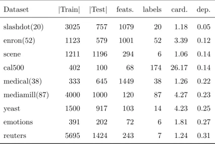
Table 2: Summary of benchmark datasets. For each dataset the dependency measured using (18) is reported in the last column. The datasets are sorted by this value in ascending order
Dataset |Train| |Test| feats. labels card. dep.
slashdot(20) 3025 757 1079 20 1.18 0.05 enron(52) 1123 579 1001 52 3.39 0.12 scene 1211 1196 294 6 1.06 0.14 cal500 402 100 68 174 26.17 0.14 medical(38) 333 645 1449 38 1.26 0.22 mediamill(87) 4000 1000 120 87 4.27 0.23 yeast 1500 917 103 14 4.23 0.25 emotions 391 202 72 6 1.81 0.27 reuters 5695 1424 243 7 1.24 0.31 parameters.
Table 3 reports the Hamming scores obtained by all the algorithms over
the benchmark datasets. At first glance, their results are quite similar for all
of them, except CC. In fact, comparing their scores by means of a
Friedman-Nemenyi test [7] the differences between BR, M3LI, M3Lρ, SVM⊗I and SVM⊗ρ are not significant at all. We do think that this fact makes sense considering the
properties of the algorithms compared and the characteristics of the benchmark
datasets used in the experiments. In this kind of experiment, which combines datasets with low and high label dependence, it would be abnormal that one
of the methods outperforms the rest. The reason is that some of the methods
are well suited for those tasks in which the labels tend to be independent (BR,
M3LI and SVM⊗I), other for domains in which the labels show unconditional label dependence (M3Lρ and SVM⊗ρ) and the last method (CC) for datasets with conditional label dependence. Thus, it is logical that none of the methods
statistically outperforms the rest for all datasets. Each method should perform
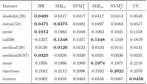
Table 3: Average Hamming scores achieved by SVM⊗, M3L, BR and CC. SVM⊗, M3L both used without and with the correlation matrix on real world datasets. The score of the best method for each dataset is shown in bold
Dataset BR M3LI SVM⊗I M3Lρ SVM⊗ρ CC slashdot(20) 0.0400 0.0417 0.0417 0.0417 0.0414 0.0548 enron(52) 0.0475 0.0475 0.0481 0.0497 0.0483 0.0517 scene 0.1012 0.1063 0.1048 0.1062 0.1045 0.1158 cal500 0.1357 0.1348 0.1357 0.1348 0.1349 0.1819 medical(38) 0.0130 0.0126 0.0133 0.0133 0.0141 0.0131 mediamill(87) 0.0325 0.0330 0.0330 0.0331 0.0330 0.0335 yeast 0.1995 0.1990 0.1989 0.1974 0.1975 0.2110 emotions 0.2162 0.2112 0.2096 0.2162 0.2021 0.2376 reuters 0.0462 0.0458 0.0463 0.0456 0.0467 0.0450
Therefore, the Hamming scores reported must be analyzed taking into
ac-count the level of dependency of each dataset. Interestingly, the conclusions of
such analysis are in line with the expected behavior of each method. It seems
that when label dependence is very low BR performs better than the rest of the
methods. For instance, in the three datasets with lowest label dependence (
en-ron,scene andslashdot) the winner is BR. But when label dependence starts to
increase, other methods take the lead. And particularly when the label depen-dence is high, the performance of M3Lρ and SVM⊗ρ is better. It is worth noting that M3Lρ and/or SVM⊗ρ outperform BR in the three datasets with largest la-bel dependence (emotions,reutersandyeast). In the case ofreutersdataset the
absolute winner is CC, a method that performs poorly for most of the datasets.
This seems to suggest that there is some level of conditional label dependence
in such dataset.
Thus, these results are promising but do not totally support (statistically)
favorable to the versions using the correlation kernel when the dependency is
large. On the other hand, these results may not be conclusive since the number
of datasets was rather low to generalize the behavior of the algorithms. A larger collection of datasets, with different degrees of label dependence, would
be needed.
6.2. Performance on Synthetic Multilabel Classification Tasks
In order to elucidate the relation between the unconditional dependence and the performance of SVM⊗
ρ and M3Lρ we generated a collection of synthetic datasets of different sizes and degrees of dependency. For this purpose, we used
a synthetic dataset generator [16] based on a genetic algorithm to obtain ML
datasets with specific characteristics. The aim of the generator was to produce
a dataset with a givencardinalityanddependency.
We built 108 datasets (each one composed by a training, a validation and
a testing set) by varying four parameters. In all cases the input space was
Rp+1 with p ∈ {10,25,50,100}, see (14). The size m of the set of labels
var-ied in {100,150,200}. The target cardinalities (average number of labels per example) ranged in{2.5,3.5,4.5}. The desired values for dependency were in [0.05..0.65]. The generator draws a set of 400 points in [0,1]p that will be used to build the training set. Then, it searches formhyperplanes such that the set of labels so obtained fits as much as possible the cardinality and dependency
required. Notice that it is nearly impossible to obtain a dataset fulfilling some
combinations of these parameters. Thus, it can only obtains an approximate
solution. After obtaining those hyperplanes, the validation and testing sets are
generated with 400 and 600 examples respectively.
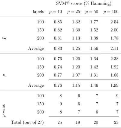
We used these synthetic datasets to check the performance of SVM⊗I and M3LIwith respect to the versions using the correlation kernel, SVM⊗ρ and M3Lρ. After adjusting theCparameter using train and validation sets, the performance was computed on the test set. In this case, C ranged in{10i:i=−1,0,1,2,3}. We show the average Hamming scores achieved by SVM⊗ρ and SVM⊗I in Table 4 and Figure 1, where the datasets are grouped by the number of labels
Table 4: Average Hamming scores (expressed as percentages) achieved by SVM⊗usingIand
ρmatrices for different number of labels and dimensions (p) of the input space. Each score
is the average of 9 datasets. The last band shows the number of times that the correlation
kernel helps to improve the performance of the algorithm SVM⊗
SVM⊗ scores (% Hamming) labels p= 10 p= 25 p= 50 p= 100 I 100 0.85 1.32 1.77 2.54 150 0.82 1.30 1.52 2.00 200 0.81 1.13 1.38 1.78 Average 0.83 1.25 1.56 2.11 ρ 100 0.76 1.20 1.64 2.38 150 0.74 1.20 1.42 1.92 200 0.77 1.07 1.31 1.68 Average 0.76 1.15 1.46 1.99 ρ wins 100 8 6 7 9 150 9 6 7 7 200 8 7 6 7 Total (out of 27) 25 19 20 23
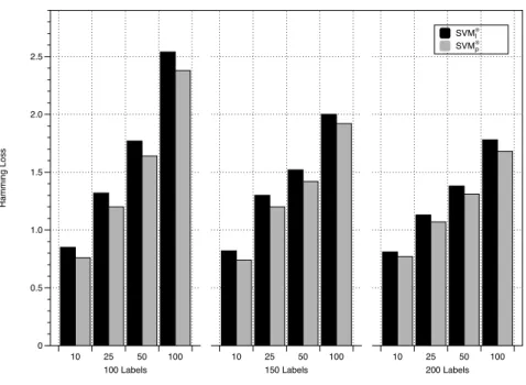
SVM⊗ I SVM⊗ ρ H a mmi n g L o ss 0 0.5 1.0 1.5 2.0 2.5 100 Labels 10 25 50 100 150 Labels 10 25 50 100 200 Labels 10 25 50 100
Figure 1: SVM⊗ρ and SVM⊗I average Hamming scores over artificial datasets when the number
of labels varies (100,150 and 200). For each case, four different dimensions (10, 25, 50 and 100) of the input space were analyzed. The scores are expressed as percentages
(m) and input space dimension (p). In general, we observe that the use of the correlation kernel (17) improves the performance when m and pincrease. This is shown in the last band of Table 4, which reveals the number of times the version using the correlation kernel wins over the version using the identity
matrix. As we can observe, SVM⊗ρ outperforms SVM⊗I for every combination of the parameters studied. In fact, SVM⊗ρ wins in 87 cases out of 108. Moreover, it seems that the differences between both are greater in favor of SVM⊗ρ when the learning tasks become harder, when the size of the input space and the number
of labels increase. In such cases, the role played by correlations appears to be
decisive.
But we also need to study these results taken into account the level of
un-conditional dependence present. The advantage of using the correlation kernel
SVM⊗ I− SVM⊗ ρ Fit H a mmi n g L o ss D iff e re n ce (SVM ⊗−I SVM ⊗)ρ −0.10 −0.05 0 0.05 0.10 0.15 0.20 0.25 0.30 0.35 0.40 0.45 Dependency 0 0.05 0.10 0.15 0.20 0.25 0.30 0.35 0.40 0.45 0.50 0.55 0.60 0.65 0.70
Figure 2: SVM⊗ρ vs. SVM⊗I. For each synthetic dataset we represent a point whose X
coordinate is the dependency of the training set and whose Y coordinate represents the benefit of using the correlation kernel in terms of Hamming score
which depict the increase in performance (difference between Hamming scores)
obtained when using the correlation kernel with respect to the use of the identity
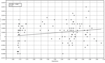
matrix for both SVM⊗ and M3L, respectively. For instance, in Figure 2 we can observe that when unconditional dependence is low, it seems that SVM⊗I per-forms slightly better that SVM⊗ρ. But, when the dependency increases, SVM⊗ρ is the clear winner. A similar behavior happens in the case of M3L, see Figure 3.
These pictures show that the benefits of using the matrixρincrease proportion-ally to the dependency. In Figure 4 we compared M3Lρ and SVM⊗ρ and we can observe that the performance of the latter is better than the former and that
the difference between both algorithms increases with the dependency too.
To statistically confirm these conclusions, we compare M3LI, M3Lρ, SVM⊗I and SVM⊗ρ by means of a Friedman-Nemenyi test [7] on the scores obtained over the synthetic datasets. The test, which is graphically summarized in Figure 5,
found significant differences between using or not the correlation kernel both
for SVM⊗ and for M3L. It also found that our approach SVM⊗ρ is significantly better than the rest of algorithms, although the differences were small. In
M3LI − M3Lρ Fit H a mmi n g L o ss D iff e re n ce (M3 L I − M3 L ρ ) −0.15 −0.10 −0.05 0 0.05 0.10 0.15 0.20 0.25 0.30 0.35 0.40 0.45 Dependency 0 0.05 0.10 0.15 0.20 0.25 0.30 0.35 0.40 0.45 0.50 0.55 0.60 0.65 0.70
Figure 3: M3Lρvs. M3LI. For each synthetic dataset we represent a point whose X coordinate
is the dependency of the training set and whose Y coordinate represents the benefit of using the correlation kernel in terms of Hamming score
addition, we performed a Wilcoxon signed-rank test between SVM⊗ρ and M3Lρ, obtaining that the difference is significant withp <0.01 in favor of our approach.
7. Conclusions
This paper presents a new kernel-based approach to handle ML classification
tasks when the aim is to optimize a loss function defined by micro-averaging a
measure based on labels. The core idea is to transform a ML task into a binary
classification problem whose inputs are drawn from a tensor space of the original
input space and a representation of the labels. In fact, the goal is to exploit
the correlation between the labels because they are normally not assigned
in-dependently of each other; instead, they present statistical dependencies. From
a learning point of view, these relationships constitute a crucial source of in-formation, in addition to that coming from the mere description of the objects.
Here, we propose tensor kernels for combining both sources of information, and
a correlation kernel for taking advantage of such label correlations.
ben-M3LP − SVM⊗ ρ Fit H a mmi n g L o ss D iff e re n ce (M3 L P − SVM ⊗)ρ −0.0010 −0.0008 −0.0006 −0.0004 −0.0002 0 0.0002 0.0004 0.0006 0.0008 0.0010 0.0012 0.0014 0.0016 Dependency 0 0.05 0.10 0.15 0.20 0.25 0.30 0.35 0.40 0.45 0.50 0.55 0.60 0.65 0.70
Figure 4: SVM⊗ρ vs. M3Lρ. For each synthetic dataset we represent a point whose X
coordi-nate is the dependency of the training set and whose Y coordicoordi-nate represents the benefit of using the correlation kernel in terms of Hamming score
efit form capturing unconditional label dependence. Even in the case of
Ham-ming loss, which theoretically can be optimized assuHam-ming independence between
labels, like BR does, our method can improve such performance when the
un-conditional dependence increases. This is a quite interesting result because it
answers the questions raised in [6] whether exploiting label dependence could
help to improve Hamming loss performance. In their discussion, they conclude
that the improvements obtained by some ML classifiers (Probabilistic
Classi-fier Chains in their case) are due to employ a much richer hypothesis space in comparison to the one used by BR. Here, our approach enriches its
hypoth-esis space by considering label correlations through a kernel and outperforms
those methods that assume label independence whenever such correlations are
present.
Acknowledgments
The research reported here is supported in part under grant TIN2011-23558
from the MICINN (Ministerio de Econom´ıa y Competitividad, Spain). We
Figure 5: Results of a Friedman-Nemenyi test (confidence level of 95%) using the scores
obtained by SVM⊗I, SVM⊗ρ, M3LI and M3Lρ. The scale from 1 to 4 shows the average
rank of each method regarding its performance. The bold line links those algorithms whose differences in performance are not statistically significant
datasets and software used in this paper, as well as the anonymous reviewers who undoubtedly contributed to improve the quality of this paper.
References
[1] C.C. Chang, C.J. Lin, LIBSVM: A library for support vector machines, ACM Transactions on Intelligent Systems and Technology 2 (2011) 27:1–
27:27.
[2] W. Cheng, E. H¨ullermeier, Combining instance-based learning and logistic
regression for multilabel classification, Machine Learning 76 (2009) 211–
225.
[3] K. Dembczy´nski, W. Cheng, E. H¨ullermeier, Bayes optimal multilabel
clas-sification via probabilistic classifier chains, Proceedings of the 27th
Inter-national Conference on Machine Learning (ICML) (2010).
[4] K. Dembczy´nski, W. Waegeman, W. Cheng, E. H¨ullermeier, An exact al-gorithm for f-measure maximization, in: Proceedings of the Neural
[5] K. Dembczy´nski, W. Waegeman, W. Cheng, E. H¨ullermeier, On label
dependence and loss minimization in multi-label classification, Machine
Learning 88 (2012) 5–45.
[6] K. Dembczy´nski, W. Waegeman, E. H¨ullermeier, An analysis of chaining
in multi-label classification, in: ECAI 2012, pp. 294–299.
[7] J. Demˇsar, Statistical Comparisons of Classifiers over Multiple Data Sets,
Journal of Machine Learning Research 7 (2006) 1–30.
[8] J.R. Doppa, J. Yu, C. Ma, A. Fern, P. Tadepalli, Hc-search for multi-label
prediction: An empirical study, in: Proceedings of AAAI Conference on
Artificial Intelligence (AAAI).
[9] A. Elisseeff, J. Weston, A kernel method for multi-labelled classification,
in: In Advances in Neural Information Processing Systems 14, MIT Press,
2001, pp. 681–687.
[10] D. Hardoon, J. Shawe-Taylor, Decomposing the tensor kernel support
vec-tor machine for neuroscience data with structured labels, Machine learning
79 (2010) 29–46.
[11] B. Hariharan, S. Vishwanathan, M. Varma, Efficient max-margin
multi-label classification with applications to zero-shot learning, Machine
Learn-ing 88 (2012) 127–155.
[12] T. Joachims, T. Finley, C. Yu, Cutting-plane training of structural svms,
Machine Learning 77 (2009) 27–59.
[13] A. Kumar, S. Vembu, A.K. Menon, C. Elkan, Beam search algorithms for
multilabel learning, Mach. Learn. 92 (2013) 65–89.
[14] P. Li, H. Li, M. Wu, Multi-label ensemble based on variable pairwise
con-straint projection, Information Sciences 222 (2013) 269 – 281.
[15] H. Liu, S. Zhang, X. Wu, Mlslr: Multilabel learning via sparse logistic
[16] ´O. Luaces, J. D´ıez, J. Barranquero, J.J. del Coz, A. Bahamonde, Binary
relevance efficacy for multilabel classification, Progress in Artificial
Intelli-gence 4 (2012) 303–313.
[17] E. Monta˜n´es, R. Senge, J. Barranquero, J. Quevedo, J.J. del Coz,
E. H¨ullermeier, Dependent binary relevance models for multi-label
clas-sification, Pattern Recognition 47 (2014) 1494 – 1508.
[18] E. Monta˜n´es, J.R. Quevedo, J.J. del Coz, Aggregating independent and
dependent models to learn multi-label classifiers, Machine Learning and
Knowledge Discovery in Databases (2011) 484–500.
[19] J. Petterson, T. Caetano, Reverse multi-label learning, Advances in Neural
Information Processing Systems 23 (2010) 1912—1920.
[20] J.R. Quevedo, O. Luaces, A. Bahamonde, Multilabel classifiers with a
prob-abilistic thresholding strategy, Pattern Recognition 45 (2012) 876–883.
[21] J. Read, L. Martino, D. Luengo, Efficient monte carlo methods for
multi-dimensional learning with classifier chains, Pattern Recognition 47 (2014)
1535 – 1546.
[22] J. Read, L. Martino, P.M. Olmos, D. Luengo, Scalable multi-output label
prediction: From classifier chains to classifier trellises, Pattern Recognition
48 (2015) 2096–2109.
[23] J. Read, B. Pfahringer, G. Holmes, E. Frank, Classifier chains for multi-label classification, Machine Learning 85 (2011) 333–359.
[24] R. Schapire, Y. Singer, Boostexter: A boosting-based system for text
cat-egorization, Machine learning 39 (2000) 135–168.
[25] S. Szedm´ak, J. Shawe-Taylor, E. Parrado-Hern´andez, Learning via linear
operators: Maximum margin regression; multiclass and multiview learning
at one-class complexity, Technical Report, PASCAL, Southampton, UK.,
[26] I. Tsochantaridis, T. Joachims, T. Hofmann, Y. Altun, Large margin
meth-ods for structured and interdependent output variables, Journal of Machine
Learning Research 6 (2006) 1453.
[27] G. Tsoumakas, I. Katakis, Multi Label Classification: An Overview,
Inter-national Journal of Data Warehousing and Mining 3 (2007) 1–13.
[28] G. Tsoumakas, I. Katakis, I. Vlahavas, Mining Multilabel Data, In O.
Mai-mon and L. Rokach (Ed.), Data Mining and Knowledge Discovery
Hand-book, Springer (2010).
[29] G. Tsoumakas, I. Katakis, I. Vlahavas, Random k-Labelsets for
Multi-Label Classification, IEEE Transactions on Knowledge Discovery and Data
Engineering (2010).
[30] G.T. Tsoumakas, E. Spyromitros-Xioufis, J. Vilcek, I. Vlahavas, Mulan: A
Java library for multi-label learning, Journal of Machine Learning Research
12 (2011) 2411–2414.
[31] J. Weston, B. Sch¨olkopf, O. Bousquet, Joint kernel maps, Computational
Intelligence and Bioinspired Systems (2005) 135–168.
[32] J. Yu, Y. Rui, Y.Y. Tang, D. Tao, High-order distance-based multiview
stochastic learning in image classification, Cybernetics, IEEE Transactions
on 44 (2014) 2431–2442.
[33] M.L. Zhang, J.M. Pe˜na, V. Robles, Feature selection for multi-label naive bayes classification, Information Sciences 179 (2009) 3218–3229.
[34] M.L. Zhang, Z. Zhou, ML-KNN: A Lazy Learning Approach to Multi-label
Learning, Pattern Recognition 40 (2007) 2038–2048.
[35] Z. Zhou, Learning And Mining from DatA (LAMDA).