w o r k i n g
p
a
p
e
r
11
23R
The Impact of Vacant, Tax-Delinquent,
and Foreclosed Property on
Sales Prices of Neighboring Homes
Working papers
of the Federal Reserve Bank of Cleveland are preliminary materials circulated to
stimulate discussion and critical comment on research in progress. They may not have been subject to the
formal editorial review accorded offi cial Federal Reserve Bank of Cleveland publications. The views stated
herein are those of the authors and are not necessarily those of the Federal Reserve Bank of Cleveland or of
the Board of Governors of the Federal Reserve System.
Working Paper 11-23R
March 2012*
The Impact of Vacant, Tax-Delinquent, and Foreclosed Property on
Sales Prices of Neighboring Homes
by
Stephan Whitaker and Thomas J. Fitzpatrick IVIn this empirical analysis, we estimate the impact of vacancy, neglect
associ-ated with property-tax delinquency, and foreclosures on the value of neighboring
homes using parcel-level observations. Numerous studies have estimated the
impact of foreclosures on neighboring properties, and these papers theorize that
the foreclosure impact works partially through creating vacant and neglected
homes. To our knowledge, this is only the second attempt to estimate the impact
of vacancy itself and the fi rst to estimate the impact of tax-delinquent properties
on neighboring home sales. We link vacancy observations from Postal Service
data with property-tax delinquency and sales data from Cuyahoga County (the
county encompassing Cleveland, Ohio). We estimate hedonic price models with
corrections for spatial autocorrelation. We fi nd that an additional property within
500 feet that is vacant, delinquent, or both reduces the home’s selling price by at
least 1.3 percent. In low-poverty areas, tax-current foreclosed homes have large
negative impacts of 4.6 percent. In high-poverty areas, we observe positive
cor-relations of sale prices with tax-current foreclosures and negative corcor-relations
with tax-delinquent foreclosures. This may refl ect selective foreclosing on
better-maintained properties or better maintenance by tax-paying foreclosure auction
winners. The marginal medium-poverty census tracts display the largest negative
responses to vacancy and delinquency in nearby nonforeclosed homes.
JEL Codes: R31, R32, R38, R58, C31, R23.
Keywords: foreclosure, vacancy, abandonment, residential property, home prices,
spatial modeling, low-value property, distressed property.
*Originally posted in September 2011. First revision December 2011.
Stephan Whitaker is at the Federal Reserve Bank of Cleveland and he can be reached at 216-579-2040 or stephan.whitaker@clev.frb.org. Thomas J. Fitzpatrick IV is at the Federal Reserve Bank of Cleveland and he can be reached at 216-579-3087 or thomas.j.fi tzpatrick@clev.frb.org. The authors would like to thank Mary Zenker for her extensive research assistance on this proj-ect and Kyle Fee and Carole Ouedraogo for their additional help. They are grateful to Michael Schramm for bringing the vacancy data to their attention and to Lisa Nelson for sharing her list of institutional market participants. They also appreciate all the useful comments they received from
1
Introduction
Recent events in housing markets are attracting much scholarly attention to foreclosures. One line of research that is developing rapidly focuses on the externalities associated with foreclosure, primarily a foreclosed home’s impact on surrounding properties. There are two general deficiencies with this line of research: the nearly exclusive focus on robust housing markets, and the assumption that foreclosures themselves, rather than factors correlated with foreclosure, drive down surrounding housing prices. This paper attempts to fill the gaps in prior research in two ways. First, it focuses upon a less robust housing market: Cuyahoga County, Ohio (home to Cleveland). Second, it incorporates parcel-level vacancy and real property tax delinquency (as a measure of neglect) in addition to foreclosure. We are able to estimate the impact of vacant and tax-delinquent homes on neighboring properties and correct the estimates of the impact of foreclosures by directly controlling for nearby vacant and tax-delinquent homes. We demonstrate important differences in the impact of foreclosure in different submarkets. In high poverty areas, we find evidence of selective foreclosure in a positive relationship between tax-current foreclosure and neighboring home sales. Pooling these high-poverty observations with medium and low-poverty observations obscures the large negative impact of foreclosures that is measurable in mid-to-upper income areas. Finally, we are able to use the coincidence of vacancy, delinquency, and foreclosure as a measure of abandoned properties. This measure enables us to estimate of their impact on home values.
Foreclosure, vacancy, and tax delinquency differ in important ways, though they may all lower surrounding home values or indicate distress that lowers home values. Foreclosure occurs when a debtor fails to pay a debt secured by the debtor’s home, and the creditor opts to seize and sell the property instead of continuing to seek payment from the debtor. During foreclosure, homeowners have little incentive to maintain their homes, as every dollar put into upkeep or
improvements will primarily benefit the foreclosing lender.1 Thus, recently foreclosed homes are
more likely to be distressed due to deferred maintenance than homes that have not recently been through a foreclosure. Additionally, foreclosure adds a unit of supply to a local housing market. Assuming a competitive housing market, this additional supply should put downward pressure on home values. Finally, foreclosure may lower surrounding home values when they are used as comparable properties by real estate appraisers or realtors to price non-foreclosed real estate. In light of the volume of properties recently moving through REO (real estate owned), lenders lower the sales prices of homes they own in order to sell them quickly, because the carrying costs of vacant properties are high. When appraisers or realtors determine the value of a home, they may select foreclosed homes as comparable properties without considering the eagerness of the seller.2
Vacancy is closely related to foreclosure, but distinct in important ways. A home that has been foreclosed upon will be vacant immediately after the foreclosure but the vacancy may be temporary, as the property is auctioned off to a new owner or to a bank or investor who usually attempts to find a new owner.3 Vacancy is distinct from foreclosure in that a property is vacant when it is not
being occupied, which is not a result of a foreclosure in the vast majority of cases (there are seven 1In states that allow deficiency judgments, where the lender can pursue borrowers for the difference between the
amount owed on the loan and the price paid for the home at foreclosure auction, homeowners may have more of an incentive to actively maintain homes. Historically, however, deficiency judgments are not commonly pursued for many reasons. For example, homeowners who have gone through foreclosure rarely have the ability to repay a deficiency judgment, and such judgments are more easily dischargeable in bankruptcy than secured debt.
2Real estate appraisal guidelines allow for some discretion when selecting comparable properties. See,
e.g. Uniform Standards of Professional Appraisal Practice 2010-2011, Standards 1 & 2, available at http://www.uspap.org/USPAP/frwrd/uspap toc.htm. Thus, foreclosure liquidations and REO sales may not be used when selecting comparable properties.
3Not all purchasers at foreclosure auctions seek to quickly fill the home. Some spend time rehabilitating it or
marketing it to other property investors (Ergungor and Fitzpatrick 2011). Some homes remain vacant for years after a foreclosure, especially high-poverty areas (Whitaker 2011).
times more vacancies than foreclosures in our data).4 Vacancy lowers surrounding property values
in ways that closely resemble foreclosure. Each vacancy is another likely unit of supply on the market, which should put downward pressure on home values. Vacant properties are usually not maintained as well as occupied properties because no one is present on a daily basis to care for them. While they may be cared for by an owner living elsewhere, there is less incentive and opportunity to maintain them as often and as carefully as an owner-occupier would. This problem is exacerbated with long-term vacancy, which occurs naturally in less robust housing markets where there may not be sufficient demand to reoccupy vacant houses, and in colder-weather climates where a single winter can cause significant damage to a property that is not attentively maintained.
While vacancy and foreclosure intuitively put downward pressure on home values through supply and disamenity channels, real property-tax delinquency does not: it neither immediately creates additional supply nor is it easily observable by neighborhood residents.5 Yet, certain levels of
tax delinquency may signal the abandonment of property by its owner, because once a property becomes tax delinquent it may be taken from the owner through tax foreclosure. Property is abandoned at the point that property owners and inhabitants stop investing in the property with the intent of foregoing their ownership interests. Abandonment usually occurs when a property’s carrying, operating, or rehabilitation costs are too high relative to the property’s value. The condition of abandoned property deteriorates rapidly, as there is no one maintaining or improving it. The decision to abandon property is made subjectively, and cannot be directly observed. This has led previous researchers to use subjective municipal determinations of whether a property 4We consider a property vacant if it is not legally occupied. In some sense this may over-count vacancies, as some
may be occupied by squatters. But such occupants have little incentive to maintain, and virtually no incentive to improve, the property.
5A tax delinquency becomes a unit of supply if it is eventually subject to tax foreclosure. A tax-delinquent home
has been abandoned (Mikelbank 2008). While the subjective assessments are not reproducible, these studies show that when the impact of foreclosed property on surrounding home values is not considered alongside vacant and abandoned property, it overstates the impact of foreclosure. We use combinations of reproducible, objective indicators as proxies for abandonment. If we find these indicators are informative, they may be a substitute for this difficult-to-measure status.
In the years following the rapid decline in housing values, hedonic price modeling has been applied to evaluate the impact of properties that have been through a foreclosure. Foreclosure sales are easily identified in county recorder or court records, so many studies have been conducted on the impact of foreclosures. Often these studies are motivated by suggesting the foreclosed properties are frequently vacant, abandoned, and blighted. However, foreclosure is a very noisy measure of the impact of vacancy and abandonment. A few of the studies have incorporated the impact of vacancy and abandonment, but this has been limited by the unavailability of parcel-level vacancy data (Mikelbank 2008, Hartley 2010). With data on vacancy, foreclosure, and tax-delinquency, we can begin to disentangle the impact of each status on the value of neighboring properties.
In order to better understand these dynamics, this analysis is the first application of hedonic price modeling to a panel data set, specifically representing vacancy and property-tax delinquency of residential properties. To the authors’ knowledge, this is the first study to use property-tax delinquency as an objective indicator of abandonment. This study is the first to use the U.S. Postal Service’s (USPS) administrative records of vacancy to identify vacant properties at the address level. The records are commercially available on a monthly basis, so homes can be observed moving into and out of vacancy. Also, the time variation in the data gives us both increased accuracy in the count of nearby vacant homes at the time of the sale, and it creates additional variation in the vacancy counts within neighborhoods. Focusing on within-neighborhood variation addresses some of the endogeneity issues that always challenge hedonic price analyses. We find that when
foreclosure, vacancy, and property-tax delinquency are all included, the impact of foreclosure on surrounding home values is reduced.
The rest of the paper proceeds in five sections. In the remainder of this section we review the relevant literature. In section two, we discuss the theory behind our modeling. In section three we discuss the data we use and provide descriptive statistics. In section four we discuss our results, and in section five we conclude and discuss policy implications of our findings.
1.1 Literature
Since housing prices cooled in 2007, policymakers are increasingly aware of the external costs of foreclosure, vacancy, and abandonment. Research has intensified over the past few years, but it primarily focuses upon foreclosure. While foreclosure may lower surrounding home values, vacancy and abandonment have long been recognized by practitioners as more important roadblocks to revitalizing distressed neighborhoods. Interest in vacancy and abandonment dates to well before the current crisis. For example, one early paper developed a theoretical model based upon New York City housing markets that approximated that owners would abandon property when the current level of rents in the neighborhood did not justify the rebuilding or renovation of a distressed property (White 1986). Yet this research has rarely made an attempt to quantify the impact of vacancy and abandonment on surrounding home values.
One gap in research on abandoned properties is the lack of a universal definition of “abandon-ment.” Municipalities tend to use a period of vacancy as a proxy for abandoned structures, but the period they must be vacant to become abandoned varies widely (Pagano and Bowman 2000). A structure is generally considered abandoned when it is chronically vacant, uninhabitable, and the owner is taking no steps to improve the property (Cohen 2001). Unfortunately, to determine that a property is uninhabitable or in disrepair researchers rely upon an assessment from the municipality
itself, obtained through inspections (Cohen 2001, Mikelbank 2008). This data is often incomplete, because municipalities lack the resources to frequently survey all properties within their jurisdic-tion (Pagano and Bowman 2000). These inconsistent definijurisdic-tions make it impossible to accurately compare results across cities.
For the purposes of this study, we use vacancy, tax delinquency, and their coincidence as measures of distress and abandonment. Vacancy is nearly universal among abandoned properties, as by definition they are not being cared for by either owners or inhabitants. Tax delinquency has been referred to as “the most significant common denominator among vacant and abandoned properties,” (Alexander 2005), and correlations exist between tax-delinquency rates and decreases in home sales prices (Simons, Quercia, and Maric 1998). This is logical, as owners who plan to retain ownership either pay property taxes or run the risk of losing the property in a tax foreclosure. Property owners with no interest in retaining ownership have no incentive to pay property taxes. Owners with no interest in retaining ownership also have no incentive to maintain their property, so where we find property tax delinquency, we would expect to find deferred maintenance.
Research ties widespread vacancy and abandonment to long-term population decline. The pro-cess of filtering, where the occupation of new, high quality residential construction results in old, low-quality residential vacancies has been analyzed for decades (Lowry 1960). Cities that self-report the largest supply of abandoned housing have experienced persistent population loss, suggesting that abandonment occurs in the later stages of a neighborhood’s lifecycle (Cohen 2001). When building permits outpace household growth in a metropolitan area, filtering causes increased va-cancy and abandonment in the city’s urban core and inner-ring suburbs (Bier and Post 2003). The durable nature of housing results in a very slow adjustment of the housing stock to match the smaller population (Glaeser and Gyourko 2005). The lag manifests itself in vacancy and abandon-ment. Abandoned property is a significant, long-term problem in older industrial cities that have
experienced outmigration from their urban cores, but such filtering also leads to some abandonment in cities with generally robust housing markets.
Until recently, most research on the impact of urban decline has focused on foreclosures in robust housing markets. The most commonly cited study on the topic estimates that each mortgage foreclosure within one eighth of a mile (660 feet) of a single-family home lowered its value by about one percent, based on one year of home sales data from Chicago in the late 1990s (Immergluck and Smith 2006). In order to determine whether foreclosures create significant price declines to surrounding property or are simply a result of local housing trends, Harding, Rosenblatt and Yao examine the impact of nearby foreclosures on home sales in select zip codes across seven metropolitan areas over nearly 20 years, and factor in local price trends (2009).6 They find that above local housing price trends, each foreclosure within 300 feet lowers a home’s value by up to one percent, and each foreclosure from 300-500 feet lowers a home’s value by about one half of one percent.
Schuetz, Been, and Ellen control for home prices prior to foreclosures and investigate the lin-earity of the relationship between the number of foreclosures and price discount on surrounding homes (2008). Using data from New York City from multiple years, they find that foreclosures within 250 feet of a home reduce its value by one to two percent. Outside of the 250 foot ring, a larger number of foreclosures is necessary to impact a home’s value: three or more from 250-500 feet lowers a home’s value by one to three percent, and six or more from 500-1000 feet lower a home’s value by about three percent.
Campbell, Giglio, and Pathak look more broadly at the impact of forced sales on home prices (2011). They define forced sales as those resulting from bankruptcy, death, and foreclosure. Looking at housing data for Massachusetts over 20 years, they find that forced sales due to foreclosure have
much steeper price discounts than those due to bankruptcy or death. Controlling for the average level of voluntary sales prices, they find that a foreclosure within a twentieth of a mile (264 feet) lowers the value of a home by about 1 percent, and the closer the foreclosure to the home the larger the discount.
Lin, Rosenblatt, and Yao (2009) attempt to better understand why foreclosures lower surround-ing home values. They used a theoretical model for home pricsurround-ing ussurround-ing comparable properties, attempting to reproduce the effects of appraisers and realtors. They estimated that in Chicago, each foreclosure liquidation can depress short-run property values of homes within a half mile as much as 8.7 percent in down markets and 5 percent in up markets.7
Three foreclosure studies have been published making use of transaction and property char-acteristics data from the suburban county adjacent to St. Louis, Missouri (Rogers and Winter 2009, Rogers 2010, Groves and Rogers 2011). Rogers and Winter find evidence that the marginal impact of foreclosure declines with distance from the foreclosure, time since the sheriff sale, and the prevailing foreclosure rate (2009). Rogers’ data reaches back to the years from 2000 to 2005, when foreclosures where far less common and exhibited larger impacts. A second study presents evidence that comparable marginal impacts were stronger in the earlier years of the data than in the later years (Rogers 2010). Most of the estimates are less than one percent per unit when measured at distances and time comparable to other studies, such as 200 yards and twelve months. The final study examines the ability of restrictive covenants to mitigate the externalities of foreclosures (Groves and Rogers 2011).
Only two studies look beyond foreclosure and incorporate vacancy into their analysis (Mikelbank 2008, Hartley 2010). One uses vacancy rates to classify neighborhoods into broad categories. 7This model assumed that foreclosure liquidations of comparable properties are used by realtors when pricing a
home. Anecdotally, realtors and appraisers in less robust housing markets report ignoring foreclosure liquidations when pricing comparable properties unless there are no other reasonable comparisons.
Hartley attempts to delineate between the “supply” and “disamenity” effects of foreclosures to determine how much of the price discount was due to each (2010). By looking at different types of foreclosed property in Chicago, Hartley decomposes the effects of foreclosure on nearby housing in census tracts with low and high vacancy rates. The explicit assumption in Hartley’s work is that occupied multi-family buildings are not substitutes for single-family homes, so a renter-occupied multi-family building foreclosure will not change the potential housing supply for persons seeking a single-family home, and vice versa. In census tracts with low vacancy rates, he finds that each foreclosed single-family home within 250 feet reduces a home’s value by 1.6 percent due to an increase in supply, while the disamenity effect of the foreclosed multifamily buildings is near zero. In census tracts with high vacancy rates, he estimates the disamenity effect of a foreclosed multi-family home lowers surrounding single-family property values by about two percent, while the supply effect is near zero.
One issue common to all of these studies is that they all acknowledge that foreclosures likely lower surrounding home values by becoming disamenities or adding supply to the market, but fail to distinguish between foreclosures that are reoccupied quickly, foreclosures that sit vacant and are well maintained, and those that become abandoned. Hartley’s results hint at the importance of this distinction by illustrating that neighborhood property values are lowered due to supply or disamenity, depending on the location (and likely the condition) of the property. Understanding the difference between foreclosed, vacant, and abandoned property is critical for policymakers who seek to understand how to address these issues. Mikelbank illustrates that estimating the impact of either vacant and abandoned property or residential foreclosures in isolation overstates the impact of both, based upon his empirical analysis of one year of housing sales in Columbus, Ohio (2008). In this paper, we build on the previous studies, focusing on the housing transactions in Cuyahoga County, Ohio, in an attempt to better understand the interplay between foreclosures, vacancies,
abandoned properties and surrounding home values.
2
Theory
The methods we will employ are based in the field of hedonic models of real estate pricing. Orig-ination of these models is generally credited to Rosen (1974). In their simplest application, the sales price of a home is regressed on indicators of the home’s characteristics, and the coefficients are interpreted as the marginal prices of those characteristics (see equation 1). Pi is a home sale price. zij are characteristics of the home and its location.
Pi = α+
J
X
j=1
βjzij +εi (1)
The HP model relies on some standard assumptions which, nevertheless, could be violated in reality. It assumes the housing market is competitive and that both buyers and sellers are fully informed.8 Using a linear specification suggests that the characteristics of the home can be costlessly
repackaged. This is obviously not the case, so most applications employ a semi-log specification that implicitly interacts all the characteristic measures. In this specification, the coefficients are not interpreted as prices, but rather percentage changes in the price.
ln(Pi) = α+ J
X
j=1
βjzij +εi (2)
Despite including a set of measures of the area surrounding an observed house sale, researchers generally suspect that there are important unobserved location factors. These include amenities and disamenities the researchers has not controlled for (the possibilities are endless). The impact of these factors is also thought to vary with distance. A home closer to the amenity or disamenity 8A significant number of homes in Cuyahoga County have been purchased by out-of-state investors over the
internet. Homes are also purchased out of REO inventory blindly as part of a bulk sale at a pre-negotiated price. Full information is doubtful in these cases.
will have a larger price response. Omitting a distance-weighted indicator of the factor leaves its influence in the error term. Equation 3 is a hedonic price model that gives two options to address this (Anselin 1988).
P = λW1P+ZB+ε (3)
ε = ρW2ε+µ (4)
µ ∼ N(0, σ2I) (5)
Equations 1 and 2 used summation notation to emphasize the contribution of multiple character-istics to the sale price. We switch to matrix notation (following the literature) here because the spatial models center on a spatial weight matrix. W1 is a spatial weighting matrix that gives large weight to the prices of nearby homes and small weight to the prices of far away homes. Multiplying the price vector (P) byW1 creates a vector of weighted averages of nearby home prices. Including
these averages as a control removes the gradient between high-price and low-price neighborhoods.9
The remaining variation within neighborhoods tells us approximately how much sale prices would change if we could add or remove distressed properties. λrelates the distance-weighted mean sell-ing price of the other homes to the specific observation. Ifλis significant and non-zero, the prices are said to be spatially dependent. W2 is also a distance weighting, but in this case relating the
errors of the observations to one another throughρ. A non-zero ρ indicates spatial error correla-tion, which would be caused by unobserved amenities and disamenities contributing to the error terms of nearby homes. µis the normal error remaining after the spatial error has been modeled. Unfortunately, ρ, λ, W1, and W2 cannot all be estimated at once, so researchers usually make some plausible assumption about either the spatial weight matrices or the spatial autocorrelation coefficients, and estimate the other. Both W1 and W2 can be estimated in the same model, if the
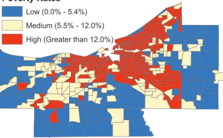
9The negative correlation between vacancy and price is very obvious in maps (figures 2 and 1), but it is not the
theory suggests a specific error structure that differs from the relationship between the prices. In this analysis, we do not have a theoretical reason to use aW2 different fromW1, and using the same spatial weight matrix can introduce collinearity issues. We will refer to the correction involvingW1
as the spatial-lag correction and the correction employing W2 as the spatial-error correction.
In specifying the spatial models, we use a weight matrix based on inverse distances up to one kilometer. Closer sales are given larger weights and further homes are down-weighted. The weights are row-normalized to sum to one, so the product of weight matrices and the price vector or error vector are all in the same units. In the results below, several other spatial corrections are presented and the consistency of the results gives us confidence that our weight matrices are reasonable and effective at removing the spatial autocorrelation bias.
The estimates presented in the results tables apply a spatial-error correction. The spatial-lag estimates, which are very similar, can be found among the robustness checks. Wald tests confirm either model is significantly better than a model without a spatial structure. The test statistics suggest the spatial-error model is a better fit in each of our three main models. In our main results, (table 4), theρ values reflect the extent to which the model’s errors are geographically correlated. The values are between .46 and .68 and are highly significant. This parameter is primarily of interest as a control, with the high, significant value suggesting that it is absorbing unobserved correlation in the error structure and leading to coefficients on the treatment variables that can more plausibly be interpreted as causal. We reportρin the other models, without further discussion, for confirmation of the models’ appropriateness.
If a distressed home decreases the price of a home, that home decreases the prices of homes nearby, and the prices of the homes nearby decrease the price of that home, then the coefficient from the model is understating the impact of an additional distressed home. The average direct treatment impact represents that percentage decrease in home prices if the decline is calculated to impact
the neighboring home prices and then fed back into the original home sale observation (Drukker, Prucha, and Raciborski 2011). The change is calculated and averaged over all observations. When we calculate the average direct treatment impact, we found that it differed from the coefficients by one tenth of a percent or less, and it would be lost in rounding. The results we present may be very slightly understating the impacts.
Two additional concerns are raised in the literature and should be kept in mind when considering this analysis. The causality between foreclosures and falling home prices can run in both directions. When home prices are falling, households in economic distress may not be able to sell their home and downsize or shift to renting. If the recent price downturn has been severe, or if the homeowner put little money down on the home, they may owe more than the home could sell for. Even if they can sell the home, they cannot repay the mortgage unless they have other assets. If a housing market is in the self-reinforcing cycle of falling prices and rising foreclosures, these trends will bias the estimated impact of foreclosed homes. Somewhat parallel arguments could be made that falling house prices increase vacancy and tax delinquency. In our data set, we do not anticipate this being a significant problem because our time period is only fifteen months. Over those fifteen months, the stocks of vacant, delinquent, and foreclosed (within the past twelve months) homes change only modestly with no pronounced trend. Likewise, the time period is not long enough to fully reflect year-over-year price declines. We include indicators for the month of sale in all estimates. These indicators are intended to adjust for the strong seasonality in cold-weather real estate markets, but they could also capture a secular trend. Other studies employing ten years or more of data must take additional steps to account for appreciation or depreciation over that period.
The second estimation issue involves the selection of home sales into our data set. If homes are held off the market by owners hoping for a price recovery, we will not observe their sale prices. If withholding of homes is more frequent near distressed properties, then this could lead to an
underestimate of the impact of the distressed properties on neighboring property values. Lin, Rosenblatt, and Yao specified a model that estimates the selection into a sale and the implied change in the coefficient on the foreclosure count (2009). They find evidence that homes near foreclosures are more likely to be held in the shadow inventory, but the effect on estimates of a foreclosure’s impact is too small to be of great concern.
Most regional economists and policymakers would agree that a data set that covers an entire urbanized county, as ours does, represents several separate housing markets, rather than one. For an average buyer, many high-cost neighborhoods would offer no options within their budget constraint. Likewise, high-income buyers would not consider a home of any type or price if it is in a low-performing school district or high-crime neighborhood. When the models are estimated on a pooled data set, the coefficients are an average across all types of buyers. It is useful to know how the impact of a distressed home differs in high-income verses low-income neighborhoods, so we estimate our models on several submarkets.
The specification of our model is motivated by some practical considerations. First, we are interested in helping policymakers identify types of distressed homes that have the greatest negative impact on neighboring property values. Therefore, we are dividing the homes into counts based on which markers of distress they exhibit, and not allowing them to contribute to multiple counts. While many papers in the literature use multiple buffers to demonstrate the distance decay of the impacts of a disamenity, we primarily report the impacts within one buffer.10 We chose the 500
foot buffer based on findings in previous studies that suggest at 500 feet, the impact of a foreclosure is still significant. A smaller buffer will show a larger impact, but it misses many of the sales that are treated. We are reporting coefficients for five counts in three submarkets, which is challenging to interpret. Multiplying the number of coefficients by additional buffers would make the results
much more difficult to relay to policymakers and is not justified by the additional information in this situation.
To briefly review, we expect each indicator of distress – vacancy, delinquency, and foreclosure – to be associated with lower sales prices for nearby homes after controlling for prevailing neigh-borhood prices and observable characteristics. Vacant homes do not contribute to the vibrancy or security of a neighborhood. In many cases, no one is attending to their appearance daily, so grass is mowed less frequently, snow is not cleared, leaves are not raked, etc. Some of this may be offset if the home is on the market and the sellers have invested in “curb appeal” cosmetic improvements. Unless the home is vacant because it is undergoing major renovations, or awaiting a rental tenant, then the home is either a unit on the market or part of the shadow inventory. The shadow inventory consists of homes owned by individuals or institutions that want to sell, but are not actively marketing because they are hoping the market will improve. When a single lender owns many delinquent loans secured by properties in close proximity to one another, and in markets where there is relatively weak housing demand, the lender may deliberately pace the marketing of foreclosed properties. In either case, these vacant homes (which are often easy to identify in person) signal to buyers that the market is flush with inventory and shadow inventory, and therefore they can bargain for low prices.
The case of delinquency is more subtle. One can reasonably say that it is not visible on the street and very few people look up the tax delinquency status of neighboring homes.11 For homes that
only have tax delinquency, we believe it serves as an objective measure of distress for the property. If the homeowner is unwilling or unable to pay their property taxes, which eventually results in tax-foreclosure, it is very likely that they are unable or unwilling to maintain the property. Poor 11While we a referring to the data as tax delinquency data, it does include some uncollected code violation and
nuisance abatement fines as described in section 3. Since these vary widely between jurisdictions, we attempt to exclude them from the analysis. In many cases, code violations are visible from the street.
maintenance of neighboring properties is visible to home purchasers if any exterior or landscaping work is needed.
The impact of foreclosure is more direct, and therefore, we might expect its per unit impact to be larger. With the exception of strategic defaults, every household that went through a foreclosure has experienced financial distress. When the homeowner accepts that they will likely or certainly lose the home, they no longer have an incentive to invest anything in maintenance. In our data, foreclosures are indicated after the sheriff sale, so the purchasers may have paid off the property’s tax delinquency. If no third party investor bids above the lending institution’s auction reserve, the reserve is recorded as the sale price and the lender takes possession of the property. In many cases, these homes are back on the market or being held as shadow inventory by the lender (Whitaker 2011). If the home is sold out of REO, a second transaction has been recorded at a discounted price. The direct link between these foreclosure-related sales and other sales is the comparables or appraisal process. The foreclosed homes will be considered by sellers, purchasers, and lenders in determining the value of a nearby non-foreclosure property.
We begin with separate counts of each combination of distress because we think homes in different stages of the process will have very different impacts on nearby homes. When past studies have estimated the impact of foreclosures, they are rolling together homes that were just auctioned and are bank owned, homes sold out of REO to speculators that are vacant and delinquent, and homes sold to families that have paid the property taxes and occupied the home. Our parcel-level data with all three measures will reveal if certain combinations of distress indicators matter more than others.
3
Data
The bulk of the data used in our analysis is an administrative dataset maintained to track property transactions, property-tax delinquency, and assessed values for taxation. These data contain a rich set of characteristics for all residences in the county. The records are used in property tax assessments and are updated triennially and with permit data.12 We include measures or indicators of the following as controls: bedrooms, bathrooms, vintage, style (Cape Cod, Colonial, etc.), lot size, condition, construction quality, exterior material, heat and cooling systems, garages, attics, porches, and fireplaces. We supplement the house characteristic data with measures of the poverty rate and the college attainment rate for each census tract using estimates from the 2005-2009 American Community Surveys. The vacancy, delinquency, and foreclosure status of the property itself is included as a control. The vacancy and delinquency measures have large, highly-significant influences on the sale prices, and they improve our model over others that could only control for the foreclosure status.
The county fiscal officer also maintains records of all sales with the key elements of dollar amount, date, seller, and purchaser. Data on tax-delinquency is updated semiannually. We use two tax-delinquency files. The first is a list of parcels that were delinquent anytime in 2010, and the second is a list of properties that were delinquent at any time between January and June 2011. The delinquent amount appears in the record along with any payments that have been made toward it, even complete repayments. The dates when the properties enter or exit delinquency are not available, so these data are static within one year or the other. We identified in the dataset the properties that have missed a biennial payment by flagging only observations in which the delinquency amount is at least 40 percent of the annual net tax bill. This eliminates minor 12If a property owner requests a permit to add an addition on their house, for example, the assessor will estimate
accounting errors (there are hundreds of delinquencies of a few dollars or cents) and the minor code violations. Housing codes vary widely across jurisdictions in their stringency, enforcement, and recording with the county. The Cuyahoga County fiscal officer, like many county departments nationwide, makes tax delinquency data available for download.13
One novel dataset that is being used for the first time (to the best of our knowledge) is the USPS vacancy data. This dataset is created when postal carriers observe that a home has been vacant for 90 days and record it as such in the USPS’s main address database (this data does not include short-term or seasonal vacancies). This prevents mail addressed to the vacant home from continuously being sorted into the route’s load and carried back at the end of the day. The address database, including vacancy status, is routinely audited and maintained at an accuracy level above 95 percent. To further increase efficiency, the USPS makes this data commercially available to direct mailers. The companies can run their mailing lists through a software program that marks each record if the address is vacant. Mailings are not prepared for these addresses, so wasted printing and postage is avoided. The USPS provides this data to private contractors who sell subscription services. For our research purposes, we have subscribed to the vacancy data since April 2010. We run our list of Cuyahoga County addresses through the software, and create a panel of vacancy indicators.
For this analysis, we use the fifteen months of sales data that we have been able to link to complete vacancy data. This covers 11,361 sales in Cuyahoga County between April 1, 2010 and June 30, 2011. We have attempted to exclude non-arms-length sales, starting by excluding sales involving personal trusts and spouses. We exclude bulk purchases, where the price paid for a bundle of properties is recorded for each property in the transaction. In these cases, it is not clear what 13Cuyahoga County makes its data available via Northeast Ohio Community and Neighborhood Data for Organizing
portion of the total prices should be related to the individual properties. We exclude sheriff sales in which a bank or federal agency repurchases a home on which it holds the mortgage. These prices reflect the lender’s auction reserve rather than the market value of the home. The sales data are limited to single family homes. Multifamily buildings are counted in the vacancy, delinquency, and foreclosure counts. Buildings add zero or one to the counts, regardless of how many units they have. A multi-family building is considered vacant if less than 25 percent of its units are occupied. Apartments generally pay taxes via one parcel number while condo parcels must be grouped by building to determine if the building has over 75 percent delinquent units, and thus adds to the delinquency counts of neighboring home sales.
3.1 Descriptive Statistics
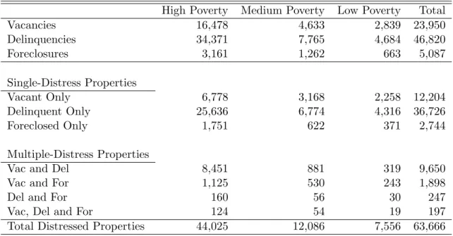
In this section, and in the results, we will present descriptive statistics and models estimated separately in high-, medium-, and low-poverty submarkets. By comparing the results from the submarkets with pooled results, it is evident that pooling hides important differences. Table 1 summarizes the monthly counts of distressed properties.14 Note that delinquencies are the most
common indicator of distress, with vacancy the next most common. The counts of distressed properties in the 500 foot buffers around the home sales are described in Table 2. The (pooled) average home sells with four vacancies, eight delinquencies and one foreclosure within 500 feet. Not surprisingly, all counts are higher in high-poverty census tracts and lower in low-poverty census tracts. To place the counts in context, we need to think about the distribution of neighboring parcels. A home in a low-density exurb may only have a handful of neighbors within 500 feet that could impact its value. In contrast, a home in the densest tract can have over 200 neighbors. The mean number of parcels in a home’s 500 foot buffer is 98 and the standard deviation is 45.
14More extensive descriptive statistics with standard deviations, maximums, minimums, cross tabulations, and
Maps of one month’s vacancies and median sales prices (figures 1 and 2) illustrate that the distribution of vacancies is different in low-price versus high-price areas. Maps of delinquencies and foreclosures have similar patterns. The counts of the different types of distressed homes are positively correlated with one another. Most of the observations of the counts are in the low single digits, and zeros are common. However, there are homes in distressed neighborhoods that are treated by very high counts of all types of distressed properties.
4
Results
Table 3 presents the results of the three submarket models, and a pooled model, each with seven separate distress counts.15 The coefficients on the property characteristics and month indicators
(not shown) are significant in most cases and have the expected signs.16 Counts of vacant (only) and delinquent (only) homes have negative impacts between 1.1 and 2.1 percent in each submarket, with five of the six estimates being statistically significant.
Homes that have been abandoned without going through a recent foreclosure should be counted in the vacant-delinquent category. It seems logical that vacant-delinquent homes would have at least as large an impact as a home with only one of the markers of distress. This hypothesis is supported in the medium-poverty market, but does not hold in the other two. Vacant-delinquent homes are quite common in high-poverty neighborhoods, as indicated by an average count of 4.29 VD homes near a sale in a high-poverty neighborhood (see Table 2). However, the counts of delinquent homes are even higher, and there is a correlation of .75 between the two counts. While a significant negative impact of 1 percent per additional unit is ascribed to vacant-delinquent homes in high-15To calculate the estimates reported here, we use a recently released routine from StataCorp. The package, called
sppack, creates spatial weight matrices and estimates spatial models using a maximum likelihood routine (Drukker, Peng, Prucha, and Raciborski 2011, Drukker, Prucha, and Raciborski 2011).
poverty tracts, the counts of delinquent homes explain more of the variation. In low-poverty areas, vacant-delinquent homes and tax-current foreclosures are present in similar numbers. In these areas, vacant-delinquent homes are certainly distressed, but probably not completely abandoned. The contrast between the large negative impact of the recent foreclosures and the smaller, insignificant result for vacant-delinquent homes may reflect the influence of foreclosures through the recording of discounted sales. Of the four measures involving foreclosure, vacant-foreclosures (tax-current) have the most significant coefficients. Some of the foreclosure coefficients are positive, which is not in keeping with the literature, and begs further exploration.
When all seven distress counts are included for three submarkets, this requires presenting twenty-one coefficients of interest. Results this complex are challenging to interpret and extremely difficult to convey to a general audience, so we considered more parsimonious models that could maintain the important disaggregations.17 Also, if one takes a treatment with a significant impact,
such as foreclosures, and divides its counts by a less important categorization, such as vacancy, there is a possibility of attenuating the coefficients by introducing multicollinearity and measure-ment error. Throughout the remainder of the presentation of the results, most of the models are estimated with the distressed property counts placed in five categories.18 Within the foreclosed home counts, we combined the counts divided by vacancy, but maintained the distinction based on tax-delinquency. The tax status of foreclosed homes proves to be a very informative distinction in high-poverty neighborhoods. In each case where the counts are combined, the resulting coefficient is 17We estimated a seven-treatment equivalent of every model for which it is possible. These estimates are available
from the authors upon request.
18We formally tested if the coefficients for vacant and occupied (tax-current) foreclosures were significantly different
from one another. Likewise, we tested if the vacant and occupied delinquent-foreclosure coefficients were different. In both tests within all three submarkets, the coefficients were not significantly different from one another. If the coefficients were significantly different from one another, combining the counts would less appealing.
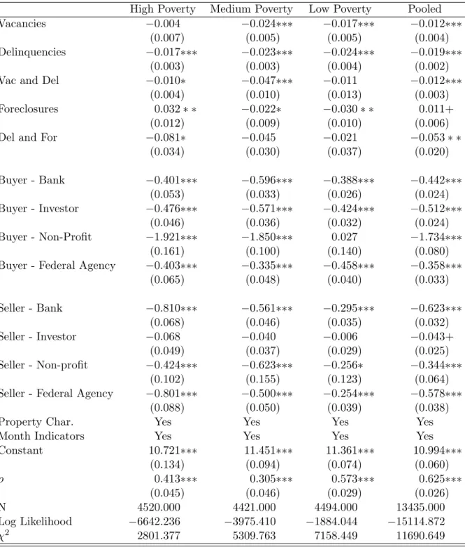
a combination of the two impacts, weighted by the frequency of the distressed property treatments. Our main results appear in table 4. The model suggests that an additional vacant property within 500 feet reduces the sales price of a home by 1.7 percent in low-poverty neighborhoods and 2.1 percent in medium-poverty neighborhoods. Tax delinquent properties have very similar impacts on a per-unit basis (1.8 and 1.9 percent respectively) , but these coefficients would be multiplied by higher counts because delinquent properties are roughly twice as numerous than vacancies. In medium- and low-poverty neighborhoods, having a recent foreclosure near a sale has a large negative impact on the sale price, as expected. A recent foreclosure within 500 feet decreases the sale price by 2.7 percent in medium-poverty tracts and 4.6 percent in low-poverty tracts. Delinquent-foreclosure counts in medium- and low-poverty neighborhoods have small to modest positive coefficients, but much larger standard errors.
Foreclosed homes in high-poverty census tracts display a completely different phenomenon. In poor neighborhoods, recent foreclosures display a marginally significant, positive relationship with nearby sales prices. While it is not plausible that buyers actually value buying near a recent foreclosure, this positive correlation is consistent with selective foreclosure by mortgage holders. In these census tracts, where home values are often lower than transaction and maintenance costs (under $10,000), only homes that are in relatively good condition and on relatively desirable blocks will resell for a value high enough to justify the cost of foreclosure. In this way, a recent foreclosure is associated with higher home values among near-neighbor homes. In contrast, the impact of a tax-delinquent recent foreclosure is -7.6 percent in high-poverty neighborhoods. After the sheriff sale, if either the mortgage holder or the investor that purchased the property has decided not to pay the property taxes, it is very likely that they have abandoned the property. This result suggests that municipalities could identify the most damaging distressed properties in poor areas with two pieces of data they already have in hand, namely recent sheriff sales and the tax status of those
parcels.
The contrast between the submarket results and the pooled results demonstrates the need for different approaches in different areas. Disregarding market differences with pooled results leads to the erroneous conclusion that tax-current foreclosures have no impact at all! It is also evident that tax-delinquent foreclosures in high-poverty areas are driving the negative impact that appears in the pooled results. Focusing only on tax-delinquent foreclosures in medium- and low-poverty areas would not be an effective strategy.
4.1 Comparison to Previous Studies
In the submarket estimates, we report three large, significant negative impacts from recently fore-closed homes. These range from 2.7 percent for a tax-current foreclosure in a medium-poverty tract to 7.6 percent for a tax-delinquent foreclosure in a high-poverty tract. Our findings are in the higher end of the range of negative impacts from a neighboring foreclosed home that were found in the previous studies discussed in section 1.1. The large coefficients on the foreclosure counts may reflect a weak housing market, deep into the housing bust. In 2010 and 2011, Cuyahoga County had a very high inventory of homes for sale. Prices had been declining for several years and showed minimal indications of recovering. Home prices are usually sticky because sellers need to repay their mortgages, and they anchor their perception of their home’s value based on the price they paid. However, by 2010, many owners were capitulating and accepting lower prices. Most of the previous foreclosure impact studies were looking for lowering of values in markets with various upward pressures.
One of the contributions we promised was to correct the estimate of the impact of foreclosures by taking into account other distressed properties in the neighborhood and properties with multiple indicators of distress. In table 5, we present the results of models estimated with each of the counts
alone (models I-III) and foreclosures divided by tax-status alone (model IV). Contrasting these models with the main model (V), or a non-exclusive count model (VI) demonstrates that the impact of foreclosure may be overstated in the absence of vacancy and delinquency measures.19 Even after
dividing the sample into submarkets and controlling for spatial correlation, part of the estimated foreclosure impact is via its serving as a proxy for nearby vacant and delinquent properties. The contrast between model III and model VI gives the best illustration of how the results of previous studies might change if they incorporated vacancy and delinquency data. In areas with relatively strong housing demand, the estimate of the impact of a recent foreclosure declines by 31 percent in the presence of other distress measures.
It is common in the literature to report the results in several different distance buffers to demonstrate the rate of distance decay in the impact of the distressed property. Table 6 shows the results of estimating the model with two exclusive counts in a small (<250ft) and large (250-1000ft) buffer. Our results are consistent with previous research. The negative impacts of distressed properties are generally larger when the properties are closer to the sale. There is an alternate interpretation of these results like these that is made by researchers who emphasize the endogeniety of foreclosure. If falling home prices cause foreclosures and foreclosures lower home prices, then spatial controls may not be sufficient. The later data will feature higher foreclosure counts and lower prices relative to the earlier data, and the coefficient on foreclosure will be overstated because it reflects both impacts. Similar processes could be at work with vacancy and tax delinquency. Some studies include foreclosure counts in an outer ring around the sold home to control for the prevailing frequency of foreclosure in the area. The coefficients on the inner-buffer counts are presented as having reduced bias from the endogeneity of foreclosures. In this interpretation of table 6, there 19By “non-exclusive” we mean the distress counts are made separately. A home with multiple markers of distress
contributes to more than one count. For example, a delinquent-foreclosed house is counted along with all other foreclosures, and the same house also adds one to the delinquency count.
are significant negative impacts from neighboring vacant homes in medium- and low-poverty areas, at -3.5 and -2.5 percent respectively. Delinquent homes have significant negative impacts in high-and low-poverty tracts. The coefficients on tax-current foreclosures are of consequential magnitude, but neither approaches significance. The other coefficients are a mixture of insignificant results. If we hold to this spatial interpretation of the results, we would have to conclude that vacancy and delinquency have large impacts on property values, but foreclosure has no measurable impact.
4.2 Non-Arm’s Length Sales
As discussed in section 3, we excluded sales in which the lender was reclaiming a property used as collateral for a mortgage. Before this exclusion, at least 15 percent of the sales in our data involved an institutional buyer, seller, or both. If we return those sales to the dataset, and estimate the models with an indicator for an institutional buyer or seller, we see that the treatment coefficients (table 7) are similar to those of the main model. Controlling for characteristics of the homes, the discounts recorded for homes entering and exiting REO status are enormous. When a bank or federal agency reclaims a home at a sheriff sale, they set auction reserves between 34 and 56 percent (depending on the neighborhood) less than the sale price for an equivalent property in an ordinary sale. The discount for homes coming out of REO is even steeper in high-poverty areas, at 81 percent. The repossessors appear to be recovering some value in the low-poverty areas, but taking losses in high-poverty areas. Investors, in sharp contrast, buy at a 40 to 55 percent discount and sell near the average market price. For non-profit ”buyers,” the estimates return nonsensical coefficients below -1. This is because non-profit are given homes more often than they actually purchase them, and prices far outside the rest of the price distribution are recorded (such as $10 or $100).
4.3 Other submarket definitions
In table 8, we present model estimates with the observations grouped by different definitions of submarkets. The first grouping is by central city, inner-ring and outer-ring suburbs. From this arrangement, we learn that the inner-ring suburbs have the strongest price penalty for a home being near a delinquent-foreclosed property. The positive correlation between foreclosure sales prices is larger in the central city model than in the high-poverty model, and it is significant at the five percent level. Tax-delinquent homes have large negative impacts in all areas (1.1 to 2.1 percent).
The next two sets of models sort census tracts by vacancy rates and the pre-existing (2006-2009) median home prices. The cut-points are selected to place approximately a third of the sales into each category. Vacancy is positively correlated with poverty, and home prices are negatively correlated with poverty. However, the correlations are not exact, so each change in the submarket definition shifts dozens of census tracts up and down. It is worth noting that submarkets defined by vacancy levels feature reduced variation of this independent variable of interest, just as defining sub-markets by price will narrow the distributions of the dependent variable.
The basic pattern of the main results is visible in both alternate market definitions. With census tracts grouped by vacancy rate, several of the coefficients are smaller than their equivalent with the poverty-level grouping. The estimated impact of vacancies, delinquencies, and foreclosures are all lower in neighborhoods defined by low vacancy compared to a sub-sample defined by low poverty. Vacant-delinquent homes have a larger negative impact if the sample is defined by medium-vacancy rather than medium-poverty.
When pre-existing home prices are used to group the census tracts, the most of the coefficients are larger in magnitude than their equivalent in the main models. The positive coefficient on foreclosures is large and significant in low-price areas, and the negative coefficients on foreclosures
in medium- and high-price areas are also larger than their comparable figures from the poverty submarket (main) results. The coefficient on vacancies in medium-priced areas is surprisingly small, and the coefficient on delinquent-foreclosed homes in low-priced areas is not significant.
4.4 Robustness Checks
As discussed in section 2, there are several options for addressing the spatial correlation between home prices. We attempted five alternate spatial corrections and two corrections for the skewness of the distressed property counts. For the sake of brevity, we have summarized the coefficients in figure 4, rather than seven additional tables.20 In the graph, a letter corresponding to the model
is placed along a line corresponding to one of the five treatments within the three submarkets. If the coefficient is significant at the five percent level, it is placed above the line. If it is marginally significant (.05 <p<.1), it is placed on the line, and if it is not significant, it is placed below.
Model B is an OLS estimate with no spatial correction to the coefficients. As we would expect, the coefficients are larger than the spatially corrected models in 11 of the 15 cases because they are letting the distress counts reflect the variation of other distressed properties. In section 2, we discussed the spatial lag model and the results of that estimate are represented by C. The differences between the spatial-lag (C) and the spatial-error models (A) are minor with the exception of the negative impact of vacant-delinquent homes in medium-poverty areas. The spatial lag model gives an estimate of -4.4 percent, 1.7 points above the spatial-error model estimate.
Model D uses census tract fixed effects to capture unobserved local amenities and disamenities. In high-poverty areas, the estimate with census tract indicators (D) suggests a larger role for vacant homes, while decreasing the estimated impact of delinquent and vacant-delinquent homes relative to their main (A) model coefficients. Forcing the model to use only the variation within census tracts
is quite limiting. Approximately one quarter of the high-poverty census tracts have five or fewer sales observed. The poor neighborhoods are also usually denser, which means distressed properties treat more sales within the geographically smaller tracts. Of the seven significant coefficients in the medium- and low-poverty models, only one (vacant-delinquent in medium-poverty) becomes insignificant with tract fixed effects. The coefficients on delinquencies in medium-poverty markets and foreclosures in low-poverty markets are reduced, but remain at least marginally significant.
The data can locate each sold home in a jurisdiction, and it is reasonable to think the jurisdiction has important effects on the home price. Thus, an indicator of the jurisdiction should capture a lot of important unobserved spatial heterogeneity. In Cuyahoga County, cities correspond to significant differences in property taxes and provide very different levels of city services. They are usually grouped with one or two similar cities into school districts. Property taxes and school districts are known to have large impacts on home values (Oates 1969, Downes and Zabel 2002). When city indicators are included in the model without a spatial error correction (E), most of the results persist in magnitude and significance. Adding a city-specific time trend (F) changes the results only slightly.
The counts of vacancies, delinquencies, vacant-delinquencies, and tax-current foreclosures are skewed. Most of the counts are below five, with a handful of homes being sold near 20 or even 50 distressed properties. Model G includes an indicator for observations that are above the 95th percentile for any of these four counts. The indicator is interacted with the counts to allow for a different slope at high levels. Model H excludes the observations with the high counts.21 In models
G and H, the significant estimated impacts of vacancy, delinquency and foreclosure all maintain at least marginal significance. These results suggest it is safe to say that a few unusually high 21These estimates also exclude observations with delinquent-foreclosures above 2. DF counts above 2 are only found
in high-poverty areas, so we do not try to address them in model H. Doing so would require including additional indicator and interaction terms in one submarket, but not the other two.
observations are not driving the findings. In the cases of vacant-delinquencies, foreclosures, and delinquent foreclosures in high-poverty areas, and foreclosures in low-poverty areas, the coefficients are larger when the highest counts are interacted or removed. This suggests the marginal impact of the first few distressed properties in these counts are underestimated when a linear fits combines their effect with the lower marginal impact of additional units in a high count.
The groupings of significant coefficients suggest that the estimated impact of vacancy and delinquency in medium- and low-poverty submarkets are very robust. In high-poverty tracts, the estimated impacts of vacancy are tightly grouped, but not significant. The high-poverty coefficients on delinquency are all similar except when census-tract fixed effects are included (D). On the foreclosure measures, all of the models agree that there is a positive correlation between tax-current foreclosures and sale prices in high-poverty neighborhoods. This result is at least marginally significant in the presence of any spatial correction. In low-poverty areas, the estimates of the negative impact of foreclosures are sensitive to the corrections for spatial correlation, but they are always negative and significant. In medium-poverty areas, the estimates of foreclosure are tightly grouped and at least marginally significant in all but one model.
5
Policy Implications
5.1 Removing Blight
Using our main model, we attempted a simple experiment to estimate the potential benefit from eliminating some of the distressed properties. We returned to our model and re-predicted the sale prices four times, each time setting the counts on one of the distressed property types to zero. We sum the increase in the predicted values and divide it by the average number of units with the marker of distress in a month. This gives a predicted per-unit increase in transaction values. The
values are implicitly weighted by the sales activity the distressed properties actually influenced, but they suggest a proportional increase in property values of unsold homes as well. This benefit could be weighed against the cost of a program that alleviates distress on properties.
Table 9 presents the results of the experiment. To place the table in context, the total value of all home transactions in the dataset is $1.4 billion. In per-unit terms, foreclosures lead to the largest losses of value at $4,665 for tax-current foreclosures in medium-poverty neighborhoods to $9,489 per tax-current foreclosure in low-poverty neighborhoods. The total values, before dividing by the units, tell a different story. The total value lost to sellers due to homes that are vacant, delinquent, or both is estimated at $90 million versus $12.7 million lost due to foreclosures.
If our model is correct, attempting to eliminate the approximately 3,000 foreclosures that affect the high-poverty tracts would be as fruitless as it would be overwhelming. Putting a laser focus on the approximately 300 homes that are foreclosed and delinquent in high-poverty neighborhoods is more feasible. Recovering $1.5 million of value for sellers might not justify the expense of a program, but when the increased value of nearby homes is taken into consideration, the benefits would be much larger. A successful program would have the indirect effect of stabilizing the property tax base. In medium- and low-poverty areas, preventing foreclosures could salvage some of the $11 million lost to sellers near foreclosed homes.
In this experiment, we are assuming a targeting by type of distress and type of neighborhood. Targeting would have to take into account equity concerns because preventing a foreclosure in a neighborhood where homes sell for $300,000 may have a larger percentage and dollar benefit than preventing a foreclosure in a neighborhood with $50,000 homes, but such assistance is rarely targeted to high-income neighborhoods.
While it is simple in a dataset to remove vacancy or delinquency observations, designing a program to successfully eliminate these conditions in actual homes is very challenging. In the case
of delinquency, policymakers should bear in mind that it is unlikely that property tax delinquency itself that lowers property values, but rather the neglect associated with property tax-delinquency. Forgiving delinquent property taxes does not change the fact that the homeowner is unable or unwilling to invest in his or her property. Likewise, eliminating vacancies in homes that are not candidates for demolition would require attracting migration to the region or stimulating household formation.
Finally, if lenders are strategically foreclosing on the few desirable properties in highly distressed areas, there is no easy way for policymakers to obtain the properties that are mortgaged and in default. In these cases, lenders maintain their first-position security interests, which encumber properties and prevent redevelopment. In such cases, creative ways to encourage foreclosure or the surrender of the lenders’ leans would need to be pursued before the property could be eliminated.
5.2 Housing Market Interventions
Since the foreclosure crisis began, state and federal governments have spent billions of dollars on various foreclosure prevention programs, in part to combat the negative externalities prior research has associated with foreclosure. Our research suggests that vacancy and abandonment in less robust housing markets should be receiving at least as much attention as foreclosures. Indeed, this has long been recognized by community development practitioners, who are often more concerned with the vacancy and abandonment that sometimes results from foreclosure than the foreclosures themselves.
Foreclosures are currently a serious problem across the United States, but they are not long-term problems like vacancy and abandonment. As the economy improves and borrowers are better able to service their debt, the number of foreclosures will drop. In the meantime, some foreclosures are quickly reoccupied by owners or purchased by an attentive landlord who rents the property out.
Thus, not every prevented foreclosure will mitigate the externalities associated with vacancy and abandonment. But as long as policy remains focused on the construction of new housing over the maintenance of older ones, vacancy and abandonment will persist. To date, there have not been many policy responses aimed specifically at vacancy and abandonment, and most are untested.
For example, vacancy registration ordinances have arisen in municipalities across the United States. They usually require a property to be registered within a specific number of days of becoming vacant, and subject the property to additional housing code inspections while registered or at the point of sale. While they do not remediate distressed property, they may incentivize property owners to reoccupy vacant property to avoid registration, or to take better care of the property in light of the additional inspections. To date, there has been no research done on the effectiveness of these programs.
When combating vacancy and abandonment, modern land banking is one strategy that shows promise. Modern land banks are public or quasi-public entities charged with acquiring, remediat-ing, and placing vacant and abandoned homes back into productive use (Fitzpatrick 2010). The most intriguing modern land banks are organized under Ohio law, with statutorily defined pub-lic missions, stable funding mechanisms, and significantly more power and flexibility than other modern and historic land banks. In less-robust markets like Genesee County, MI and Cuyahoga County, OH, land banks often focus upon the demolition and repurposing of older, distressed hous-ing stock. Like studies of vacancy ordinances, evaluations of modern land banks have been very limited (Griswold and Norris 2007).
Finally, our results illustrate the difficult decisions that must be made when deciding how to allocate resources to combat vacancy and abandonment. It appears that the benefits of each marginal dollar spent on mitigating vacancy and abandonment would be higher in medium- and low-poverty areas. However, the incidence of vacancy and abandonment is highest in high-poverty