Two Dimensional Image Denoising Using Partial Differential Equations with a Constraint on High Dimensional Domains
Carl Lederman1
1
Department of Mathematics, University of California, Los Angeles
Abstract
In the proposed method for image denoising, an operator is defined to take the image data to a high dimensional (e.g. ten dimensions) image representation in a patch attribute space. A partial differential equation is run in this space with the constraint that that the high dimensional representation conforms to a true two dimensional image. The high dimensional PDE is modeled using a simplified meshfree method and the constraint enforced with a projection that naturally follows from the defined operator. This leads to an updating of pixel values, not by an averaging procedure, but through a search for an optimal solution to a system of overdetermined equations. This approach is explored using the reverse heat equation, which deblurs when run on the image domain, but when run on the high dimensional patch attribute space formulated here, it denoises.
1 Introduction
1.1 Non-local Means and Semi-local Means
The basic approach of the non-local means denoising method [5] is to identify pixels anywhere in the noisy image that should have a similar value in the true image (that is, the image without noise) and then average these pixels together to reduce the noise. Determining which pixels should be averaged together is typically done by comparing the difference between patches of pixels around the pixel of interest (often a 5 by 5 pixel patch is used). Many modifications and improvements have been made in subsequent works including [3], [7], [8], [11], [13], [15], [17], [18], [19] and [20], some of which are discussed in more detail below. The non-local means approach contrasts to earlier methods that can be interpreted as local averaging methods. Local averaging can be implemented in careful ways to avoid the worst effects of local averaging. For example, the well known method [16] can be interpreted as a local averaging method that is careful to avoid averaging across sharp edges in the images. But this method will still remove more intricate patterns and textures.
Semi-local means is a slight variant on the non-local means method. It differs only in that patches can only be compared if they are nearby, typically meaning that they fall within the same small square search window. The semi-local means method has a computational complexity of where is the number of pixels and is the window size. This works well and quickly if patterns in the image repeat nearby in the image. This may not always be the case and, furthermore, in some applications the objects of the greatest interest may not repeat frequently, such unusual growths in a set of medical images or an aerial photo with small ships in an ocean. Yet, increasing the window size does not necessarily lead to a better overall result, as shown in [8] for example. Twenty-five noisy pixels is not sufficient to describe any object and so it is possible that patches that are similar with noise may really not be, and thus in this case an averaging procedure will not effectively lead to a closer approximation to the true image. A small window size makes these bad patch comparisons less likely. Furthermore, a large makes the computation impractical, though this has been addressed using filtering methods (discussed below).
In the proposed method, the pixel values are not updated with an averaging procedure. Instead an overdetermined systems of equations is constructed and the pixel values are updated by finding an optimal solution to this system. The practical consequences of this is that the denoising is much less affected by incorrect patch comparisons and a lack of good patch comparisons. A pixel value can update correctly even if its surrounding patch does not resemble any other and a pixel is less susceptible to being
adjusted toward an incorrect value. This results in more noise being removed from the image and less of the true image ending up in the noise removed, as is discussed in the results section.
1.2 Filtering methods
Some nonlocal methods employ so called filtering methods ([4], [11], and [13]) which measure a few patch attributes in advance of the denoising to limit the search range of similar patches when the actual denoising is performed. Usually the number of patch attributes considered is smaller than 25 (4 in [11] and 6 in [13]). Thus the search range could include candidates that are not relevant (just as when 25 patch attributes are considered) but, in addition, could miss some patches that are relevant. Furthermore, in some cases the search range could include the majority of the image, such as when most of the image is a solid single color. These filtering methods are a different sort of approach than what is proposed here and not necessarily incompatible.
1.3 Reverse Heat Equation and Projections
Modified versions of the heat equation have been used in image processing applications for decades [10]. If is simply defined on the image domain, the forward heat equation, , will remove noise but blur out the image. The reverse heat equation will deblur but increase the noise in the process. In [6] the reverse heat equation and nonlocal means are conisidered. But the reverse heat equation term is local and used for deblurring and the denoising term is non-local. In [8], a nonlocal positive Laplacian (forward heat equation) is defined for denoising. The nonlocal Laplacian is modified from a graph theory version and the sign is switched so that this nonlocal Laplacian corresponds to the local Laplacian in a special case. New operators can be defined in any way that is appropriate. But here, a new Laplacian is not defined, but merely the classical one used in a different space and this unambiguously results in the reverse heat equation.
Some papers have examined performing operations on the patch attribute space including running partial differential equations, [14],[17], and [18]. In [17] and [18] (two versions from the same authors), a heat equation is run on the patch attribute space and projected onto the image domain. However, their formulation leads to an averaging procedure defined on the image domain which is quite similar to the original non-local means method, as the authors point out. In the proposed method, the formulation naturally leads to the pixels being updated, not by averaging, but through obtaining the solution to an overdetermined system of equations. This is the primary reason why the results presented here are different and improved over the original non-local means method. Another key difference is that the heat equation in [17] is solved using established information about the particular solution of the heat equation, specifically that it can be solved using convolutions with a Gaussian kernel. The proposed method employs a general approach to solving PDEs, meshfree methods, and could therefore be modified to work with other PDEs.
Also of note is that projection methods have been incorporated into numerical schemes for solving fluid dynamics problems [2].
1.4 Meshfree methods
Meshfree methods are a means by which partial differential equations can be numerically implemented [9]. Two main advantages of these methods is that they can work in high dimensional spaces and that they are less restricted by a preset domain on which the PDEs are run. Meshfree methods are chosen here because finite difference and finite element methods are impractical in high dimensional spaces. Two main drawbacks of meshfree methods are the difficulty associated with creating an approximation to an arbitrary function and imposing boundaries constraints. Both of the issues are trivial
in the simplest finite difference and finite element situations. But as is explained in the methods section, neither of these significant difficulties come into play for the proposed denoising approach.
Meshfree methods are not common in image processing applications but include [1] and [12]. Both of these papers use meshfree methods on the image domain, which is not what is done here.
2 Proposed Image Denoising Method
2.1 Construction of high dimensional image representation
The image data is taken to be a vector, , of length , where is the number of grayscale pixels. Each entry of , denoted , gives the single grayscale value of pixel . The proposed method involves creating a linear operator to convert each into a point in 10 dimension space, which is denoted . From these and an estimate about the amount of noise in the image, a high dimensional function
is generated. Locations close to each other in the 2D image may be completely different things and so a local interaction may not be useful for reducing the noise. But the linear operator which takes points from to is such that locations close to each other in this 10 dimensional space are similar things, and so local interactions in this space may be useful for denoising.
Each point is associated with one pixel and the coordinates of the point are determined by computing patch attributes. 10 attributes were heuristically picked as shown in Figure 1. The attributes are the sum of various pixels, shown in gray, multiplied by a normalizing constant so that they have equal significance in the denoising. During the projection step discussed below, pixels will be found that correspond to given attributes. Of note is that 10 attributes specified for one patch give some guidance for how the 25 pixels in the patch will be updated but still allow some flexibility.
Figure 1 The point is at the center of the 5 by 5 patch. The gray pixels are added and normalized to obtain each of the 10 coordinates of .
This procedure can be expressed concisely using the matrix , which has rows by columns, the vector of length , which contains the values of the pixels in the image, and the vector which is of length .
The distance between a point and is measured using the ordinary Euclidean distance.
The basis functions centered at each are related to how far away a is likely to be from its true location without any noise in the image. This will allow points to interact if it is likely that their distance apart is related only to the noise present. The single value is related to the standard deviation of the distance of each from its true location, and is calculated based on an initial estimate of the noise in the image. As the points move during the simulation, it is assumed that they move to reduce the noise. If is equal to at the beginning of the simulation then a crude estimate of the current amount of noise is given by:
A Gaussian function is formed around each . This function appears in various non-local means methods and is also used for basis functions in meshfree methods. It can also be interpreted as a probability distribution function of where is likely to be if no noise were present, though it does not strictly integrate to 1 for numerical implementation reasons when is small.
The function is achieved by simply summing these generating functions g.
Once the function is generated at each time step, it only changes as a result of the points being moved, as described in the next section.
2.2 Updating the High Dimensional Image Representation and Projecting It
The points should change from a more disperse or disordered state to a more ordered one. This result can be achieved by running the reverse heat equation on the high dimensional represenation of
, denoted by .
To compute the Laplacian of at each time step, a local approximation of the function is required at each . This is done by pseudo-randomly selecting 10 nearby points. Selecting any 10 points at random would produce some points that are so far away that their basis functions have a negligible contribution. Selecting the 10 exact nearest neighbors might cause similar points to be selected
at each time step and points that are close enough to have their associated basis functions significantly affect will never be considered. This pseudorandom nearest neighbor search is the slowest step and can be done with computational complexity as good as . Additionally, the reverse heat equation is unstable, and working with very large values of , which would occur if a large number of nearby neighbors are considered, can cause instability.
The function is updated at each time step by moving the points . This is done in order to keep all the relevant information about required to perform the projection encapsulated within the . The number denotes the current time step and the next time step.
The points were creating from an image. However, as soon as these points are moved to obtain there is no longer a correspondence to a true image. The altogether contain values and somehow the best image with values corresponding to this needs to be found. This is done using the aforementioned relation between the image and high dimensional data involving .
The matrices and are sparse and only need to be found once. There are many methods to quickly find the solution to a sparse symmetric positive definite linear system.
2.3 Partial Differential Equation
The partial differential equation involves a high dimensional representation of , denoted by , and a projection which is used to convert the high dimensional representation back to an image. The procedure for creating is described in detail in section 2.1. The projection, , gives the vector of length that best approximates the high dimensional data, denoted . The specific formulation for relates to the linear operator that was used to generate the high dimensional function and is described in detail in section 2.2. A standard fidelity term to the original image is a also present. The vector of length is simply the grayscale pixels values of the original noisy image.
2.4 Summary of Numerical Implementation
The updating of at each time step, where denotes the current time and then next time step, is summarized as follows:
1. Use the points to generate points and the function as described in section 2.1.
2. Update by moving the points to as described in section 2.2. 3. Obtain the that best corresponds to as described in section 2.2 4. Compute using the formula below:
3 Results
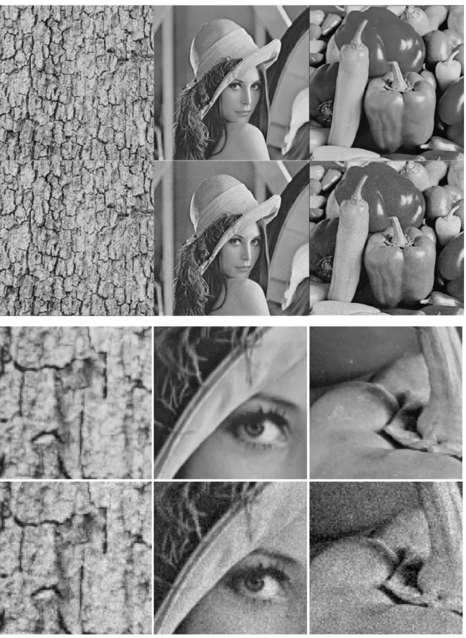
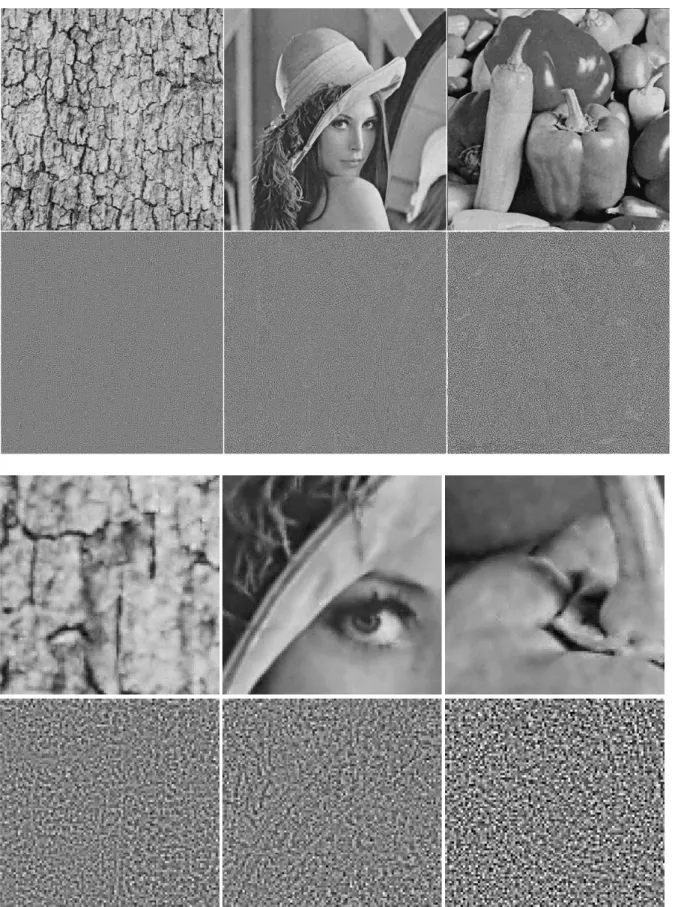
Artificial noise with standard deviation 10 was added to images of bark and Lena, and noise of standard deviation 15 was added to the peppers image as shown in Figure 2. For all noised and denoised images, the signal to noise ratio is computed:
The bar stands for the average of that value over the whole image and the subscript stands for the true image with no noise. As another measure of the denoising quality, the sup norm, or worst error in the image, was computed:
While very simple, this measure is completely unforgiving. If the denoising method removes patterns that are present in the clean, original true image or fails to denoise large parts of the image, this measure will be poor. Also, as discussed previously, in some applications things that occur rarely within an image may be of greater interest than large regions of near constant pixel value. This may be a better measure of how well intricate and rare features are denoised.
The proposed method (Figure 6) is compared to the original non-local means method (Figure 5) [5] as well as two semi-local means methods (Figures 3 and 4) [5] using different patch sizes. The non-local method provides the most direct comparison as the proposed method is also fully non-non-local. But, varying the window and patch size can cause various advantages and disadvantages depending on both the image noise and image content. So different window and patch sizes are considered to provide some evidence that the proposed method gives a denoising result that cannot be achieved by a non/semi-local means method with a careful selection of window and patch size. For all examples the programs were given the true standard deviation as a parameter.
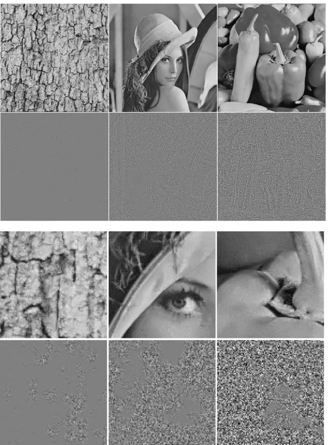
Figure 3 shows the result obtained by the original semi-local means method using a 5 by 5 patch and an 11 by 11 search window. The denoising results for the pepper are quite good as can be seen by the noise removed. Denoising occurs on most of the image and not too much of the true image appears in the noise removed. In the peppers image, most patches are similar to some other nearby patches. In contrast, the denoising result for the bark is extremely poor. For this image, similar patches do not often repeat nearby. Very little of this image is actually denoised. Lena also contains some large regions where very little denoising occurs.
In Figure 4, the window sized remained 11 by 11, but the patch size was reduced to 3 by 3. This resulted in more denoising occurring for the bark image though many areas where no denoising occurred still remain. However, at the same time, Lena's, as well as the peppers, true image shows up more in the noise removed when compared to the 5 by 5 patch.
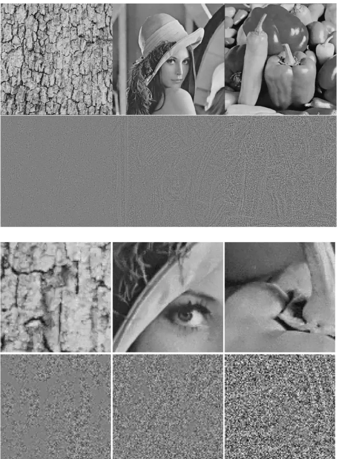
Figure 5 shows the original NL means method with a patch size of 5 by 5 and a search window size of 512 by 512, that is, the entire image. Just as when the patch is reduced in size, increasing the window size results in a trade off where more of the image is denoised yet at the same time more of the true image appears in the noised removed. The SNR is worse in some cases than the semi-local method, but the sup norm is always nearly equivalent or much better than the semi-local methods. So non-local methods may possibly still be a better choice for denoising applications where the object of interest is complicated (that is, difficult to denoise) and does not repeat frequently in the image. Also of note, is that no filtering method was used. If one were employed to break the computationally complexity, the results would likely be worse.
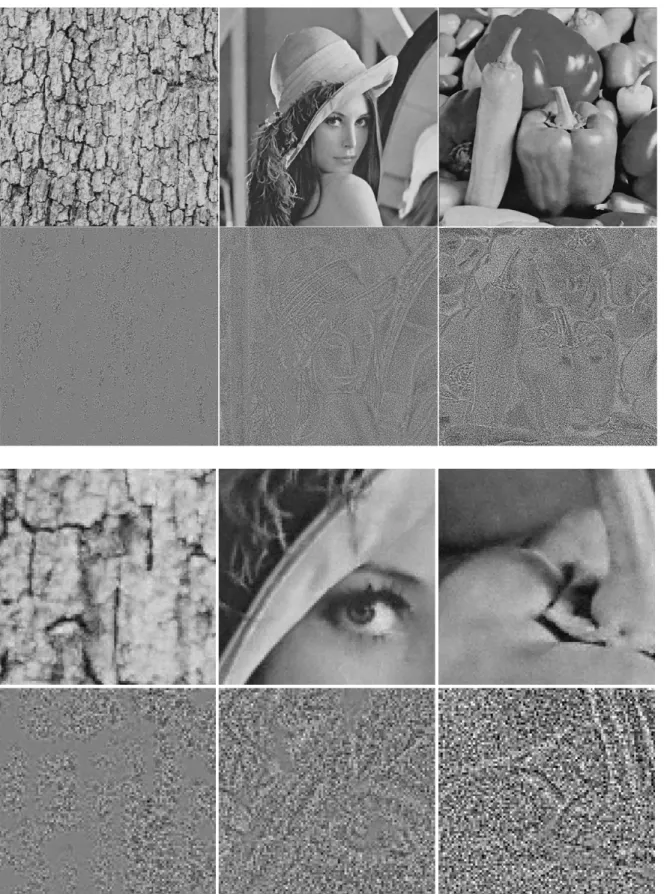
Figures 6 shows the denoising result with proposed method. Unlike any of the previously discussed variations of the original non/semi-local means, significant denoising occurs throughout all three images. At the same time, very little of the true image appears in the noise removed which occurred for the original non/semi-local means only in the large patch and small window situation shown in figure 3 (at the expensive of large image regions not being denoised as discussed). Additionally, both measures of image quality for all three images were either equivalent or superior when compared to all variations of the original non/semi-local means methods. On the negative side, a small amount of blurring seems to be occuring in the proposed method. This could be due to the minimization in the projection step, the Laplacian operator, or a suboptimal choice of patch attributes to measure.
4 Conclusion
The proposed denoising method can effectively compare data throughout an entire image and incorporate it into an effective denoising result. Very little of the true image is removed as noise and significant denoising occurs in every part of the image. The projection step of the proposed method, which involves finding a solution to an overdetermined system, is of great importance to achieving this result.
The computational complexity of the method is not as good the optimal
complexity, but given that even a simple 1D sorting problem has computational complexity, a fully nonlocal method with a complexity would be challenging. Additionally, modified version of the filtering methods may be applicable here to further speed up the method.
Another advantage of this method is that there may be many avenues toward its improvement. The speed and denoising capability of the method depends on several very well studied problems, including selecting local image attributes of interest, partial differential equationss, random nearest neighbor searching, and finding an optimal solution to an overdetermined system.
Acknowledgements
I would like to thank my advisor, Luminita Vese, for the excellent guidance she provided me on this paper.
References
[1] Blasi, G., Francomano, E., Tortorici, A. Toscano, E., "A Smoothed Particle Image Reconstruction method" Calcolo - Special issue devoted to the 2nd Dolomites Workshop on Constructive
Approximation and Applications, 2009 (2010)
[2] Brown, D., Cortez, R., Minion, M., Accurate Projection Methods for the Incompressible Navier-Stokes Equations, Journal of Computational Physics, Volume 168, Issue 2, 10 April 2001, Pages 464-499 [3] Brox, T., Cremers, D. "Iterated Nonlocal Means for Texture Restoration" SSVM 2007, LNCS 4485, pp. 13–24, 2007
[4] Brox, T., Kleinschmidt, O., and Cremers, D., "Efficient Nonlocal Means for Denoising of Textural Patterns" IEEE Transactions on Image Processing, Vol. 17, No. 7, July 2008
[5] Buades, A., Coll, B., Morel, J.M. "A non local algorithm for image denoising" IEEE Computer Vision and Pattern Recognition 2005, Vol 2, pp: 60-65, 2005
[6] Buades, A., Coll, B., and Morel, J.M. "Image enhancement by non-local reverse heat equation" Technical Report 2006-22, Centre de Mathematiques et Leurs Applications, ENS Cachan, 2006.
[7] Coupe, P., Yger, P. , Barillot, C., "Fast Non Local Means Denoising for 3D MR Images" MICCAI 2006, LNCS 4191, pp. 33–40, 2006
[8] Gilboa, G. and Osher S. "Nonlocal Linear Image Regularization and Supervised Segmentation" UCLA CAM Report 06-47 (2006).
[9] Gregory F. Fasshauer "Meshfree Approximation Methods with MATLAB" World Scientific Publishing Co. 2007.
[10] Kovasznay, L. S. G., Joseph, H.M. "Image processing", Proc. IRE, 43 (1955), p. 560
[11] Mahmoudi M., and Sapiro, G., "Fast Image and Video Denoising via Nonlocal Means of Similar Neighborhoods" IEEE Signal Processing Letters, Vol. 12, No. 12, December 2005
[12] Opfer, R. "Multiscale kernels" Advances in Computational Mathematics 25: 357–380 (2006) [13] Orchard, J., Ebrahimi, M., Wong, A.: "Efficient Non-Local-Means Denoising using the SVD" Proceedings of The IEEE International Conference on Image Processing ICIP 2008, San Diego, California, USA, October 12-15 2008
[14] Peyre, G., "Image Processing with Non-Local Spectral Bases" SIAM Journal on Multiscale Modeling and Simulation 7, 2 (2008) 703-730
[15] Pizarro, L. Mrázek, P., Didas, S., Grewenig, S., Weickert J., "Generalised Nonlocal Image Smoothing" Int J Comput Vis (2010) 90: 62–87
[16] Rudin, L., Osher, S., Fatemi, E., "Nonlinear total variation based noise removal algorithms" Physica D, 60:259–268, 1992.
[17] Tschumperle, D., Brun L., "Image Denoising and Registration by PDE’S on the Space of Patches" International Workshop on Local and Non-Local Approximation in Image Processing (2008)
[18] Tschumperle, D., Brun, L., "Non-local image smoothing by applying anisotropic diffusion PDE's in the space of patches" Image Processing (ICIP), 2009 16th IEEE International Conference on pages 2957 - 2960
[19] Wiest-Daessle, N., Prima, S., Coupe, P., Morrissey, S., Barillot, C., "Non-Local Means Variants for Denoising of Diffusion-Weighted and Diffusion Tensor MRI" MICCAI 2007, Part II, LNCS 4792, pp. 344–351, 2007
[20] Zimmer, S., Didas, S., & Weickert, J. (2008). A rotationally invariant block matching strategy improving image denoising with nonlocal means. In Proc. 2008 int. workshop on local and nonlocal approximation in image processing, LNLA 2008, Lausanne, Switzerland, August 2008.
Figure 2 Three images with noise of standard deviation 10 (left), 10 (middle) and 15 (right). Zoomed in portion of image on bottom. SNR is 22.1 (left), 22.9 (middle), and 13.1 (right). Sup norm is 44 (left), 52 (middle), and 77 (right) .
Figure 3 Original SL-means method with an 11 by 11 search window and 5 by 5 patch. Denoised image and removed noise (multiplied by 4) shown. SNR is 24.3 (left), 87.0 (middle), and 79.7 (right). Sup norm is 44 (left), 40 (middle), and 60 (right).
Figure 4 Original SL-means method with an 11 by 11 search window and 3 by 3 patch. Denoised image and removed noise (multiplied by 4) shown. SNR is 30.0 (left), 91.5 (middle), and 76.0 (right). Sup norm is 43 (left), 37 (middle), and 63 (right).
Figure 5 Original NL-means method with whole image search window and 5 by 5 patch. Denoised image and removed noise (multiplied by 4) shown. SNR is 30.9 (left), 91.6 (middle), and 68.8 (right). Sup norm is 40 (left), 38 (middle), and 52 (right).
Figure 6 Proposed method. Denoised image and removed noise (multiplied by 4) shown. SNR is 33.6 (left), 103.8 (middle), and 79.7 (right). Sup norm is 39 (left), 35 (middle), and 50 (right).