T
HE
W
ILLIAM
D
AVIDSON
I
NSTITUTE
AT THE UNIVERSITY OF MICHIGAN BUSINESS SCHOOL
Volatile Interest Rates, Volatile Crime Rates:
A New Argument for Interest Rate Smoothing
By: Garett Jones and Ali M. Kutan
William Davidson Institute Working Paper Number 694
May 2004
Volatile Interest Rates, Volatile Crime Rates: A new argument for interest-rate smoothing
by Garett Jones*† Ali M. Kutan**
*U.S. Senate and Southern Illinois University Edwardsville
** The William Davidson Institute, University of Michigan and Southern Illinois University, Edwardsville
Abstract
Good monetary policy requires estimates of all of its effects: monetary policy impacts traditional economic variables such as output, unemployment rates, and inflation. But does monetary policy influence crime rates? By extending the vector autoregression literature, we derive estimates of the dynamic effect of higher interest rates on crime rates. Higher interest rates have socially and statistically significant positive effects on rates of theft and knife robberies, while effects on rates of burglary and assault are smaller and statistically insignificant. Higher interest rates have no effect on homicide rates. We conclude that monetary policy influences the rate of economically-motivated crimes.
Keywords: crime, monetary policy, vector autoregressive models (VARs). JEL classification: E5 and C3
†Corresponding Author: Department of Economics and Finance, Southern Illinois University, Edwardsville, IL, 62026. garjone@siue.edu. (618) 650-2982. JEL Codes: C22, K42, E52.
I. Introduction
Many observers have investigated the potential factors affecting crime in the U.S. The existing literature has suggested three sets of factors. Earlier studies focus on a benefit and cost analysis of committing crime (Becker, 1968; Ehrlich, 1973, 1981, 1996; and Levitt, 1997). The second set of studies relates crime rates to the state of the economy (Imrohoroğlu, Merlo and Rupert, 2001). Finally, more recent studies argue that labor market conditions (wages and unemployment) can explain changes in crime rate (Freeman, 1996, 1999; Raphael and Winter-Ebmer, 2001; Gould, Weinberg, and Mustard, 2002). Regarding unemployment, the existing empirical evidence has produced mixed results (Freeman, 1996, 1999). The potential effect of wages on crime is generally ignored in the literature. Grogger (1998) and Gould, Weinberg, and Mustard (2002) have recently tackled this issue and found that wage movements, along with other factors such as unemployment, are a significant determinant of crime.
This paper differs from the existing literature in several significant ways. First, this paper is the first to examine whether crime rates in the U.S. are responsive to monetary policy shocks. Second, our study can be interpreted as an extension of the above studies that explain crime rates based on the state of the economy and labor market conditions. Monetary policy shocks, by directly influencing the economic conditions, including the labor market, may affect crime decisions. Therefore, our empirical results have vital policy implications. If monetary policy affects crime significantly, then central banks may choose to include crime as a factor in their objective function when designing an optimal policy. Third, we develop a time-series econometric technique that does not require us to create full-blown structural models of crime, but which can nonetheless estimate the dynamic effect of an exogenous change in interest rates on crime rates.
The rest of the paper is organized as follows. Section 2 explains our empirical methodology followed by data description in Section 3. Empirical findings are reported in Section IV. Final section discusses the policy implications of our results and concludes the paper.
II. Methodology
In this section, we make use of the fact that any vector autoregression (VAR) can be represented as a much simpler vector moving average (VMA) process. Our ultimate objective is to econometrically estimate one set of equations from the VMA process, equations that estimate the impact of monetary policy shocks on crime rates.
We are interested in the time-series properties of an ((m+n) x 1) vector of covariance-stationary variables, yt. We will stack the variables so that the m crime variables are on top, and
the n economic variables are on the bottom:
yt =
ec t cr ty
y
(1) In the Structural Vector Autoregression (SVAR) literature, the current values of ytdepend partially on the lagged values of all of the elements of yt: For example, this month’s
unemployment rate might be related to last month’s unemployment rate and last month’s level of industrial production.
In addition, some elements of this month’s yt will be affected by other elements of this
month’s yt; when the Federal Reserve sets the federal funds rate, for example, their decision will
depend on that month’s consumer price index and that month’s industrial production. This latter situation—where some elements of yt depend on other elements of yt, could conceivably lead to
a classic problem of simultaneous equations, but as we will see, econometric techniques have been developed (summarized by Christiano, Eichenbaum, and Evans (2000)) that provide a tractable solution to this potential problem. Therefore, let us consider the following equation, which jointly characterizes the U.S. economy and the regional economy we are interested in:
yt = α+ Φ0yt +Φ1yt-1+. . .+Φpyt-p+εt (2)
Here, α is an (m+n)x1 vector, the Φ matrices are (m+n)x(m+n), and εt is a vector of
(m+n)x1 shocks to the national and regional economy. These shocks εt are assumed to be
independently and identically distributed, with a diagonal covariance matrix, denoted D. This implies that there are a total of (m+n) shocks hitting the economy each period, but while the diagonal covariance matrix implies that the same-period shocks are uncorrelated with each other, it is possible for each shock to influence more than one element of yt.
For instance, if there is a shock to industrial production this month, that will, of course, immediately influence industrial production; and since this month’s federal funds rate depends in part on this month’s industrial production, the industrial production shock will simultaneously influence this month’s federal funds rate. The combination of same-period relationships between the elements of ytis contained within the matrix Φ0. For now, we will simply note that as long
as Φ0 is invertible, we can make the following transformation:
(I – Φ0)yt = α+Φ1yt-1+. . .+Φpyt-p+εt (3)
yt = (I – Φ0)–1α+(I – Φ0)–1Φ1yt-1+. . .+(I – Φ0)–1Φpyt-p+(I – Φ0)–1εt (4)
and if we define a = (I – Φ0)–1α, and Pi = (I – Φ0)–1Φi, this can be rewritten as
yt = a + P1yt-1+. . .+ Ppyt-p+(I – Φ0)–1εt (5)
Note that in this format, the covariance matrix of et is now ((I – Φ0)–1)D((I – Φ0)–1) , and
hence is unlikely to be a diagonal matrix. This implies that the contemporaneous relationships between the elements of yt are now reflected in the covariance matrix of the disturbance terms.
Our eventual goal is to uncover the underlying disturbances to monetary policy, in order to estimate the effects of these exogenous disturbances on local variables; therefore, we are interested in how the monetary policy disturbance (one of the n nationwide elements of εt)
effects some of the m local elements of yt. This motivates us to rewrite (5) as follows, using L as
the lag operator, where Lpy
t = yt-p:
(I – P1L1– . . .– PpLp)yt = a +(I – Φ0)–1εt (6)
yt = (I – P1L1– . . . – PpLp)–1a +(I – P1L1– . . . – PpLp)–1(I – Φ0)–1εt (7)
The first term on the right hand side of the equation is a constant equal to the mean of the process. This is so because if we take unconditional expectations of both sides,
E(yt) = E((I – P1L1– . . . – PpLp)–1a)+E((I – P1L1– . . . – PpLp)–1(I – Φ0)–1εt) (8)
E(yt) = E((I – P1L1– . . . – PpLp)–1a)+ 0 (9)
Hence, we will simplify notation by referring to (I – P1L1 – . . . – PpLp)–1a) as y.
Hamilton (1992, pps 257-260) demonstrates that any covariance-stationary vector process such as this one can be rewritten as a infinite-lag vector moving-average process. This is the vector extension of the fact that any finite-order autoregressive process has an infinite-order moving average representation. Therefore, we have:
yt = y+(I – Φ0)–1εt + ψ1(I – Φ0)–1εt-1 +ψ2(I – Φ0)–1εt-2 +. . . (10)
If the process is covariance-stationary, then the infinite lags will approach zero matrices. The reader interested in how to construct the ψi matrices is referred to Hamilton’s (1992)
excellent treatment of the issue.
Equation (10) indicates that if we had access to a time series for any one of the disturbance equations, εi
t (e.g., a set of monetary policy disturbances), and also had time series
for one of the elements of ycr
t, (e.g., the U.S. burglary rate), then we could regress the burglary
rate on the monetary policy disturbances and a constant, and the result would be unbiased, asymptotically valid estimates of individual element of the (m+n)x(m+n) matrices ψi(I – Φ0)–1.
These coefficients would be reduced form estimates of the dynamic effect of monetary policy disturbances on local unemployment. We would not, within this framework, be able to estimate the precise channel through which monetary policy shocks impacted the burglary rate—it could be through money balances, deferred investment, worsening asymmetric information problems in credit markets, etc. The coefficient estimates would summarize the interaction among the various elements of the Φi matrices.
If we provide a set of estimates for εmt, the monetary policy disturbances, then we can
validly exclude the other elements of εt because those elements are, by assumption, uncorrelated
with εmt at all leads and lags. This means that omitted-variables bias is not an issue, although the
standard errors on the estimated coefficients will be smaller than if we used all the elements of
εmt in the regression (Goldberger (1991), p. 190). Therefore, our estimates will appear “too
Fortunately, there is a well-established macroeconometric literature that has established a method for estimating the monetary policy disturbances εmt. This literature is surveyed by
Christiano, Eichenbaum, and Evans (2000), who were pioneers in this area. Importantly for our purposes, we can further demonstrate that an accurate estimate of these disturbances can be obtained without the use of information on the behavior of ycrt, the national crime rates.
We will demonstrate the second proposition first: The estimation of εmt does not depend
upon information about ycrt. We begin by assuming that economic variables can have an effect
on crime rates, but crime rates have no effect, either in the current period or in the future, on the economic variables. Another way of stating our assumption is that the crime variables contain no unique information about the dynamic behavior of the national economy. This assumption imposes the following restriction on the shape of the Φimatrices, for i = 0, 1, ... , p, where ΦX,Yi
is an appropriately shaped submatrix:
Φi =
Φ
Φ
Φ
ec , cr i ec , cr i cr , cr i0
(11)Given this form, the top row of coefficients have no feedback effects on the bottom row of coefficients; combine this with the assumption that the εt shocks are uncorrelated with each
other, and we can conclude that crime rates have no effect on the national economy. To make this explicit, we rewrite (2) in the following format:
ec t cr ty
y
= α+
Φ
Φ
Φ
ec , cr 0 ec , cr 0 cr , cr 00
ec t cr ty
y
+
Φ
Φ
Φ
ec , cr 1 ec , cr 1 cr , cr 10
− − ec 1 t cr 1 ty
y
+. . . +
Φ
Φ
Φ
ec , cr p ec , cr p cr , cr p0
− − ec p t cr p ty
y
+εt(12)We will generate estimates of εmt directly from this equation, focusing our attention on
the bottom n rows of the coefficient matrices, which are completely unaffected by the upper m rows of the same matrices.
At this point, we can make use of the decade-old literature on monetary policy shocks, pioneered by Christiano, Eichenbaum, and Evans, and summarized and surveyed in their jointly authored book chapter in the Handbook of Macroeconomics (2000). They make use of a
recursive estimation strategy, mentioned at the beginning of this section, in which some variables higher in the recursive ordering can affect those lower in the ordering within the current period, but not vice-versa. Thus, in their benchmark model, within a given period, output, the price level, and an index of commodities prices can have an effect on this period’s federal funds rate, but we assume that this period’s federal funds rate cannot have any affect on these three variables within the period. For a time period of a month, this is a very good assumption. For a quarter, it may stretch credulity a bit, but not by too much. We can represent this relationship algebraically as follows; we can think of this as one of the rows of equation (12), where Φffr,eci is
the row of the Φec,eci matrix corresponding to the federal funds rate:
ffrt = ipt + cpit + ppit + Φffr,ec1 yect-1+ Φffr,ec2yect-2 + … + Φffr,ecpyect-k+ εmt (13)
When we estimate the equation, the residuals from this equation, m t
εˆ , become our estimate of the true disturbance to monetary policy, the regressor that we use to estimate the effect of monetary policy disturbances on crime variables.
Finally, we note that our method of estimating the dynamic effects of monetary policy on other time-series variables is mentioned approvingly in Christiano, Eichenbaum, and Evans (2000):
“The recursiveness assumption justifies the following two-step procedure for estimating the dynamic response of a variable to a monetary policy shock. First, estimate the policy shocks by the fitted residuals in the ordinary least squares regression of St[the measure of
monetary policy, here, the federal funds rate] on the elements of Ωt [the current and
lagged variables that have an effect on St]. Second, estimate the dynamic response of a
variable to a monetary policy shock by regressing the variable on the current and lagged values of the estimated policy shocks.”
Our extension this literature relies entirely on the realization that crime rates are not an element of Ωt, although they are affected by all of the elements of Ωt, as well as by the federal
funds rate. By regressing crime rates onto the first 12 monthly lags of m t
εˆ , we will avoid the difficulties of creating structural models of crime, while generating estimates of the effect of interest rate shocks on crime rates.
The specification for the federal funds rate portrayed in equation (13) has been examined repeatedly in the literature, and it has withstood scrutiny. A recent article in the Journal of
Money, Credit, and Banking, entitled, “Should we throw the VAR out with the bathwater?” (Brunner, 2000) is only the latest critique that concludes that this specification generates useful estimates of monetary policy shocks that are comparable to estimated policy shocks using more dynamic, forward-looking models of the federal funds rate. Therefore, we have concluded that the most widely-cited, heavily tested model in the literature is the model that we should use in our research into the effect of monetary policy on crime. To our knowledge, this is the first application of this methodology to crime.
III. Data
Our monthly nationwide crime data come from the National Institute of Justice’s Uniform Crime Reports, made available at the Inter-University Consortium for Political and Social Research’s (ICPSR) website. Data run from January 1975 to December 1993, and cover a range of violent and nonviolent crimes. We divide the monthly level of crime by that month’s U.S. population, as estimated by the Bureau of the Census, and all crime measures are measured in incidents per month per million Americans. Figures 1 and 2 report the crime rates studied in this paper.
Our monthly macroeconomic data on industrial production, the consumer and producer price indices, the federal funds rate, and total and nonborrowed bank reserve come from the Federal Reserve Bank of St. Louis’s FRED database. Our estimate of the monetary policy shocks, a VAR from 1960 to 2000 with 12 monthly lags, with the causal ordering of industrial production, consumer prices, producer prices, fed funds rate, nonborrowed reserves, total reserves, is standard in the monetary policy literature, as mentioned above, and so we will deal directly with the estimated monetary policy shocks, m
t
εˆ . We can think of these shocks as shifts in short-term interest rates that cannot be explained by current and past economic variables: They are the unpredictable component of Federal Reserve interest rate policy. Their time-series properties m
t
εˆ can be described simply as white noise with essentially zero mean: Since they are the residuals from a VAR process with 12 lags, this is not surprising. Of the 228 observations falling in the 75-93 period, there is, however, one outlier: In May of 1980, during President Jimmy Carter’s reelection campaign, the Federal Reserve cut interest rates massively in an effort to revive an economy in steep recession only to reverse this cut a few months later, after Ronald
Reagan become the new U.S. president. This large, temporary rate cut creates a statistically important outlier: m
t
εˆ in May 1980 is –4.25 percent, while the standard deviation of m t
εˆ is 0.42 percent. Therefore, this outlier is 10 standard deviations below the mean. Therefore, we drop this observation from all our estimates. The next-largest outlier is +2.25 percent, about 5 standard deviations above the mean, and the rest of the m
t
εˆ distribution is approximately normal (skewness 1, kurtosis 7.2 when the May 1980 observation is omitted, while kurtosis leaps to 21.5 if May 1980 is included).
IV. Crime and Monetary Policy, 1975-1993
To estimate the effect of monetary policy shocks on crime rates, we regress this month’s crime rate (incidents per month per million) on eleven monthly calendar dummies (since crimes exhibit strong seasonality, with violent crimes peaking in the summer), a constant, and lags zero through twenty-four of the monetary policy shocks, m
t ˆ−λ
ε , λ= 0,...24. Crime rates per million appear to be mean-reverting, so nonstationarity should not be an important econometric problem. The coefficients for m
t ˆ−λ
ε can be interpreted as the effect of a one-percent increase in interest rates on month t’s crime rate.
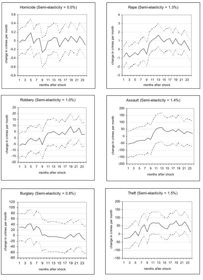
We begin by looking at the effect of monetary policy on broad crime categories (Figure 3): In the Uniform Crime Reports, these categories are: homicide, rape, robberies, assaults, burglaries, and theft. Since the calendar dummies are not of interest, we report only coefficients for the monetary policy regressors. While in all six cases, most coefficients are positive, there are statistically significant lags only in the case of rape and theft. The largest and most statistically significant coefficients occur around or after the 1-year mark, when interest rate policy, according to most economists, begins to have its strongest impact on the economy.
To make the results across crimes comparable, we calculated semi-elasticities of the crime rates with respect to the interest rate, which are also reported in Figure 3. These semi-elasticities are the percent change in the average crime rate over the entire two years, where the numerator in the average equals the mean coefficient estimate of the m
t ˆ−λ
ε regressors, and the denominator is the mean monthly crime rate per : In the case of theft—the crime with the largest
interest semi-elasticity—the results imply that in the two years after a 1% rise in the interest rate, the rate of theft rises 1.5 percent, or about 425 more thefts per million Americans per year.
Also, the Durbin-Watson statistics (not reported here) indicate that residuals are strongly positively autocorrelated. This autocorrelation does not change the unbiasedness of the coefficient estimates. This unbiasedness result follows from the fact that we are running a short regression, omitting other shocks that are uncorrelated with the monetary policy shocks. However, to insure the stability of the results, all reported regressions were also run with AR(1) error structures, with no material change in coefficient sizes or statistical significance.
Given that the largest semi-elasticity was for an economic crime—theft—it is surprising that no statistically significant result was uncovered for robbery. Perhaps this is because aggregation across types of robberies blurs an underlying relationship between monetary policy and the propensity to rob. Accordingly, in Figure 4, we estimated identical regressions, using Uniform Crime Report data on robberies committed with guns, with knives, with other weapons, and with no weapon at all (so-called “strong-arm robberies”). Interest rates appear to have their strongest and statistically most significant impact on knife robberies, with a two-year average semi-elasticity of 2.3%. This implies 6 more knife robberies per million persons per year
Overall, these results support the commonsense hypothesis than when times turn bad, some people turn to crime. But of course, they indicate more than just that. The results indicate that people tend to turn to convenient crimes that promise quick financial gains: Knife robberies and theft. Burglary, a more complicated crime, and gun-assisted robbery, which typically would require the perpetrator to invest in a handgun, do not exhibit the sizable elasticities of more convenient crimes. The statistically significant and relatively large semi-elasticity of rates of rape we cannot explain, and leave to future researchers.
V. Policy Implications and Conclusion
Criminals respond to monetary policy: In particular, we have built upon the vector autoregression framework to show that rates of knife robbery, theft, and rape rise by socially and statistically significant amounts after the Federal Reserve tightens interest rates. How should this result influence monetary policy? In the optimal monetary policy literature, it is well-established that a central bank should reduce the variance of output and of inflation. More controversial has
been the suggestion that the central bank should reduce the variance of interest rates, via interest rate smoothing; this despite the fact that numerous studies (e.g., Taylor, Monetary Policy Rules (2001)) have demonstrated that the Federal Reserve does, in fact, tend to smooth out changes in interest rates.
Our work, demonstrating a link between the volatility of interest rates and the volatility of crime rates, helps establish a socially-motivated reason for such interest-rate smoothing. If governments and private agents face convex adjustment costs of responding to crime rates, then stable crime rates are preferable to more volatile crime rates. For example, if police services move directly with crime rates (via higher caseload, longer hours, etc.), and if police services have an average cost curve with positive first and second derivatives, then police services will be more costly, on average, when crime rates are more volatile.
These results indicate that stable monetary policy has potential social benefits that extend far beyond the traditional macroeconomist’s discussion of unemployment rates and menu costs of inflation. By helping to stabilize crime rates, stable monetary policy can help contribute to social welfare in ways that are only beginning to be explored.
References
Becker, Gary, “Crime and Punishment: An Economic Approach,” Journal of Political Economy 76:2 (1968), 169-217.
Brunner, Alan, “On the Derivation of Monetary Policy Shocks: Should We Throw the VAR Out with the Bath Water?”Journal of Money, Credit, and Banking 32:2 (2000), 254-79.
Christiano, Lawrence, and Martin Eichenbaum, and Charles L. Evans, 1999. “Monetary Policy Shocks: What Have we Learned and What End?” in John B. Taylor and Michael
Woodford, eds., Handbook of Macroeconomics, v. 1A, 64-148.
Ehrlich, Isaac, “Participation in Illegitimate Activities: A Theoretical and Empirical Investigation,” Journal of Political Economy 81:3 (1973), 521-565.
Ehrlich, Isaac, “On the Usefulness of Controlling Individuals: An Economic Analysis of
Rehabilitation, Incapacitation, and Deterrence,” American Economic Review (June 1981), 307-322.
Ehrlich, Isaac, “Crime, Punishment, and the Market for Offenses,” Journal of Economic Perspectives 10 (Winter 1996), 43-68.
Freeman, Richard B., “Why Do So Many Young American Men Commit Crimes and What Might We Do About It?” Journal of Economic Perspectives 10 (Winter 1996), 25-42.
Freeman, Richard B., “The Economics of Crime” Handbook of Labor Economics, vol. 3, (chapter 52 in O. Ashenfelter and D. Card (Eds.), Elsevier Science, 1999).
Goldberger, Arthur S., 1991. A Course in Econometrics. Cambridge, MA: Harvard UP.
Gould, Eric D., Bruce A. Weinberg, and David B, Mustard, “Crime Rates and Local Market Opportunities in the United States: 1979-1997,” Review of Economics and Statistics 84(1) (February 2002), 45-61.
Grogger, Jeff, “Market Wages and Youth Crime,” Journal of Labor and Economics 16:4 (1998), 756-791.
Hamilton, James D. Time Series Analysis. Princeton, NJ: Princeton University Press, 1992
Imrohoroğlu, Ayse, Antonio Merlo, and Peter Rupert, “What Accounts for the Decline in Crime?,” Working Paper No. 01-012, Department of Economics, University of Pennsylvania.
Levitt, Steven, “Using Electoral Cycles in Police Hiring to Estimate the Effect of Police on Crime,” American Economic Review 87 (June 1997), 270-290.
Figure 1
Crimes per Month per Million Americans
1 10 100 1000 10000 1-75 1-76 1-77 1-78 1-79 1-80 1-81 1-82 1-83 1-84 1-85 1-86 1-87 1-88 1-89 1-90 1-91 1-92 1-93 Larceny-Theft Burglaries Assaults All Robberies Rape Homicide
Figure 2
Robberies per Month per Million Americans by type
0 20 40 60 80 100 120 140 1-75 1-76 1-77 1-78 1-79 1-80 1-81 1-82 1-83 1-84 1-85 1-86 1-87 1-88 1-89 1-90 1-91 1-92 1-93 Knife-Cutting Instrument Firearm Strong-Arm Other Weapon
Figure 3 – The response of crime to interest rates: Main Crime Categories Homicide (Semi-elasticity = 0.0%) -0.8 -0.6 -0.4 -0.2 0 0.2 0.4 0.6 1 3 5 7 9 11 13 15 17 19 21 23 months after shock
ch ang e i n c rim es p er mon th Robbery (Semi-elasticity = 1.0%) -20 -15 -10 -5 0 5 10 15 20 25 1 3 5 7 9 11 13 15 17 19 21 23 months after shock
ch an ge in c rim es p er mon th Rape (Semi-elasticity = 1.3%) -3 -2 -1 0 1 2 3 4 1 3 5 7 9 11 13 15 17 19 21 23 months after shock
ch an ge in c rim es p er mo nt h Assault (Semi-elasticity = 1.4%) -200 -150 -100 -50 0 50 100 150 200 1 3 5 7 9 11 13 15 17 19 21 23 months after shock
ch an ge in c rim es p er mo nt h Burglary (Semi-elasticity = 0.8%) -80 -60 -40 -20 0 20 40 60 80 100 120 1 3 5 7 9 11 13 15 17 19 21 23 months after shock
ch ang e i n c rim es p er mon th Theft (Semi-elasticity = 1.5%) -150 -100 -50 0 50 100 150 200 1 3 5 7 9 11 13 15 17 19 21 23 months after shock
ch an ge in c rim es p er mo nt h
Figure 4 – The response of crime to interest rates: Robbery
Firearm Robbery (Semi-elasticity = 1.3%)
-15 -10 -5 0 5 10 1 3 5 7 9 11 13 15 17 19 21 23 months after shock
ch an ge in c rim es p er m ont h
Knife/Cutting Instrument Robbery (Semi-elasticity = 2.3%) -1 -0.5 0 0.5 1 1.5 2 1 3 5 7 9 11 13 15 17 19 21 23
months after shock
ch ang e i n c rim es p er mon th
Other Dangerous Weapon Robbery (Semi-elasticity = 2.0%) -2 -1.5 -1 -0.5 0 0.5 1 1.5 2 1 3 5 7 9 11 13 15 17 19 21 23 months after shock
ch an ge in c rim es pe r m ont h
Strong-arm Robbery (Semi-elasticity = 1.9%)
-8 -6 -4 -2 0 2 4 6 8 10 1 3 5 7 9 11 13 15 17 19 21 23
months after shock
ch ang e i n c rim es p er mon th
Notes: Y-axis values are crimes per month per million Americans. Dashed lines represent +/-2 s.e. bands. The reported semi-elasticity is the mean coefficent value divided by the mean crime rate over the entire sample.
DAVIDSON INSTITUTE WORKING PAPER SERIES - Most Recent Papers
The entire Working Paper Series may be downloaded free of charge at: www.wdi.bus.umich.eduCURRENT AS OF 5/12/04
Publication Authors Date
No. 694: Volatile Interest Rates, Volatile Crime Rates: A New
Argument for Interest Rate Smoothing Garett Jones and Ali M. Kutan May 2004
No. 693 Money Market Liquidity under Currency Board – Empirical Investigations for Bulgaria
Petar Chobanov and Nikolay Nenovsky
May 2004 No. 692: Credibility and Adjustment: Gold Standards Versus Currency
Boards Jean Baptiste Desquilbet and Nikolay Nenovsky May 2004
No. 691: Impact of Cross-listing on Local Stock Returns: Case of
Russian ADRs Elena Smirnova May 2004
No. 690: Executive Compensation, Firm Performance, and State Ownership in China:Evidence from New Panel Data
Takao Kato and Cheryl Long May 2004
No. 689: Diverging Paths: Transition in the Presence of the Informal
Sector Maxim Bouev May 2004
No. 688: What Causes Bank Asset Substitution in Kazakhstan?
Explaining Currency Substitution in a Transition Economy Sharon Eicher May 2004
No. 687: Financial Sector Returns and Creditor Moral Hazard: Evidence from Indonesia, Korea and Thailand
Ayse Y. Evrensel and Ali M. Kutan
May 2004 No. 686: Instability in Exchange Rates of the World Leading
Currencies: Implications of a Spatial Competition Model Dirk Engelmann, Jan Hanousek and Evzen Kocenda May 2004
No. 685: Corporate Spinoffs, Privatization, and Performance in
Emerging Markets Jan Svejnar, Evzen Kocenda and Jan Hanousekf May 2004
No. 684: CPI Bias and Real Living Standards in Russia During the
Transition John Gibson, Steven Stillman and Trinh Le May 2004
No. 683: Mission Implausible III: Measuring the Informal Sector in a
Transition Economy using Macro Methods Jan Hanousek and Filip Palda May 2004
No. 682: The Other Side of the Moon: The Data Problem in Analyzing Growth Determinants
Jan Hanousek, Dana Hajkova and Randall K. Filer
May 2004 No. 681: Consumers' Opinion of Inflation Bias Due to Quality
Improvements Jan Hanousek and Randall K. Filer May 2004
No. 680: IMF-Related Announcements, Fundamentals, and Creditor
Moral Hazard: A Case Study of Indonesia AyKutan şe Y. Evrensel and Ali M. May 2004
No. 679: Privatization Matters: Bank Efficiency in Transition Countries John P. Bonin, Iftekhar Hasan and
Paul Wachtel Apr. 2004
No. 678: Does Market Liberalisation Reduce Gender Discrimination?
Econometric Evidence from Hungary, 1986—1998 Dean Jolliffe and Nauro F. Campos Apr. 2004
No. 677: Governance and Performance of Microfinance Institutions in Central And Eastern Europe and the Newly Independent States
Valentina Hartarska Apr. 2004
No. 676: Equilibrium Exchange Rates in the Transition: The Tradable
Price-Based Real Appreciation and Estimation Uncertainty Balázs Égert and Kirsten Lommatzsch Apr. 2004
No. 675: Productivity growth and the real appreciation of the accession
countries' currencies Kirsten Lommatzsch and Silke Tober Apr. 2004
No. 674: Exchange Rate Policy and Inflation in Acceding Countries: The Role of Pass-through
Fabrizio Coricelli, Boštjan Jazbec and Igor Masten
Apr. 2004
No. 673: Is Kazakhstan a Market Economy Yet? Getting warmer…. Sharon Eicher Apr. 2004
No. 672: Financial Institutions and The Wealth of Nations: Tales of
Development Jian Tong and Chenggang Xu Apr. 2004
No. 671: Interest Rate Pass-Through in EU Acceding Countries: The
Case of the Czech Republic, Hungary and Poland Jesús Crespo Cuaresma, Balázs Égert, and Thomas Reininger Mar. 2004
No. 670: A minimum of rivalry: evidence from transition economies on
the importance of competition for innovation and growth Wendy Carlin, Mark Schaffer and Paul Seabright Mar. 2004
No. 669: Dual Track Liberalization: With and Without Losers Jiahua Che and Giovanni