UNCECOMP 2017 2ndECCOMAS Thematic Conference on Uncertainty Quantification in Computational Sciences and Engineering M. Papadrakakis, V. Papadopoulos, G. Stefanou (eds.) Rhodes Island, Greece, 15–17 June 2017
ROBUST ARTIFICIAL NEURAL NETWORK FOR RELIABILITY
ANALYSIS
Uchenna Oparaji1,2, Rong-Jiun Sheu2, and Edoardo Patelli1
1Institute for Risk and Uncertainty, University of Liverpool
Chadwick Building, Peach Street, Liverpool L69 7ZF, United Kingdom e-mail:{u.oparaji, epatelli}@liverpool.ac.uk
2Institute of Nuclear Engineering and Science
National Tsing Hua University, Hsinchu, Taiwan e-mail:{rjsheu}@mx.nthu.edu.tw
Keywords: Artificial Neural Network, Uncertainty Quantification, Reliability Analysis.
Abstract. Artificial Neural Networks (ANN) are used in place of expensive models to reduce the computational burden required for reliability analysis. Often, ANNs with selected archi-tecture are trained with the back-propagation algorithm from few data representatives of the input/output relationship of the underlying model of interest. However, different performing ANNs might be obtained from the same training data, leading to an uncertainty in selecting the best performing ANN. On the other hand, using cross-validation to select the best performing ANN based on the highest R2value can lead to a biassing in terms of the prediction made by the selected ANN. This is due to the fact that the use of R2cannot determine if the prediction made by ANN is biased. Additionally, R2does not indicate if a model is adequate, as it is possible to have a low R2for a good model and a high R2for a bad model. Hence we propose an approach to improve the prediction robustness of an ANN based on coupling Bayesian framework and model averaging technique into a unified framework. The model uncertainties propagated to the robust prediction is quantified in terms of confidence intervals. Two examples are used to demonstrate the applicability of the approach
©2017The Authors. Published by Eccomas Proceedia.
Peer-review under responsibility of the organizing committee of UNCECOMP2017.
1 INTRODUCTION
Nowadays, numerical models are increasingly used to analyze and predict the performance of complex critical systems. Concurrently, engineering practitioners are concerned with un-certainty, which is inherent to these systems. As a consequence, probabilistic analyses, such as reliability analysis [1], robust design optimization [2], and sensitivity analysis [3], have received much attention in the last decades. However, the computational cost required for performing the aforementioned analyses depends on several factors such as: the numerical model repre-senting the system, the type of analysis, and the treatment of uncertainties (i.e. aleatory and/or epistemic uncertainty). In the context of reliability analysis, the propagation of parameter un-certainties from model inputs to outputs is performed by means of Monte Carlo simulation based approaches. These simulation approaches include: Monte Carlo (MC) [4], and advanced MC such as: Importance Sampling [5], Directional Sampling [6], Line Sampling [7], Subset Simulation [8] etc. Although, advanced MC methods are very efficient, the computational cost required to perform reliability analysis is usually expensive. A popular strategy to reduce the computational costs is to replace the real model with a surrogate model such as an artificial neural network (ANN). ANNs can be constructed based on few data sets from the underlying model of interest. On the other hand, the use of an ANN for this kind of analysis introduces model selection uncertainty in addition to biassing and variance in the estimated quantity of interest. As a matter of fact, an ANN with a specific architecture trained repeatedly with a fi-nite data setDtrain(x,y)results to different performing ANNs whose cost functions are being trapped at different local minima of the cost function solution space. This phenomenon occurs as a result of the random initialization of the weights within each ANN. Consequently, it is of common practice to select the best ANN from the uncertain set on the basis of performance on an independent validation set, and to keep only the network with the lowest validation error and discard the rest. However, there are two disadvantages to such approach. Firstly, all of the effort required to train the remaining networks is wasted. Secondly, the generalization performance of the networks on the validation set has a random component due to the noise on the data, hence the network which had the lowest error on the validation set might perform poorly on a new test set. These disadvantages can be overcome by combining the networks together to form a committee that can significantly improve the robustness of the predicted quantity. Hence, in this paper an approach is proposed to improve the robustness of a neural network when used to predict the probability of failure pF. The outline of this paper is as follows: In Section 2, a succinct theory of reliability analysis using simulation approach and neural network modelling is discussed. This is followed by the proposed approach (Section 3). Next, to demonstrate the applicability of the proposed approach, two numerical examples are tested in Section 4. Finally, conclusions are provided in Section 5.
2 RELIABILITY ANALYSIS
The limit-state function can simply be defined as a deterministic mapping from thez-dimensional input space to a one-dimensional output space:
G:x2Dx⇢Rz!y=G(x)2R (1)
where x is the z-dimensional state variables and y the performance variable. G(x) indicates
if a realization x2Dx corresponds to the safe state (G(x)>0) or failed state (G(x)0). In
realizationx2Dxcorresponds to a failed state in terms of the limit-state functionG(x): pF =P(G(x)0) =
Z
Df fX(x)dx (2) where Df =x2Dx:G(x)0 is the failure region and fX(x) is the joint probability density function of the state variablesX. As Eq.(2) is analytically intractable due its multidimensional nature, Monte Carlo simulation (MCS) (see [4]) allows on to numerically compute the estimate of the failure probabilitypF, considering a large sample of sizeN:
ˆ pF = N1 N
Â
i=1 IG(x)0(xi) (3)whereIG(x)0is the indicator function for failure such thatI=1 forG(x)0 andI=0
other-wise.
2.1 MODELLING ARTIFICIAL NEURAL NETWORK FOR RELIABILITY ANALY-SIS
A setback on the use of MCS to compute the estimate of pF is the large number of model
evaluation required for computing a robust estimate. Hence, an ANN can be used in place of the limit state function to reduce the computational cost. The construction an ANN requires a set of real-valued input/output data pairsDtrain(x,y)of sizeNtraingenerated according to a signal plus noise modely=µ(x) +e, where yis the observed performance generated from the expensive
model,xis the independent state variables sampled from a joint probability densityW(x), e is
independent, identically distributed (iid) noise sampled from a density Y(e) (not necessarily
Gaussian) having mean of 0 and variance s2, and µ(x) the unknown function that is needed
to be approximated by finding an approximation ˆµ(x)from Dtrain(x,y). A priori assumptions can be made about the functional form of µ(x). However, since a parametric function class
is usually unknown, parametric regression approach must be resorted to. Using the non-parametric approach, one constructs an estimate ˆµ(x)of µ(x)from a large class of functions
°known to have good approximation properties. The class of approximation functions usually contains a set of estimators f(w,x)⇢°for which the elements of each subclass f(w,x)are
con-tinuously parametrized by a set of pweightswa;a =1,2, ...,p. The gradient decent algorithm
[9] which is used to minimize the cost functionJof the neural network defined as:
J= 1 Ntrain Ntrain
Â
i=1 (yi yˆi)2 (4)by finding a set of weights wa such that for any given input, the cost function is sufficiently small. However, a limitation of the gradient decent algorithm to train an ANN is the possibility of the cost function to be trapped in a local minimum, thereby reducing the predictive capability of the network.
3 THE PROPOSED APPROACH
The proposed approach aims towards improving the robustness of the prediction made by an ANN when used to perform reliability analysis [10]. The underlying idea behind the proposed approach is to construct a set of ANNs with the same architecture and based on the same training data setDtrain(x,y). By doing so, a distribution of identical ANNs having their error functions
trapped in different local minima is created. The major highlight of this approach is that the solution space of the error function is exploited as many times as possible with the possibility of locating a global minima on the error surface. Further, Bayes’ theorem is used to evaluate the posterior probability of each of the trained ANN based on their likelihood to predict the training data. This is followed by the use of a model averaging technique (adjustment factor approach see [11]) to combine the total prediction made by all the ANNs in the set to yield a robust prediction that converges to the true value. Finally, the model uncertainty propagated to the predicted quantity is quantified in terms of confidence intervals.
3.1 BAYESIAN MODEL SELECTION FOR ARTIFICIAL NEURAL NETWORK
Given a set ofMidentical (i.e. the same model structure) competing ANNsNk,k=1,2, ...M
trained with same data set Dtrain(x,y), Bayes theorem can be used to express the posterior probability of thekthANN in the set which is defined by:
P(Nk|Dtrain) = P(Dtrain(x,y)|Nk)P(Nk)
ÂMq=1P(Dtrain(x,y)|Nq)P(Nq) (5) whereP(Dtrain(x,y)|Nk)is the likelihood of training dataDtrain(x,y)for theNkANN, andP(Nk) is the prior probability ofNk, which is the ANN probability evaluated before observing training dataDtrain(x,y). The prior ANN probabilityP(Nk)can be specified depending on the existing prior knowledge about the credibility of ANNNk, or it can be given as a uniform probability,
P(Nk) =1/M, if no additional information is provided. The advantage of assigning uniform prior probability toP(Nk)is that the difficulty of estimating the prior probability numerically is avoided. The likelihoodP(Dtrain(x,y)|Nk)may be thought of as the probability of observing the training dataDtrain(x,y)underNkANN. It supplies a relative measure of how well theNkANN is supported by the training dataDtrain(x,y). Since the denominator in Eq.(5) is common for all the ANNs, the posterior ANN probability is proportional to prior probability and the likelihood. The likelihood of each ANN is evaluated by measuring the degree of agreement between the training dataDtrain(y)and the response ˆyfor each ANN. Hence, a probabilistic relationship be-tween training dataDtrain(x,y)and ANN predictions ˆyinvolving uncertainty can be described. Typically, the bias function and noise are included as parts of the probabilistic relationship to match ANN predictions with training data. The bias function captures the discrepancies be-tween the expensive model responses and predictions made by the ANN. The noise is usually assumed to be independent and identically distributed normal random variable with a mean of zero [12]. Various authors, see e.g. [13, 14, 15] have used the Bayesian statistical methodol-ogy to quantify the uncertainty in the bias function modelled as a Gaussian process. In their works, a mathematical formulation that combines bias function associated with the ANN and noise from training data is utilized to describe the probabilistic relationship between the train-ing dataDtrain(x,y)and ANN predictions ˆy. The mathematical formulation of this probabilistic relationship is given by the following equation:
Dtrain(y) =yˆ e (6) wheree is a random variable that covers both bias associated with the ANN prediction ˆyand the noise in the response training dataDtrain(y). e is assumed to be an independent identically distributed random variable with a meanµ of zero. The use ofe with zero mean does not shift ANN prediction ˆy. This reflects the fact that ˆy is the most probable prediction value for the ANN. The bias function is not included as a separate term in the probabilistic relationship. This
is due to the fact that introducing a separate bias function results in shifting the prediction ˆyof the ANN from the initially predicted value.
The likelihood P(Dtrain(x,y)|Nk) of training data Dtrain(x,y) for ANN Nk is evaluated by observing where the training data points Dtrain(y) are located in the distribution of ˆy esti-mated by Nk. The procedures to estimate the distribution P(yˆ|Nk) of Nk and the likelihood
P(Dtrain(x,y)|Nk)is given. First, the uncertainty in errors of predictions ˆymade byNk is quan-tified by introducing an assumption that the prediction errors are independent and identically distributed normal random variable with a meanµ of zero. The error of the prediction of thekth network is represented by the following:
eki=Dtrain(yi) yˆi,ekisN(0,sk2),i=1,2, ...,N (7) where Dtrain(yi) is the ith training response output data, ˆyi the prediction of the training data made by Nk, s2
k is the variance of prediction error eki, and N the number of samples in the training data. The prediction error eki measured is considered to be a random sample from a normal distribution with a mean µ of zero and variance s2
k. Using the principle of maximum likelihood estimation (MLE) (see [16]), the variances2
k forNk can be estimated as:
s2 k = N1 N
Â
i=1 e2 ki (8)Secondly, the predictive distributionP(yˆ|Nk)of response ˆyunder modelNkis created by includ-ing the prediction error obtained in the previous step into the prediction of ˆymade byNk. This predictive distribution is defined by the following equation:
P(yˆ|Nk) =Dtrain(y) +eki (9) Lastly, assuming that the residuals between the training dataDtrain(x,y)and ANNNkoutput ˆy are normally and independently distributed with a mean of zero and constant variances2
k, the likelihood functionP(Dtrain(x,y)|Nk)is approximated by:
P(Dtrain(x,y)|Nk)⇡ q 1 2ps2 k 1 N N
Â
i=1 exp{ [yi yˆki] 2 2s2 k } (10)3.2 ROBUST ARTIFICIAL NEURAL NETWORK PREDICTION
To obtain a robust prediction from an ANN, the estimates made by all the subsequent trained ANNs are combined using model averaging technique. Specifically, the adjustment factor ap-proach (see [11]) which is a model averaging technique is combined with Bayes’ theorem. In this way, the ANN having the highest posterior probability is used in conjunction with other respective ANNs trained to correct the bias estimate predicted by the single ANN. The adjust-ment factorAf is evaluated by assuming the error between the prediction of all the subsequent trained ANNs and the training data are normally distributed. The robust ANN prediction can be obtained from the following equation:
yrobust =yˆ⇤+Af (11) where ˆy⇤ represents the point estimate of the best ANN in the set characterised by the highest
Since the adjustment factorAf is assumed to be a normal distribution, the expected value and variance of the adjustment factorAf is given by the following relationships:
E(Af) = M
Â
k=1 P(Nk|Dtrain)(yˆk yˆ⇤) (12) Var(Af) = MÂ
k=1 P(Nk|Dtrain)(yˆk E(yrobust))2 (13) Similarly, the expected value and variance of the robust predictionyad j can be estimated from the following relationships:E(yrobust) =yˆ⇤+E(Af) (14)
Var(yrobust) =Var(Af) (15) whereE(Af)andVar(Af)represents the expected value and variance of the adjustment factor, andE(yrobust)andVar(yrobust)represents the expected value and variance of the robust estimate.
3.3 CONFIDENCE INTERVAL FOR ROBUST ESTIMATE
To quantify the uncertainty in the robust prediction yrobust due to model uncertainty, confi-dence intervals are established. In particular, the 5thand 95thpercentiles of the robust prediction are used quantify the model uncertainty. In theory, this interval is likely to contain the true esti-mated value. As the model uncertainty is assumed to follow normal distribution, the confidence intervals (see [17]) are calculated from the following equations:
CI =E(yrobust) +z⇤pVar(yrobust) (16)
CI =E(yrobust) z⇤pVar(yrobust) (17) whereCI and CI represents the upper and lower confidence intervals of the robust estimate and z⇤ represents the upper critical value of the Gaussian distribution quantifying the model
uncertainty.
4 NUMERICAL EXAMPLE 4.1 THE HAT FUNCTION
The hat function is defined by the analytical expression [18]:
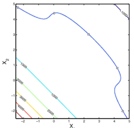
G(x) =20 (x1 x2)2 8(x1+x2 4)3 (18)
wherexi,i=1,2 is defined as Gaussian variables with mean µxi =0.5 and standard deviation
sxi=1.0. Failure is defined asG(x)0 hence pF =P(G(x))0. The limit state surface plot of the hat function is shown in Fig. 1.
−1000 0 0 0 0 0 1000 1000 2000 2000 3000 4000 X1 X2 −2 −1 0 1 2 3 4 5 −2 −1 0 1 2 3 4 5
Figure 1: Limit State Surface of Hat Function
The aim of this example is to verify the proposed approach by replacing the limit state func-tion with an ANN, then compute a robust estimate of ˆpF, quantify the model uncertainty and, finally, verify the number of identical ANNs that must be trained to attain an optimal robust estimate of ˆpF.
4.2 ANALYSIS 1
Training samples Dtrain(x,y) of size Ntrain =2000 have been generated via Latin hyper-cube sampling (LHS) algorithm[19] from the hat function. Two sets Z1= Nk,k= 1,2, ...M andZ2=Ni,i=1,2, ...M composed ofM=1000 identical ANNs have been trained based on
Dtrain(x,y). Specifically, in the first set (Z1), all the training samples inDtrain(x,y)have been used to train the ANNs to maximize their predictive performances. For the second setZ2, 80%
of the training samplesDtrain have been used to train the ANNs and the remaining 20% used for validation. The network architecture chosen for the ANNs in both sets composed of three hidden layers (2,7,1). Next, the posterior probability of the ANNs in setZ1has been estimated
using Bayes’ formula by assigning uniform prior probabilityP(Nk) =1/M to each ANN. On the other hand, the coefficient of determinationR2for the ANNs in setZ
2 have been estimated
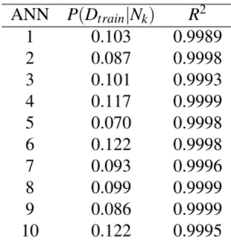
based on the 20% validation samples. Table.1 shows a comparison of 10 selected ANNs from
Z1 and Z2 based on their posterior probabilities and their error values R2. It should be noted
thatith ANN in both set (Z
1andZ2) have been trained inside the same iteration loop, hence the
initialization of the weight values within each loop it is assumed to be similar. Therefore, their resultant performances are expected to be similar. As shown in Table.1, although the ANNs
Ni,i=1,2, ..M in sets Z1 andZ2 are identical as they have been trained in the same iteration
loop, the performance measures in terms of the posterior probability andR2 shows no
agree-ment. For example, the 6th and 10th ANNs have the highest posterior probability, however their correspondingR2 values don’t show a similar trend. Hence, we can support our claim that the
use ofR2value to select the best model is a biased method. Further, to implement the proposed
approach, the ANNs in Z1 have been chosen as they have better performance (i.e. due more
samples used to train them). To accurately compute a robust estimate of ˆpF, 104Monte Carlo simulation runs have been used for each ANN, and the proposed approach presented have been used to average out the prediction made by each ANN model into a robust value that is con-verges to the true value. Finally, the model uncertainty propagated to robust prediction of ˆpF has been quantified in terms of confidence intervals estimated.
ANN P(Dtrain|Nk) R2 1 0.103 0.9989 2 0.087 0.9998 3 0.101 0.9993 4 0.117 0.9999 5 0.070 0.9998 6 0.122 0.9998 7 0.093 0.9996 8 0.099 0.9999 9 0.086 0.9999 10 0.122 0.9995
Table 1: Artificial Neural Networks Posterior Probability Calculated Compared to Correspond-ingR2value.
4.3 ANALYSIS 2
To check the number of ANNs that must be trained in order to obtain a robust value (i.e. close to reference value), the real model has been used to estimate the reference value of ˆpF adopting the same failure criteria (i.eG(x)0) andN=104samples. On the other hand, 3 separate tests
adopting our approach utilizingM = 100, 1000, 10000 identical ANNs respectively have been carried out. As shown in Fig. 2 the robust estimate of ˆpF obtained from the proposed approach converges to the true value (i.e. blue dashed horizontal line) whenM=1000 identical ANNs are
used. This means thatM=1000 ANNs is sufficient enough to explore the entire solution space
of the error function, thus locating a global minima. The importance of this approach is that it can lead to significant improvements in the predictions ˆpF, while involving little additional computational effort. 4 4.5 5 5.5 6 6.5 7 7.5 8 8.5 x 10⁻³ 1 2 3 Failure Probability p F True pF M=100 M=1000 M=10000
(a) 5thand 95thPercentile Confidence Intervals
1 2 3 4 5 6 7 8 9 10 x 10−3 0 50 100 150 200 250 300 350 400 450 500 pF
Probability Density Function
M=100 M=1000 M=10000
(b)Pdf Representing Model Uncertainty
Figure 2: Confidence Intervals and Probability Density Functions Representing Model Uncer-tainty forM=100,1000,10000 Identical Trained Artificial Neural Networks
4.4 CANTILEVER BEAM
A cantilever beam of lengthLand rectangular cross section of widthband heighthis loaded at the end by a concentrated point loadP. The displacementwat the tip of the beam should be
determined for the case where the point loadP, the Young’s modulus E, the density r of the material and the heighthare uncertain.
Figure 3: Cantilever Beam
Uncertainties of the widthband of the lengthLare assumed to be negligible. The
displace-ment w at the tip of the beam where load P is applied can be expressed mathematically as:
w= rgbhL
4
8EI +
PL3
3EI (19)
wheregdenotes gravitational constant, andIis given as:
I= bh
3
12 (20)
The limit state function for the cantilever beam is defined as:
Gcantilever(x) =b w(x) (21)
where b =0.01 is the maximum allowable displacement of the beam. In this example, the
parameter uncertainties are modelled as random variables characterised by probability density function given in Table. 2.
Parameter Distribution µ s SI unit
P Log Normal 5 0.4 KN
h Normal 0.24 0.01 m
r Log Normal 600 140 Kg/m3
E Log Normal 10 1.6 GN/m2
Table 2: Model Input Parameters
The aim of this example is to study how small number of training samples (i.e. Ntrain= 50, 100, 150, 200) affects the robust estimate and the corresponding confidence intervals.
4.5 ANALYSIS 3
In this section, 2 sets (i.e., similar to Section 4.2) of identical ANNs (i.e.M=1000) with
hid-den layer configuration of (4,7,1) have been constructed based onDtrain(x,y),Ntrain= 50, 100, 150, 200 obtained via LHS algorithm [19]. The approach used in Section 4.2 has been adopted here to estimate the posterior probability andR2value of the ANNs. Further, to accurately
com-pute an estimate of ˆpF, 104Monte Carlo simulation runs have been used for each ANN in the first set, and the proposed approach presented have been used to combine the prediction made by each ANN in the first set into a robust ˆpF estimate. Finally, the model uncertainty has been
quantified in terms of confidence intervals of the robust estimate. The results of these analyses are shown in Fig. 4.
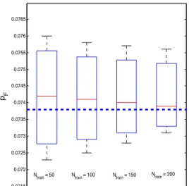
0.0715 0.072 0.0725 0.073 0.0735 0.074 0.0745 0.075 0.0755 0.076 0.0765 1 2 3 4 pF
Ntrain = 50 Ntrain = 100 Ntrain = 150 Ntrain = 200
Figure 4: Robust Confidence Intervals Obtained from Different Number of Training Samples (Ntrain= 50, 100, 150, 200)
Notice that the ”true” (i.e., reference) value of the failure probability (i.e., ˆpF =0.0738, shown in blue dashed lines in Fig. 4) has been obtained with a large number samples (i.e.,
N=104) of simulations of the original model to provide a robust term for comparison. Also,
from the results in Fig. 4, as the number of training samplesNtrain increases, the width of the confidence intervals decreases and the expected value of the robust estimate approaches the reference value (i.e., ˆpF =0.0738). On the other hand, in the cases of small training data sets (e.g.,Ntrain= 50, 100) the failure probabilities are significantly overestimated by the proposed approach (e.g., the expected values of the robust estimate are far off from the reference value) and the associated model uncertainties are quite large. However, in all the cases for small training data sets, the confidence intervals derived is robust enough to capture the true estimate. Hence, in a situation where training data set is small, this approach can be used as a guide to derive a robust confidence interval that is adequate to capture the true value that is being estimated.
5 CONCLUSIONS
Reliability analysis of complex models using the simulation approach is computationally expensive due to the large number of model evaluations required to compute their robust mea-sures. In this paper, an ANN is being used as substitutes for an expensive model to alleviate the computational restrictions. The use of ANN for this kind of analysis introduces additional biasing and variance (i.e uncertainties) to the predicted quantity. It has been shown that the use of cross-validation technique to select the best ANN out of a set of ANN with identical archi-tecture introduces biassing and reduces the robustness of the predicted quantity. Therefore, a novel approach has been presented to enhance the accuracy of the prediction (i.e. robustness) made by an ANN and quantify the model uncertainties in terms of confidence intervals. The proposed approach combines Bayesian model selection and model averaging technique into a unified framework. The applicability of the proposed approach has been demonstrated on two examples. Although the computational effort required for implementing the proposed approach is expensive, parallelization strategies can be adopted to reduce this effort.
Acknowledgements
This work has been partially supported by the EPSRC Grant EP/M018717/1 (Smart on-line monitoring for nuclear power plants (SMART)).
REFERENCES
[1] R. E. Melchers, Structural reliability, Horwood, 1987.
[2] G. Taguchi, Introduction to quality engineering: designing quality into products and pro-cesses, 1986.
[3] I. M. Sobol, Global sensitivity indices for nonlinear mathematical models and their monte carlo estimates, Mathematics and computers in simulation 55 (1) (2001) 271–280.
[4] E. Cashwell, C. Everett, Monte-Carlo methods, Pergamon, London, 1959.
[5] R. Melchers, Importance sampling in structural systems, Structural safety 6 (1) (1989) 3–10.
[6] O. Ditlevsen, P. Bjerager, R. Olesen, A. Hasofer, Directional simulation in gaussian pro-cesses, Probabilistic Engineering Mechanics 3 (4) (1988) 207–217.
[7] M. de Angelis, E. Patelli, M. Beer, Advanced line sampling for efficient robust reliability analysis, Structural Safety 52 (2015) 170–182.
[8] S.-K. Au, E. Patelli, Rare event simulation in finite-infinite dimensional space, Reliability Engineering & System Safety 148 (2016) 67–77.
[9] D. E. Rumelhart, G. E. Hinton, R. J. Williams, Learning internal representations by error propagation, Tech. rep., DTIC Document (1985).
[10] U. Oparaji, R.-J. Sheu, M. Bankhead, J. Austin, E. Patelli, Robust artificial neural network for reliability and sensitivity analysis of complex non-linear systems, Submitted to Neural Networks.
[11] T. Nilsen, T. Aven, Models and model uncertainty in the context of risk analysis, Reliabil-ity Engineering & System Safety 79 (3) (2003) 309–317.
[12] E. Zio, A study of the bootstrap method for estimating the accuracy of artificial neural networks in predicting nuclear transient processes, IEEE Transactions on Nuclear Science 53 (3) (2006) 1460–1478.
[13] M. Bayarri, J. Berger, J. Cafeo, G. Garcia-Donato, F. Liu, J. Palomo, R. Parthasarathy, R. Paulo, J. Sacks, D. Walsh, Computer model validation with functional output, The Annals of Statistics (2007) 1874–1906.
[14] M. J. Bayarri, J. O. Berger, R. Paulo, J. Sacks, J. A. Cafeo, J. Cavendish, C.-H. Lin, J. Tu, A framework for validation of computer models, Technometrics.
[15] M. C. Kennedy, A. O’Hagan, Bayesian calibration of computer models, Journal of the Royal Statistical Society: Series B (Statistical Methodology) 63 (3) (2001) 425–464.
[16] D. G. Kleinbaum, M. Klein, Maximum likelihood techniques: An overview, in: Logistic regression, Springer, 2010, pp. 103–127.
[17] T. H. Wonnacott, R. J. Wonnacott, Introductory statistics, Vol. 19690, Wiley New York, 1972.
[18] B. Sudret, et al., Comparing probabilistic and p-box input modelling in structural reliabil-ity analysis.
[19] J. C. Helton, F. J. Davis, Latin hypercube sampling and the propagation of uncertainty in analyses of complex systems, Reliability Engineering & System Safety 81 (1) (2003) 23–69.