This article was downloaded by: [Bibliotheek TU Delft] On: 04 November 2013, At: 08:09
Publisher: Routledge
Informa Ltd Registered in England and Wales Registered Number: 1072954 Registered office: Mortimer House, 37-41 Mortimer Street, London W1T 3JH, UK
Quantitative Finance
Publication details, including instructions for authors and subscription information: http://www.tandfonline.com/loi/rquf20
Efficient portfolio valuation incorporating liquidity
risk
Yu Tian a , Ron Rood b & Cornelis W. Oosterlee c a
School of Mathematical Sciences , Monash University , Melbourne , VIC , 3800 , Australia
b
RBS—The Royal Bank of Scotland , 280 Bishopsgate, London EC2M 4RB , UK c
CWI—Centrum Wiskunde & Informatica , P.O. Box 94079 , 1090 GB Amsterdam , The Netherlands
Published online: 27 Jun 2013.
To cite this article: Yu Tian , Ron Rood & Cornelis W. Oosterlee (2013) Efficient portfolio valuation incorporating liquidity risk, Quantitative Finance, 13:10, 1575-1586, DOI: 10.1080/14697688.2013.779013
To link to this article: http://dx.doi.org/10.1080/14697688.2013.779013
PLEASE SCROLL DOWN FOR ARTICLE
Taylor & Francis makes every effort to ensure the accuracy of all the information (the “Content”) contained in the publications on our platform. However, Taylor & Francis, our agents, and our licensors make no
representations or warranties whatsoever as to the accuracy, completeness, or suitability for any purpose of the Content. Any opinions and views expressed in this publication are the opinions and views of the authors, and are not the views of or endorsed by Taylor & Francis. The accuracy of the Content should not be relied upon and should be independently verified with primary sources of information. Taylor and Francis shall not be liable for any losses, actions, claims, proceedings, demands, costs, expenses, damages, and other liabilities whatsoever or howsoever caused arising directly or indirectly in connection with, in relation to or arising out of the use of the Content.
This article may be used for research, teaching, and private study purposes. Any substantial or systematic reproduction, redistribution, reselling, loan, sub-licensing, systematic supply, or distribution in any
form to anyone is expressly forbidden. Terms & Conditions of access and use can be found at http:// www.tandfonline.com/page/terms-and-conditions
Efficient portfolio valuation incorporating liquidity
risk
YU TIAN
∗†, RON ROOD‡
and CORNELIS W. OOSTERLEE§
† School of Mathematical Sciences, Monash University, Melbourne, VIC 3800, Australia‡RBS—The Royal Bank of Scotland, 280 Bishopsgate, London EC2M 4RB, UK
§CWI—Centrum Wiskunde & Informatica, P.O. Box 94079, 1090 GB Amsterdam, The Netherlands (Received 21 December 2010; in final form 14 February 2013)
According to the theory proposed by Acerbi and Scandolo (2008) [Quant. Finance, 2008, 8, 681–692], an asset is described by the so-called Marginal Supply–Demand Curve (MSDC), which is a collection of bid and ask prices according to its trading volumes, and the value of a portfolio is defined in terms of commonly available market data and idiosyncratic portfolio constraints imposed by an investor holding the portfolio. Depending on the constraints, one and the same portfolio could have different values for different investors. As it turns out, within the Acerbi–Scandolo theory, portfolio valuation can be framed as a convex optimization problem. We provide useful MSDC models and show that portfolio valuation can be solved with remarkable accuracy and efficiency.
Keywords: Liquidity risk; Portfolio valuation; Ladder MSDC; Liquidation sequence; Exponential MSDC; Approximation
JEL Classification: C60, G11, G12
1. Introduction
According to the theory developed by Acerbi and Scandolo
(2008) the value of a portfolio is determined by market data and a set of portfolio constraints. The market data is assumed to be publicly available and is the same for all investors. The market data consists of price quotes corresponding to different trading volumes. These quotes for an asset are represented in terms of a mathematical function referred to as a Marginal Supply–Demand Curve (MSDC).
The portfolio constraints may vary across different players. These idiosyncratic constraints—collectively referred to as a
liquidity policy—refer to restrictions that any portfolio held by
the investor should be prepared to satisfy. Examples of such portfolio constraints are:
• minimum cash amounts to meet short-term liquidity needs;
• market or credit risk management limits;
• capital limits.
We introduce the fundamental concepts of Acerbi–Scandolo theory in section 2. To value her portfolio, the investor will mark all the positions she could possibly unwind to satisfy the liquidity policy to the best price according to an MSDC ∗Corresponding author. Email: [email protected]
function. As it turns out, within Acerbi and Scandolo’s theory, the valuation of a portfolio of assets can be framed as a convex optimization problem. The associated constraint set is repre-sented by a liquidity policy. Although this was already pointed out by Acerbi and Scandolo themselves, the practical implica-tions of the theory have as yet not been well investigated. Such is the aim of the present paper.
We will study portfolio valuation under theAcerbi–Scandolo theory extensively, assuming different forms of the MSDC function. We first consider a very general setting where the MSDC is shaped as a non-increasing step function (referred to
as aladder MSDC) in section3. This corresponds to normal
market situations for relatively actively traded products such as listed equities. We will present an algorithm for portfolio valuation assuming ladder MSDCs and a cash portfolio con-straint. In section4, we will look at MSDCs that are shaped as decreasing exponential functions, which can be used to describe less-liquid over-the-counter (OTC) traded products. We will also see how the exponential functions can be used as approximations of ladder MSDCs.
All numerical results are collected in section5. We will find that, in a wide range of cases, the approximation of ladder MSDCs by exponential MSDCs appears to be accurate, sug-gesting that not all market price information represented in ladder MSDCs is necessary for accurate portfolio valuation. We present our conclusions in section6.
© 2013 Taylor & Francis
2. The portfolio theory
This section presents relevant concepts and results from Acerbi and Scandolo (2008) that will be used throughout this paper.
2.1. Asset
An assetis an object traded in a market and will be
charac-terized by a Marginal Supply–Demand Curve (MSDC). This codifies available bid and ask prices corresponding to different trading volumes.
Definition 2.1: AnMSDCis a mapm:R\{0} →Rsatisfying the following two conditions:
(1) m(s)is non-increasing, i.e.m(s1)≥m(s2)ifs1<s2; (2) m(s)is càdlàg (i.e. right-continuous with left limits) for s < 0 and làdcàg (i.e. left-continuous with right limits) fors>0.
The variablesrepresents the trading volume of the asset. Condition 1 represents a no-arbitrage assumption. Condi-tion 2 ensures that MSDCs have elegant mathematical proper-ties. We will not use this condition heavily and we only mention it for the sake of completeness. Instead, what we will need most of the time is that an MSDC is (Riemann) integrable on its domain.
We call the limitm+:=limh↓0m(h)thebest bidandm−:=
limh↑0m(h)thebest ask. Thebid–ask spread, denoted byδm,
is defined asδm:=m−−m+.
Definition 2.2: Cash is the asset representing the currency paid or received when trading any asset. It is characterized by a constant MSDC, m0(s) = 1 (i.e. one unit) for every
s∈R\ {0}.
Cash is referred to as aperfectly liquidasset if the associated MSDC is constant. We call asecurityany asset whose MSDC is a positive function (e.g., a stock, a bond, a commodity) and a swapany asset whose MSDC can take both positive and negative values (e.g., an interest rate swap, a CDS, a repo transaction). A negative MSDC can be converted into a security by defining a new MSDC asm∗(s):= −m(−s).
We presuppose one currency as the cash asset. For example, if we choose the euro as the cash asset, relative to the euro, the US dollar will be considered as an illiquid asset.
2.2. Portfolio
A portfolio is characterized by listing the holding volumes of different assets in the portfolio. Given areN+1 assets labeled 0,1, . . . ,N. We let asset 0 label the cash asset.
Definition 2.3: Aportfoliois a vector of real numbers,p =
(p0,p1, . . . ,pN) ∈ RN+1, where pi represents the holding volume of asseti. In particular,p0denotes the amount of cash in the portfolio.
When we specifically want to highlight the portfolio cash we tend to write a portfolio asp = (p0,p). We henceforth presuppose a set of portfolios referred to as theportfolio space
P. We will assume thatPis a vector space so that it becomes
meaningful to add portfolios together and to multiply portfolios by scalar numbers. Letp=(p0,p)∈Pand suppose we have an additional amountaof cash. We writep+a=(p0+a,−→p). Definition 2.4: Theliquidation Mark-to-Market (MtM) value L(p)of a portfoliopis defined as L(p):= N i=0 pi 0 mi(x)dx= p0+ N i=1 pi 0 mi(x)dx. (1)
The liquidation MtM value can be viewed as the value of a portfoliopfor an investor who should be able to liquidate all her positions in exchange for cash.
Definition 2.5: Theuppermost Mark-to-Market (MtM) value U(p)ofpis given by U(p):= N i=0 m±i pi = p0+ N i=1 m±i pi, (2) where m±i = m+i ,ifpi >0, m−i ,ifpi <0. (3)
The uppermost MtM value can be viewed as the value of a portfolio for an investor who has no cash demands. In this sense, the portfolio is unconstrained.
As MSDCs are non-increasing,U(p) ≥ L(p). The differ-ence betweenU(p)andL(p)is termed theuppermost
liquida-tion costand is defined asC(p):=U(p)−L(p).
2.3. Liquidity policy
The definitions of the liquidation MtM value L(p) and the uppermost MtM valueU(p)suggest that the value of a portfolio pis subject to certain cash constraints an investor should be able to meet by wholly or partly liquidating positions she has taken. These constraints are represented as aliquidity policy.
There could be other types of constraints besides. For exam-ple, an investor might want to impose market risk VaR limits on her positions, or credit limits, or capital constraints. All the constraints that an investor imposes can be represented as a subset of the underlying portfolio spaceP. These constraints are collectively referred to as a liquidity policy. We refer to
Acerbi and Finger(2010) andWeberet al.(2013).
Definition 2.6: Aliquidity policyL is a closed and convex subset ofP satisfying the following conditions:
(1) ifp =(p0,p)∈ Landa ≥ 0, thenp+a =(p0+
a,p)∈L;
(2) ifp∈L, then(p0,0)∈L.
Example 2.7: A liquidity policy setting a minimum cash re-quirement,c, is acash liquidity policy:
L(c):= {p∈P|p0≥c≥0}. (4) An investor endorsing a cash liquidity policy should be prepared to liquidate her positions to such an extent that min-imum cash levelcis obtained. We will extensively use cash
liquidity policies in sections3and4. We refer toAcerbi(2008) andWeberet al.(2013) for additional examples of liquidity policies.
2.4. Portfolio value
This section presents Acerbi and Scandolo’s definition of the portfolio value function. We first need the following definition. Definition 2.8: Letp,q ∈ P be portfolios. We say thatqis
attainablefrompifq =p−r+L(r)for somer∈P. The
set of all portfolios attainable frompis written asAtt(p). The following definition is key.
Definition 2.9: TheMark-to-Market (MtM) value(or thevalue, for short) of a portfoliopsubject to a liquidity policyLis the value of the functionVL:P→R∪ {−∞}, defined by
VL(p):=sup{U(q)|q∈Att(p)∩L}. (5)
IfAtt(p)∩L=∅, meaning that no portfolio attainable from psatisfiesL, then we stipulate the portfolio value to be−∞.
Acerbi and Scandolo(2008) give the following proposition of the new portfolio value.
Proposition 2.10: The portfolio value functionVLfrom def-inition 2.9 can be alternatively defined as
VL(p)=sup{U(p−r)+L(r)|r∈P,p−r+L(r)∈L}.
(6) To prove this is not very difficult; we refer to Acerbi and Scandolo (2008).
Proposition 2.10 allows us to frame the determination of the value of a portfolio as an optimization problem with explicit constraints, namely ⎧ ⎨ ⎩ maximize U(p−r)+L(r), subject to p−r+L(r)∈L, r∈P. (7) (We ignore the case VL(p) = −∞.) This optimization problem is convex asLis a convex set. SinceLis also closed, this problem has a unique optimal value (which could be−∞).
3. Portfolio valuation using ladder MSDCs
In the previous section we have outlined the main concepts of Acerbi and Scandolo’s portfolio theory. We discussed that portfolio valuation could be framed as a convex optimiza-tion problem (7). Convex optimization problems can often be solved numerically (Boyd and Vandenberghe,2004).
In the present section we will provide an algorithm providing an exact global solution for problem (7) under the assumption that the MSDC for illiquid assets is piecewise constant; as such we will name themladder MSDCs.
Within the Acerbi–Scandolo theory, ladder MSDCs will play a key role in modeling the liquidity of the assets. Equipped with the fast and accurate algorithm discussed in this section, one could solve the convex optimization problem incurred in portfolio valuation more efficiently than using conventional optimization techniques.
3.1. The optimization problem
Generally we assume a market wherein we can quote a price for each volume we wish to trade, i.e. a market of ‘unlimited depth’. However, in a real-world market context, we will typi-cally only be able to trade volumes within certain bounds. The upper and lower bounds of this domain represent the market depth: the upper bound represents the maximum volume we will be able to sell against prices we can quote from the mar-ket and the lower bound represents the maximum we will be able to buy against prices we will be able to quote from the market.Weberet al.(2013) refer to this set of constraints on the portfolio space as aportfolio constraint. In the context of limited market depth, we will need to restrict the domain to a subset of the portfolio space to solve the optimization problem of portfolio valuation.
In what follows, we still assume unlimited market depth so that we can search for the optimal solution in the whole portfolio space for simplicity, whereas the method we state below also works with limited market depth.
Reconsider problem (7). Using a cash liquidity policyL(c)
this becomes⎧ ⎨ ⎩ maximize U(p−r)+L(r), subject to p0−r0+L(r)≥c, r∈P. (8) The inequality constraint can be replaced by the equality constraint p0−r0+L(r)= cwithout affecting the optimal value of the original problem. Furthermore, we may assume that the cash componentr0equals 0 as it does not play a role in the optimization problem. To find the optimal solution we hence might as well solve
⎧ ⎨ ⎩ maximize U(p−r)+L(r), subject to L(r)=c−p0, r∈P. (9) Note that, without loss of generality, we may assume thatp0= 0; otherwise use the cash liquidity policyL(c−p0).
3.2. A calculation scheme for portfolio valuation with ladder MSDCs
In the case of portfolio valuation based on ladder MSDCs we can solve the associated optimization problem (9) numerically, for example by an interior point algorithm (Boyd and Vandenberghe, 2004). However, the implementa-tion of the algorithm could be computaimplementa-tionally inefficient in the sense that several iterations might be required to bring the solution within reasonable bounds in high dimensions. In ad-dition, the non-smoothness of the ladder MSDCs increases the difficulty of implementing conventional convex optimization algorithms.†Hence, the aim of this section is to provide an algorithm for problem (9) yielding an exact global optimal solutionr∗.
Unless otherwise stated, throughout the remainder of this section we use the following assumption.
†For example, the optimality conditions in the interior point algorithm will not apply at non-smooth points of the ladder MSDC. See Boyd and Vandenberghe(2004) for more information.
Assumption 3.1: Any investor holds a portfoliopconsisting
of long positions only and uses a cash liquidity policy L(c)
(c>0).
Proposition 3.2: Under assumption 3.1, the maximization
problem (9) has the same optimal solution as the following
minimization problem: ⎧ ⎨ ⎩ minimize C(r), subject to L(r)=c−p0, r∈P. (10) Proof: Since we are prepared to liquidate our portfolio for cash under a cash policy, the portfoliospandrshould have the same sign componentwise. It follows that U(p−r) =
U(p)−U(r)by the definition of the uppermost MtM value. Consequently, the objective function of problem (9) can be rewritten as
U(p)−U(r)+L(r).
Since, givenp, we can always determineU(p), maximizing this function under the given constraints will yield the same optimal solutionr∗as maximizing the following function under the same constraints:
−U(r)+L(r). Obviously, minimizing
U(r)−L(r)
again yields the same optimal solutionr∗. Noting thatC(r)=
U(r)−L(r)proves the result.
Remark 1: The following inequality holds in general:
U(p−r)≤U(p)−U(r).
For example, we may be prepared to increase our share in several risky assets or reduce the purchase of risky assets. In situations like these, components of the original portfoliopand corresponding components of to-be-liquidated portfoliormay have different signs. Equality holds under assumption 3.1.
Informally, proposition 3.2 implies that to determine the value of a portfolio under a cash liquidity policy is to determine a portfolio r∗ such that liquidatingr∗ in exchange for cash minimizes the uppermost liquidation cost C(r∗). This result will prove useful at a later stage.
Given that all assets are assumed to be characterized by ladder MSDCs, we can conveniently break up each and every position in our portfolio into a finite number of volumes. To each of these volumes there corresponds a definite market quote as represented by the MSDC.
The idea of the algorithm is to consider all of these portfolio bits together and to liquidate them in a systematic and orderly manner, starting with the portions that will be liquidated with the smallest cost relative to the best bid, and subsequently to those that can be liquidated with the second smallest cost, and so on, until the cash constraint is met.
If the minimum cash requirement that the portfolio should be prepared to satisfy exceeds the liquidation MtM value of the entire portfolio, then we will never be able to meet the cash constraint; by definition, we set the portfolio value to be−∞. Alternatively, suppose that we sell off a fraction of each position against the best bid price and that the total cash we
subsequently receive in return exceeds the cash constraint. Then the value of the portfolio equals the uppermost MtM value and there exist infinitely many optimal solutions.
We will now make this formal, starting with the following definition.
Definition 3.3: Given is an asseti, characterized by MSDC
mi. Theliquidity deviationof a volumesof asseti is defined as
Si(s):=
m+i −mi(s)
m+i , fors>0. (11)
The liquidity deviation is the relative difference between the best bid price and the last market quotemi(s)hit for a volume
s. In this sense, it measures the liquidity of asseti atsi units traded relative to the best bid.
Given any asset, the liquidity deviation is a non-decreasing function, as the MSDC corresponding to that asset is non-increasing. For a security, the values of the liquidity deviation are in[0,1], as the lower bound of the corresponding MSDC is 0. For a swap, the values are in[0,+∞). Since the MSDC of an asset is assumed to be piecewise constant, each value of the liquidity deviation corresponds to a maximum bid size.
Using the previously defined liquidity deviation, positions are liquidated in a definite order, as follows. Given a portfolio r=(r0,r1, . . . ,rN), assume that we want to liquidate all the
ri,i >0. Each non-cash positionri can be written as a sum
ri =
Ji
j=1
ri j, i =1, . . . ,N, (12)
whereri j is called aliquidation size.
To define the liquidation sizeri j, consider the bid part of a ladder MSDCmi, which is constructed by a finite number of bid prices with maximum bid sizes. For eachri in asseti, we can identify a finite numberJiof bid pricesmi jwith liquidation sizesri j, j =1, . . . ,Ji.
For the firstJi−1 liquidation sizesri j(j =1, . . . ,Ji−1), they are equal to the firstJi−1 maximum bid sizes recognized from the market. For theJith liquidation sizeri j, it is less than or equal to theJith maximum bid size. Moreover, each liqui-dation sizeri jcorresponds to each bid pricemi j. In particular, the first liquidation size of each assetri1 corresponds to the best bidm+i =mi1.
The liquidity deviation for each liquidation size can then be written as Si j = m+i −mi j m+i = mi1−mi j mi1 . (13)
Now we put the liquidity deviationsSi j in ascending order indexed by k, and we generically refer to any term of this sequence as Sk(r) (the addition of ras an extra parameter will prove convenient later on). Note that the length of the liquidation sequence equalsK =J1+ · · · +JN.
In addition, we observe that there exists a natural one-to-one correspondence between the sequence{Sk(r)}, the sequence of liquidation size{ri j}and the sequence of bid prices{mi j}. Hence, while preserving these one-to-one correspondences, we relabel the sequences{ri j}and{mi j}as{rk}and{mk}, respec-tively. We call the sorted indexk the liquidation sequence, which is a permutation of the index(i,j).
Table 1. Bid price information of assets 1 and 2.
Maximum bid size Bid price Maximum bid size Bid price
(a) Asset 1 (b) Asset 2
200 11.65 200 19.58
200 11.55 600 19.5
200 11.45 200 19.2
Table 2. Liquidation size of our portfolior=(0,600,900).
Liquidation size Bid price
(a) Asset 1 r11 200 m11 11.65 r12 200 m12 11.55 r13 200 m13 11.45 (b) Asset 2 r21 200 m21 19.58 r22 600 m22 19.5 r23 100 m23 19.2
Table 3. Liquidity deviation and liquidation sequence.
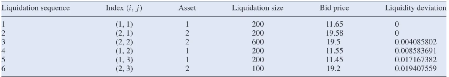
Liquidation sequence Index(i,j) Asset Liquidation size Bid price Liquidity deviation
1 (1, 1) 1 200 11.65 0 2 (2, 1) 2 200 19.58 0 3 (2, 2) 2 600 19.5 0.004085802 4 (1, 2) 1 200 11.55 0.008583691 5 (1, 3) 1 200 11.45 0.017167382 6 (2, 3) 2 100 19.2 0.019407559
Note that the firstNterms of the sequence{mk}are the best bidsm+i ,i =1, . . . ,N.
To illustrate the above concepts, consider an example as follows. Given two illiquid assets, the bid parts that can be read from the market are shown in table1. Assume that we hold a portfolio that contains 600 units in asset 1 and 900 in asset 2. The liquidation sizes for the two assets are shown in table2
and the sorted liquidity deviations as well as the liquidation sequence are presented in table3.
To meet the cash constraint embodied in the cash liquidity policy we start liquidating the portfolio fromS1(r), thenS2(r), and so on, until we have met the cash requirement.
The liquidation sequence effectively directs the search pro-cess throughout the constraint set towards the global solution, and exactly so. This is summarized in the following theorem, which we will prove subsequently.
Proposition 3.4: Given is a portfoliopsuch that each asset is characterized by a ladder MSDC. Under assumption 3.1, the
optimization problem(9)has the same optimal solution as the
following: ⎧ ⎨ ⎩ minimize Kk=1Sk(r), subject to L(r)=c−p0, r∈P. (14)
Loosely put, the optimal solution is the one yielding the min-imum total sum of liquidity deviation. Intuitively, the propo-sition implies that, to meet cash demands, we should liquidate the most liquid assets as they are easier to sell off and their liquidation will incur less losses compared with more illiquid assets.
Proof: Let a portfoliop = (p0,p1, . . . ,pN)be given and suppose we liquidate a portfolior=(r0,r1, . . . ,rN)to meet a liquidity policyL. Asseti has a corresponding MSDCmi,
i =0,1, . . . ,N. For simplicity,r0is set to be 0.
From proposition 3.2, the optimal solution of (9) minimizes the uppermost liquidation cost. Using that all assets are char-acterized by ladder MSDCs, the objective functionC(r)can be rewritten as follows: C(r)=U(r)−L(r) = N i=1 Ji j=1 (m+i ri j−mi jri j).
Note that, for each asseti,m+i ≥mi j for all j. It follows that the minimum of the sum of the absolute differences between
m+i ri j andmi jri j is the same as the minimum of the sum of the relative differences. Hence, to find the optimal solution we might as well minimize
N i=1 Ji j=1 m+iri j−mi jri j m+iri j = N i=1 Ji j=1 m+i −mi j m+i = N i=1 Ji j=1 Si j(r) = K k=1 Sk(r).
On the last line, note thatK =J1+ · · · +JN. Based on this result, we now state the algorithm for portfolio valuation assuming only ladder MSDCs under assumption 3.1. For the sake of clarity we recall that the optimal solutionr∗of problem (9) should satisfyL(r∗)=c−p0. Also, we assume that p0 = 0 and r0 = 0. (Otherwise, we can set the cash requirementc= c− p0.) The pseudocode is summarized in algorithm1.
Algorithm 1: Algorithm for portfolio valuation assuming lad-der MSDCs anda cash liquidity policyL(c)
Calculate: U(p)=iN=1m+i ·pi; L(p)=iN=1Ji j=1mi j ·pi j; V1(p)= N i=1m+i ·pi1; Si j =(mi1−mi j)/mi1;
Sort theSi jas an ascending sequence with indexk. {With k
running from1to J1+ · · · + JN}
ifc>L(p)then
return VL(c)(p)= −∞; {There is no optimal solution
satisfying the cash constraint.}
else
ifc=L(p)then
return VL(c)(p)=L(p); {The optimal solutionr∗= p.}
else
if c ≤ V1(p)then {Liquidating pi1to the respective
best bids meets the cash constraint.}
return VL(c)(p)=U(p); {There are infinitely many
optimal solutions.}
else
U(r)=V1(p);
c=c−V1(p);
k=N+1; {Start loop from the first part with non-zero
liquidity deviation until c becomes 0.}
whilec>0do ifc/mk >pkthen U(r)=U(r)+m+k ·pk; c=c−mk·pk; k=k+1; else U(r)=U(r)+m+k ·(c/mk); c=0; end if end while
return VL(c)(p)=U(p)−U(r)+c{Here we have
L(r)=c.}
end if end if end if
There are generally four cases stated in algorithm1: (1) if the cash requirementcis higher than the liquidation
MtM value L(p) such that the cash liquidity policy cannot be met, then we assign −∞ to the portfolio value VL(c)(p)and conclude that there is no optimal solution;
(2) if the cash requirementcis equal to the liquidation MtM value L(p)such that we have to liquidate all parts of the portfolio, then the portfolio valueVL(c)(p)equals the liquidation MtM valueL(p)and the unique optimal solutionr∗=p;
(3) if the cash requirementcis less than or equal toV1(p), the liquidation value of all parts of the portfolio cor-responding to the best bids, then the portfolio value
VL(c)(p) equals V1(p) and there exist infinite many optimal solutions;
(4) if the cash requirementcis higher thanV1(p)but less thanL(p), we have to liquidate the portfolio along the liquidation sequence until the cash requirement is met and the unique optimal solutionr∗ can be found by recording the liquidation parts of corresponding assets in the calculation procedure of the algorithm.
The piecewise constant MSDCs in the convex optimization problem generally increase the difficulty of the search for the global optimal solution with standard software. With the afore-mentioned calculation scheme listed in algorithm1, instead, we can solve the optimization problem accurately and efficiently via the liquidation sequence.
4. Portfolio valuation using continuous MSDCs
There typically is no analytic solution to the convex optimiza-tion problem (9). However, it can be shown that if we model the MSDC as a continuous function we can obtain simple analytic solutions from the method of Lagrange multipliers. In section4.1we will first look at continuous MSDCs without imposing any specific form for them. We will subsequently look at MSDCs shaped as exponential functions in sections4.2
and 4.3. Empirically, we find that exponential MSDCs can be used to model MSDCs for security-type equity assets with different caps. We then propose to use exponential MSDCs to approximate ladder MSDCs in order to improve the efficiency of portfolio valuation in section4.4. We will assume the cash liquidity policy in this section.
4.1. The general case
Assume N illiquid assets labeled 1, . . . ,N with MSDCsmi,
i =1,2, . . . ,N. Eachmi is assumed to be continuous onR. This implies thatmi(0)exists. We will exclude the pointmi(0) later in this section. In addition, each mi is assumed to be strictly decreasing. Adopting a cash liquidity policy, valuing a portfolio consisting of positions in these assets comes down to solving the optimization problem (9). The solution to this optimization problem can be derived analytically, as is shown by the following proposition proposed byAcerbi and Scandolo
(2008).
Proposition 4.1: Assuming continuous strictly decreasing
MS-DCs and the cash liquidity policyL(c), the optimal solution
r∗ =(0,r∗)to optimization problem(9)is unique and given
by
ri∗= m
−1
i [mi(0)/(1+λ)], if p0<c,
0, if p0≥c, (15)
where m−i 1(·)denotes the inverse of the MSDC function mi(·),
and the Lagrange multiplierλ, representing the marginal
liq-uidation cost, can be determined from the equation L(r∗)=
c−p0.
We refer toAcerbi and Scandolo(2008) for a proof. Remark 2: Note that we can extend the above to the case where the MSDCs are not continuous at the point 0, i.e. the case where there is a positive bid–ask spread. We have to change the definition of the value atmi(0)to the limitm+i in the case of long positions or tom−i in the case of short positions.
Obviously, by using the Lagrange multiplier method, we can generalize the case to any liquidity policy giving rise to equality constraints. When using a general liquidity policy which results in inequality constraints, we can solve the op-timization problem (7) by checking the Karush–Kuhn–Tucker (KKT) conditions. In addition, the Lagrange dual method may also be useful.
4.2. Exponential MSDCs for large- and medium-cap equities
We continue the discussion by looking at a particular example of a MSDC, i.e. the exponential MSDC. As it turns out, the exponential MSDCs form an effective model to characterize a security-type asset and to determine the portfolio value by convex optimization. We will discuss this in section4.4.
Many researches have shown that there is a relation between the price change and the trading volume in the market during a short time period.Contet al.(2011) propose that there is a ‘square-root’ relation between the price change and the trading volume for S&P 500 equities.Almgrenet al.(2005) found a similar result and proposed a ‘3/5’ relation between the tempo-rary price impact and the trade size for large-cap US equites. These parameters correspond to a medium-size price impact.
In our paper, we interpret the price change as log(m(s)/m+), i.e. the relative change between the bid (or ask) pricem(s)and the best bid m+ (or best ask m−) over a short time period, during which an MSDC can be formed and denote the trading volume to bes.
Large- and medium-cap equities listed on stock exchanges such as the London Stock Exchange and Euronext are actively traded and thus relatively liquid. From available data we ob-serve a ‘square-root’ relation between the bid price change and the volume over a short time, as follows:
log m(s) m+ = −k√s+, (16) wherem+,k>0 andis the noise term.
For the ask price part, wheres <0, we have the following model: log m(s) m− =k|s| +, (17) wherem−,k>0 andis the noise term.
When skipping the noise term, we use the following expo-nential MSDC model to approximate the bid part of the ladder MSDC for a large- or medium-cap equity:
m(s)=m+·e−k√s, (18)
and we approximate the ask part as
m(s)=m−·ek√|s|. (19)
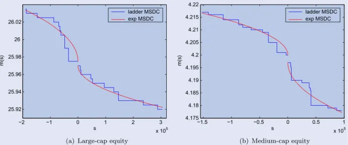
We give two examples of the ladder MSDCs and the above approximated exponential MSDCs by least-squares regression for large- and medium-cap equities in figure1.
Suppose there areN (large- or medium-cap) security-type assets 1,2, . . . ,N, the bid parts of which are characterized by
mi(s)=m+i ·e−ki
√
s. (20)
We callki the liquidity risk factor for the corresponding asseti (i =1, . . . ,N), which measures the general liquidity condition of asseti. From proposition 4.1 and remark2, we can approximate portfolio values under different liquidity policies. As an example, assuming a portfolio with only long posi-tions, then we have the liquidation MtM value
L(p) = p0+ N i=1 pi 0 mi(x)dx = p0+ N i=1 2m+i k2i (1−ki √ pie−ki √p i−e−ki√pi), (21) and under a cash liquidity policy L(c)with p0 < c, from proposition 4.1, we have ri∗= log(1+λ) ki 2 , i=1, . . . ,N, withλ=ex−1, x>0, and 1−Nc−p0 i=1(2m+i /k2i) ex−x−1=0. (22)
The last equation can be solved numerically by using the Newton–Raphson iteration method or the Taylor’s expansion. Hence, the portfolio value under the cash liquidityL(c)reads
VL(c)(p) =U(p−r∗)+L(r∗) = N i=1 mi+· pi − log(1+λ) ki 2 +c.(23) For large- and medium-cap assets, since they are generally very liquid to trade, the uppermost liquidation cost is usually very small.
4.3. Exponential MSDCs for small-cap equities
On the other hand, for small-cap equities, we find there is a ‘square’ relation between the bid price change and the volume over a short time, which implies a large price impact:
log m(s) m+ = −ks2+, (24) wherem+,k>0 andis the noise term.
−2 −1 0 1 2 3 x 10⁵ 25.92 25.94 25.96 25.98 26 26.02 s m(s) ladder MSDC exp MSDC −1.5 −1 −0.5 0 0.5 1 x 10⁵ 4.175 4.18 4.185 4.19 4.195 4.2 4.205 4.21 4.215 4.22 s m(s) ladder MSDC exp MSDC
Figure 1. Exponential MSDCs versus ladder MSDCs for large- and medium-cap equities.
Similarly, for the ask price change we have log m(s) m− =k|s|2+, (25) wherem−,k>0 andis the noise term.
When skipping the noise term, we have the following expo-nential MSDC model to approximate the bid part of a ladder MSDC of a small-cap equity:
m(s)=m+·e−ks2, (26)
and for the ask part we have the exponential MSDC
m(s)=m−·ek|s|2. (27)
We give an example of a ladder MSDC and the approximated exponential MSDC for a small-cap equity in figure2.
Suppose that there are N (small-cap) security-type assets 1,2, . . . ,N, whose bid parts are characterized by the following exponential MSDCs:
mi(s)=m+i ·e−
kis2, (28) withm+i ,ki >0 for alli=1, . . . ,N. By using a least-squares approximation, we can fit the value ofm+i andki from real data. See section4.4.
To illustrate this type of exponential MSDC function, we as-sume a portfolio with only long positions. Then the liquidation MtM value reads L(p) = p0+ N i=1 pi 0 mi(x)dx = p0+ √ π 2 N i=1 m+i √ ki · erf(kipi), (29)
where erf(·)is the Gauss error function, which can be obtained numerically. −2 −1 0 1 2 x 10⁶ 1.4 1.45 1.5 1.55 1.6 s m(s) ladder MSDC exp MSDC
Figure 2. Exponential MSDCs versus ladder MSDCs for a small-cap equity.
For a cash liquidity policyL(c)withp0<c, from proposi-tion 4.1 we have ri∗= log(1+λ) ki , i =1, . . . ,N, withλ=ez2−1, (30) z=erf−1 c−p0 (√π/2)iN=1(mi+/√ki) ,
where erf−1(·)is the inverse error function, which can also be obtained numerically. Hence,
VL(c)(p) =U(p−r∗)+L(r∗) = N i=1 m+i · pi− log(1+λ) ki +c. (31)
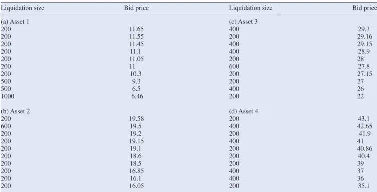
Table 4. Bids of assets 1–4.
Liquidation size Bid price Liquidation size Bid price
(a) Asset 1 (c) Asset 3
200 11.65 400 29.3 200 11.55 200 29.16 200 11.45 400 29.15 200 11.1 400 28.9 200 11.05 200 28 200 11 600 27.8 200 10.3 200 27.15 500 9.3 200 27 500 6.5 400 26 1000 6.46 200 22 (b) Asset 2 (d) Asset 4 200 19.58 200 43.1 600 19.5 400 42.65 200 19.2 200 41.9 200 19.15 400 41 200 19.1 200 40.86 200 18.6 200 40.4 200 18.5 200 39 200 16.85 400 37 200 16.1 400 36 200 16.05 200 35.1 0 0.5 1 1.5 2 2.5 3 x 105 x 105 2.7 2.75 2.8 2.85 2.9 2.95 3 3.05 cash needed portfolio value
Figure 3. Portfolio value with different cash requirements.
4.4. Approximating ladder MSDCs by exponential MSDCs In section 3 we have defined a fast calculation scheme for portfolio valuation with ladder MSDCs. In the real world, however, we may face a situation where to collect the price information to form a ladder MSDC is too costly, or where the information is incomplete or not available, e.g. in an over-the-counter (OTC) market.
As an order book records the trading volume, which forms the basis of MSDCs, one could model ladder MSDCs from the modeling of order book dynamics. For example, Bouchaud
et al.(2002) found that the trading volume at each bid (or ask)
price in the stock order book follows a Gamma distribution.
Contet al.(2010) used a continuous Markov chain to model the evolution of the order book dynamics.
In our paper, we aim to use the basic continuous MSDC mod-els to approximate ladder MSDCs directly, as we can then apply the Lagrange multiplier method and other convex optimization techniques to obtain analytic solutions and thus improve the efficiency.
For actively traded large- or medium-cap security-type as-sets, a portfolio valuation based on exponential MSDCs (20) with their analytic solutions is significantly faster than with ladder MSDCs. For less actively traded small-cap assets, we can use the exponential MSDC model (26) to obtain portfolio values. For OTC-traded assets, lacking price information, the exponential MSDC (28) for small-cap security-type assets with a large liquidity risk factor could be a first modeling attempt.
Generally, when using exponential MSDC models (28) for small-cap security-type assets, we need to estimate or model the parametersmi+andki. The dynamics of the best bidm+i can be read from market data, or modeled by asset price models (e.g., geometric Brownian motion). If we assume that the liq-uidity risk factorkiis independent ofm+i , we can employ time series or stochastic processes to modelki. Ifki is assumed to be correlated withm+i , we also need to model the correlation. Furthermore, for security-type assets traded in an OTC market, we may use the mere price information of the asset to estimate liquidity risk factors in the MSDC models (28). In particular, the liquidity risk factor may be set at a high level to represent the illiquidity of the asset.
For the approximation of ladder MSDCs of illiquid security-type assets using small-cap exponential MSDCs (28), we as-sume that the portfolio consists of only long positions in N
illiquid security-type assets. If we assume that the liquidity risk factor of asseti,ki, is independent of the best bidm+i , then parameterki can be estimated from the ladder MSDC of
Table 5. Liquidity deviation and liquidation sequence.
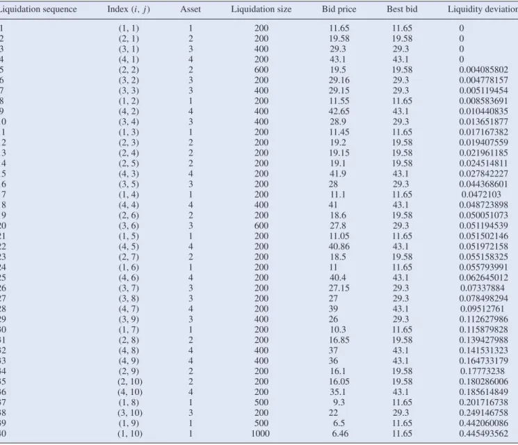
Liquidation sequence Index(i,j) Asset Liquidation size Bid price Best bid Liquidity deviation
1 (1, 1) 1 200 11.65 11.65 0 2 (2, 1) 2 200 19.58 19.58 0 3 (3, 1) 3 400 29.3 29.3 0 4 (4, 1) 4 200 43.1 43.1 0 5 (2, 2) 2 600 19.5 19.58 0.004085802 6 (3, 2) 3 200 29.16 29.3 0.004778157 7 (3, 3) 3 400 29.15 29.3 0.005119454 8 (1, 2) 1 200 11.55 11.65 0.008583691 9 (4, 2) 4 400 42.65 43.1 0.010440835 10 (3, 4) 3 400 28.9 29.3 0.013651877 11 (1, 3) 1 200 11.45 11.65 0.017167382 12 (2, 3) 2 200 19.2 19.58 0.019407559 13 (2, 4) 2 200 19.15 19.58 0.021961185 14 (2, 5) 2 200 19.1 19.58 0.024514811 15 (4, 3) 4 200 41.9 43.1 0.027842227 16 (3, 5) 3 200 28 29.3 0.044368601 17 (1, 4) 1 200 11.1 11.65 0.0472103 18 (4, 4) 4 400 41 43.1 0.048723898 19 (2, 6) 2 200 18.6 19.58 0.050051073 20 (3, 6) 3 600 27.8 29.3 0.051194539 21 (1, 5) 1 200 11.05 11.65 0.051502146 22 (4, 5) 4 200 40.86 43.1 0.051972158 23 (2, 7) 2 200 18.5 19.58 0.055158325 24 (1, 6) 1 200 11 11.65 0.055793991 25 (4, 6) 4 200 40.4 43.1 0.062645012 26 (3, 7) 3 200 27.15 29.3 0.07337884 27 (3, 8) 3 200 27 29.3 0.078498294 28 (4, 7) 4 200 39 43.1 0.09512761 29 (3, 9) 3 400 26 29.3 0.112627986 30 (1, 7) 1 200 10.3 11.65 0.115879828 31 (2, 8) 2 200 16.85 19.58 0.139427988 32 (4, 8) 4 400 37 43.1 0.141531323 33 (4, 9) 4 400 36 43.1 0.164733179 34 (2, 9) 2 200 16.1 19.58 0.17773238 35 (2, 10) 2 200 16.05 19.58 0.180286006 36 (4, 10) 4 200 35.1 43.1 0.185614849 37 (1, 8) 1 500 9.3 11.65 0.201716738 38 (3, 10) 3 200 22 29.3 0.249146758 39 (1, 9) 1 500 6.5 11.65 0.442060086 40 (1, 10) 1 1000 6.46 11.65 0.445493562
assetiby the method of least squares as follows. Provided that
m+i has already been determined, we transform the exponential function as −log(mi(s)/mi+) = s2ki, and estimateki byn discrete pairs(sn,−log(mi(sn)/m+i ))to minimize the merit function: n j=1 −log mi(sj) m+i −s2jki 2 . (32)
The least-squares estimate of parameterkithen reads
ˆ ki = −n j=1s2jlog(mi(sj)/m+i ) n j=1s4j . (33) 5. Numerical results
In this section we give examples for the various concepts discussed in this paper. In particular, we explain the calcu-lation scheme for efficient portfolio valuation by means of an example. Since, for large- or medium-cap security assets, the
uppermost liquidation cost is usually quite small, we will fo-cus on relatively illiquid small-cap security assets and valuate portfolios using ladder MSDCs and exponential MSDCs.
5.1. Portfolio with four illiquid assets
The example here is based on four illiquid small-cap security-type assets. We deal with a portfoliop=(0,3400,2400,3200, 2800) with zero cash asset and long positions in all four illiquid assets. The bid prices with liquidation sizes for the portfolio are chosen at a given time as presented in table4.
It is easy to calculate the uppermost MtM valueU(p)and the liquidation MtM valueL(p)from the table, that isU(p)= 3.01042×10⁵ and L(p) = 2.73720×10⁵. Hence, the up-permost liquidation cost equalsC(p)=0.27322×10⁵. If the true portfolio value is equal to the liquidation MtM value, but, however, if we would use the uppermost MtM value instead, we would overestimate the portfolio value by as much as 10%.
0 500 1000 1500 2000 2500 3000 3500 4 5 6 7 8 9 10 11 12
exp−MSDC vs ladder MSDC for asset A1
s m(s) 0 500 1000 1500 2000 2500 15.5 16 16.5 17 17.5 18 18.5 19 19.5 20
exp−MSDC vs ladder MSDC for asset A2
s m(s) ladder exp 0 500 1000 1500 2000 2500 3000 3500 22 23 24 25 26 27 28 29 30
exp−MSDC vs ladder MSDC for asset A3
s m(s) 0 500 1000 1500 2000 2500 3000 32 34 36 38 40 42 44
exp−MSDC vs ladder MSDC for asset A4
s m(s) ladder exp ladder exp ladder exp
Figure 4. Exponential MSDCs versus ladder MSDCs for the bid prices of assets 1–4.
0 0.5 1 1.5 2 2.5 3 x 105 x 105 2.7 2.75 2.8 2.85 2.9 2.95 3 3.05x 10 5 cash needed portfolio value ladder exp 0 0.5 1 1.5 2 2.5 3 0 0.002 0.004 0.006 0.008 0.01 0.012 0.014 0.016 0.018 0.02 cash needed relative difference
Figure 5. Modeling ladder MSDCs by exponential MSDCs.
For different cash requirements, we use the sorted liquidity deviations (see table5) to find the liquidation sequence and then calculate the portfolio values (see figure3). From the last row of table5, we can see that the liquidity deviation can be as large as 44.5% for the most illiquid part of the MSDC for asset 1, which indicates a high level of liquidity risk.
From figure3, we infer that the portfolio value decreases at a faster rate as we have to liquidate the positions of an increasing number of illiquid assets to meet the cash requirements, which will definitely cause more significant losses during liquidation. The calculation scheme in algorithm1provides an efficient search direction to the optimal value guided by the liquidation sequence. For this four-asset example, we compare our calcu-lation scheme with thefminconfunction with an interior point algorithm in MATLAB for portfolio valuation. The optimiza-tion is repeated for around 2.5×10⁵different cash requirements and the total computation time is recorded.†The averaged time for each cash liquidity policy equals 0.568 milliseconds for our scheme, whereasfmincontakes 202.7 milliseconds, which implies that the time difference is a factor of 300.
Since the ascending sequence of liquidity deviations shows the illiquidity of different parts of the corresponding asset, liquidating a portfolio along the liquidation sequence will cause minimum loss of value compared with the other kinds of liquidation.
5.2. Using exponential MSDCs to approximate ladder MSDCs
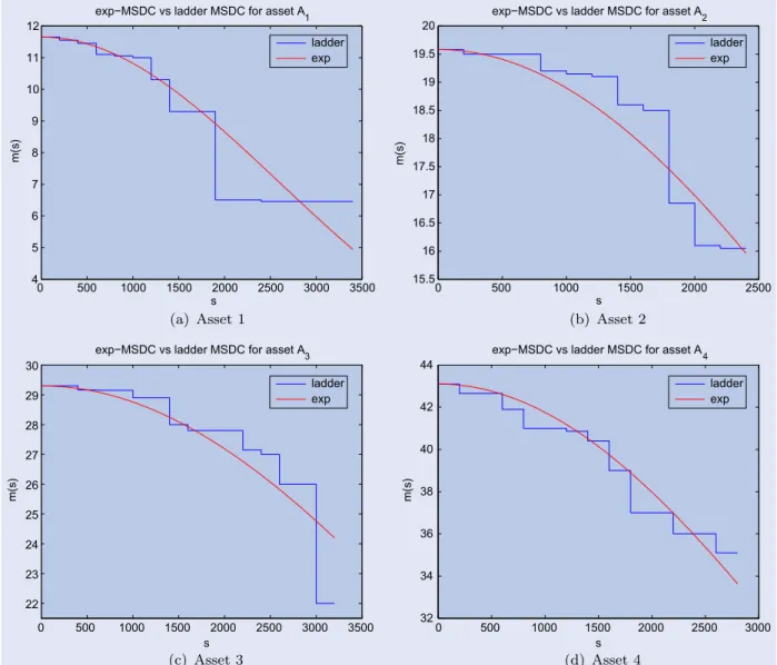
For the four-asset example with the ladder MSDCs from sec-tion 5.1, we use the exponential MSDCs (28) for small-cap equities. Figure4illustrates the ladder MSDCs and the corre-sponding exponential approximating MSDCs. The latter MS-DCs are estimated by least squares (see section4.4).
The liquidity risk factors in the exponential MSDCs are found as k1 = 7.4193×10⁻⁸,k2 = 3.5499×10⁻⁸,k3 = 1.8691×10⁻⁸andk4=3.1634×10⁻⁸. Hence, we infer that asset 1 is the most illiquid and asset 3 is the most liquid, in general.
In figure 5(a), we compare the portfolio values obtained using the exponential MSDCs with the reference portfolio values by the ladder MSDCs under different cash requirements. The relative difference in the portfolio values is presented in figure5(b).
The relative difference found is at most 1.91%, so that, in this example, the exponential MSDCs are accurate approximations. The large approximation error lies in the tail part of the figure and is caused by the illiquidity of the tail parts of assets 1 and 3. This means that the exponential MSDCs may fail to approximate the tail parts of assets 1 and 3 if there are huge drops in price.
6. Conclusion
Within the theory proposed byAcerbi and Scandolo(2008) the valuation of a portfolio can be framed as a convex optimization †The computer used for all experiments has an Intel Core2 Duo CPU, E8600 @3.33 GHz with 3.49 GB of RAM and the code is written in MATLAB R2009b.
problem. We have proposed a useful and efficient algorithm using a specific form of the market data function, i.e. all price information is represented in terms of a ladder MSDC. We have also considered approximations of ladder MSDCs by exponential functions.
As long as the portfolio is valuated using the new models incorporating liquidity risk, one can calculate Value-at-Risk and other risk measures for risk management. Another appli-cation is in portfolio selection. Under the new portfolio theory, the procedure of portfolio selection will become a convex optimization of the allocation based on the convex optimization of portfolio valuation.
By way of future research, methods to estimate the liquidity risk factor in the exponential functions may be improved and more sophisticated models may be considered to replace the exponential functions.
Whereas in regulated markets such as stock exchanges price information is relatively easily available, bid and ask prices for assets traded in the OTC markets may not be readily obtained. Hence, it seems non-trivial to apply this portfolio theory to these types of markets. Extracting all relevant price informa-tion from OTC markets is, however, a challenge.
Acknowledgements
The authors would like to thank Dr Carlo Acerbi (MSCI) for his kind help and fruitful discussions on the theory and the MSDC models. We also thank the anonymous referees for providing us with insightful comments on our first version. The views expressed in this paper do not necessarily reflect the views or practises of RBS.
References
Acerbi, C., Portfolio theory in illiquid markets. InPillar II in the New Basel Accord: The Challenge of Economic Capital,2008 (Risk Books: London).
Acerbi, C. and Finger, C., The value of liquidity: Can it be measured?, 2010 [online]. Available online at: http://www.investmentreview.com/files/2010/07/
The-value-of-liquidity1.pdf(accessed June 2010)
Acerbi, C. and Scandolo, G., Liquidity risk theory and coherent measures of risk.Quant. Finance, 2008,8, 681–692.
Almgren, R., Thum, C., Hauptmann, E. and Li, H., Equity market impact. Risk, 2005, July, 57–62.
Bouchaud, J., Mézard, M. and Potters, M., Statistical properties of stock order books: Empirical results and models.Quant. Finance, 2002,2, 251–256.
Boyd, S. and Vandenberghe, L., Convex Optimization, 2004 (Cambridge University Press: Cambridge).
Cont, R., Kukanov, A. and Stoikov, S., The price impact of order book events, 2011 [online]. Available online at: http://arxiv.org/abs/1011.6402(accessed November 2011) Cont, R., Stoikov, S. and Talreja, R., A stochastic model for order
book dynamics.Oper. Res., 2010,58, 549–563.
Weber, S., Anderson, W., Hamm, A.M., Knispel, T., Liese, M. and Salfeld, T., Liquidity-adjusted risk measures.Math. Financ. Econ., 2013,7, 69–91.