Using Machine Learning to Optimize Parallelism in Big Data Applications
´
Alvaro Brand´on Hern´andeza, Mar´ıa S. Pereza, Smrati Guptab, Victor Munt´es-Mulerob
aOntology Engineering Group, Universidad Politecnica de Madrid, Calle de los Ciruelos, 28660 Boadilla del Monte, Madrid bCA Technologies, Pl. de la Pau, WTC Almeda Park edif. 2 planta 4, 08940 Cornell`a de Llobregat, Barcelona
Abstract
In-memory cluster computing platforms have gained momentum in the last years, due to their ability to analyse big amounts of data in parallel. These platforms are complex and difficult-to-manage environments. In addition, there is a lack of tools to better understand and optimize such platforms that consequently form backbone of big data infrastructure and technologies. This directly leads to underutilization of avail-able resources and application failures in such environment. One of the key aspects that can address this problem is optimization of the task parallelism of application in such environments. In this paper, we propose a machine learning based method that recommends optimal parameters for task parallelization in big data workloads. By monitoring and gathering metrics at system and application level, we are able to find statistical correlations that allow us to characterize and predict the effect of different parallelism set-tings on performance. These predictions are used to recommend an optimal configuration to users before launching their workloads in the cluster, avoiding possible failures, performance degradation and wastage of resources. We evaluate our method with a benchmark of 15 Spark applications on the Grid5000 testbed. We observe up to a 51% gain on performance when using the recommended parallelism settings. The model is also interpretable and can give insights to the user into how different metrics and parameters affect the performance.
Keywords: machine learning, spark, parallelism, big data
1. Introduction
Big data technology and services market is esti-mated to grow at a CAGR1 of 22.6% from 2015 to 2020 and reach $58.9 billion in 2020 [1]. Highly vis-ible early adopters such as Yahoo, eBay and Face-book have demonstrated the value of mining com-plex information sets, and now many companies are eager to unlock the value in their own data. In order to address big data challenges, many different par-allel programming frameworks, like Map Reduce, Apache Spark or Flink have been developed [2, 3, 4]. Planning big data processes effectively on these platforms can become problematic. They involve complex ecosystems where developers need to dis-cover the main causes of performance degradation in terms of time, cost or energy. However, process-ing collected logs and metrics can be a tedious and
Email address: [email protected]( ´Alvaro Brand´on Hern´andez)
1Compound Annual Growth Rate
difficult task. In addition, there are several param-eters that can be adjusted and have an important impact on application performance.
While users have to deal with the challenge of controlling this complex environment, there is a fundamental lack of tools to simplify big data in-frastructure and platform management. Some tools like YARN or Mesos [5, 6] help in decoupling the programming platform from the resource manage-ment. Still, they don’t tackle the problem of opti-mizing application and cluster performance.
One of the most important challenges is finding the best parallelization strategy for a particular ap-plication running on a parallel computing frame-work. Big data platforms like Spark2 or Flink3 use JVM’s distributed along the cluster to perform computations. Parallelization policies can be con-trolled programmatically through APIs or by
tun-2http://spark.apache.org/ (last accessed Jan 2017) 3https://flink.apache.org/ (last accessed Jan 2017)
ing parameters. These policies are normally left as their default values by the users. However, they control the number of tasks running concurrently on each machine, which constitutes the foundation of big data platforms. This factor can affect both correct execution and application execution time. Nonetheless, we lack concrete methods to optimize the parallelism of an application before its execu-tion.
In this paper, we propose a method to recom-mend optimal parallelization settings to users de-pending on the type of application. Our method includes the development of a model that can tune the parameters controlling these settings. We solve this optimization problem through machine learn-ing, based on system and application metrics col-lected from previous executions. This way, we can detect and explain the correlation between an appli-cation, its level of parallelism and the observed per-formance. The model keeps learning from the exe-cutions in the cluster, becoming more accurate and providing several benefits to the user, without any considerable overhead. In addition, we also con-sider executions that failed and provide new config-urations to avoid these kinds of errors. The main two contributions of this paper are:
• A novel method to characterize the effect of parallelism in the performance of big data Workloads. This characterization is further leveraged to optimize in-memory big data ex-ecutions by effective modelling of the per-formance correlation with application, system and parallelism metrics.
• A novel algorithm to optimize parallelism of applications using machine learning. Further-more, a flavour of our proposed algorithm ad-dresses the problem of accurate settings in the execution of applications due to its ability to draw predictions and learn from the compari-son with actual results dynamically.
We choose Spark running on YARN as the frame-work to test our model because of its wide adoption for big data processing. The same principles can be applied to other frameworks, like Flink, since they also parallelize applications in the same manner.
This paper is structured as it follows. Section 2 provides some background about Spark and YARN. In Section 3, we motivate the problem at hand through some examples. Section 4 details the pro-posed model and learning process. In Section 5,
we evaluate the model using Grid 5000 testbed [7]. Section 6 discusses related work. Finally, Section 7 presents future work lines and conclusions.
2. Overview of YARN and Spark 2.1. YARN: A cluster resource manager
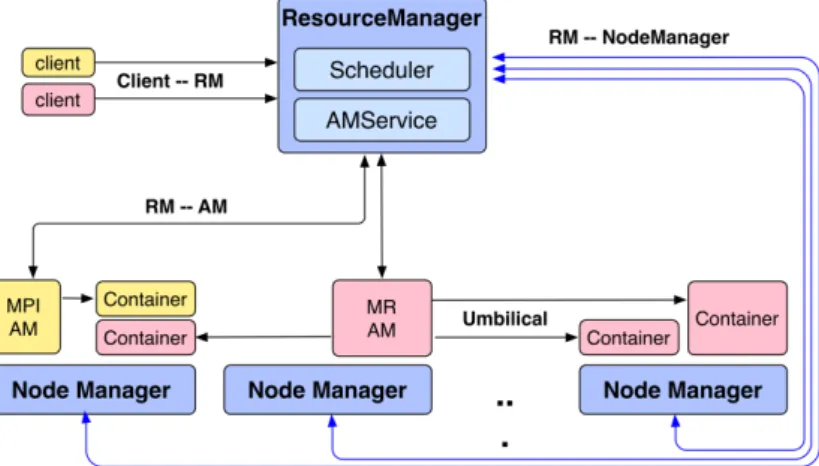
YARN was born from the necessity of decou-pling the programming model from the resource management in the cluster. The execution logic is left to the framework (e.g, Spark) and YARN con-trols the CPU and memory resources in the nodes. This tracking is done through the Resource Man-ager (RM), a daemon that runs in a machine of the cluster.
An application in YARN is coordinated by a unit called the Application Master (AM). AM is respon-sible for allocating resources, taking care of task faults and managing the execution flow. We can consider the AM as the agent that negotiates with the manager to get the resources needed by the ap-plication. In response to this request, resources are allocated for the application in the form of contain-ers in each machine. The last entity involved is the Node Manager (NM). It is responsible for setting up the container’s environment, copying any depen-dencies to the node and evicting any containers if needed. A graphical explanation of the architecture is depicted in Figure 1.
The number of available resources can be seen as a two dimensional space formed by mem-ory and cores that are allocated to containers. Both the MB and cores available in each node are configured through the node manager prop-erties: yarn.nodemanager.resource.memory-mb
andyarn.nodemanager.resource.cpu-vcores re-spectively. An important aspect to take into ac-count is how the scheduler considers these re-sources through the ResourceCalculator. The de-fault option, DefaultResourceCalculator, only con-siders memory when allocating containers while
DominantResourceCalculator, takes into account both dimensions and make decisions based on what is the dominant or bottleneck resource [8]. Since CPU is an elastic resource and we do not want to have a limit on it, we will use the DefaultResource-Calculator for YARN in our experiments. By doing this, we will be able to scale up or down the num-ber of tasks running without reaching a CPU usage limit.
Figure 1: YARN Architecture. In the example a MPI and MapReduce application have their containers running in different nodes. Each node manager is going to have some memory and cores assigned to allocate containers [5]
2.2. Spark: A large data processing engine
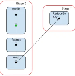
Spark [9] is a fault-tolerant, in-memory data an-alytics engine. Spark is based on a concept called resilient distributed dataset (RDDs). RDDs are immutable resilient distributed collections of data structures partitioned across nodes that can reside in memory or disk. These records of data can be manipulated through transformations (e.g map or filter). A RDD is lazy in the way that will only be computed when an action is invoked (e.g count number of lines, save as a text file). A Spark ap-plication is implemented as a series of actions on these RDDs. When we execute an action over a RDD, a job triggers. Spark then formulates an exe-cution Directed-Acylic-Graph (DAG) whose nodes will represent stages. These stages are composed of a number of tasks that will run in parallel over chunks of our input data, similar to the MapRe-duce platform. In Figure 2 we can see a sample DAG that represents a WordCount application.
When we launch a Spark application, an ap-plication master is created. This AM asks the resource manager, YARN in our case, to start the containers in the different machines of the cluster. These containers are also called executors in the Spark framework. The request consists of number of executors, number of cores per executor and memory per executor. We can provide these values through the --num-executors option together with the parameters spark.executor.cores
and spark.executor.memory. One unit of
spark.executor.cores translates into one task
slot. Spark offers a way of dynamically asking for additional executors in the cluster as long as an application has tasks backlogged and resources available. Also executors can be released by an application if it does not have any running tasks. This feature is called dynamic allocation [10] and it turns into better resource utilization. We use this feature in all of our experiments. This means that we do not have to specify the number of executors for an application as Spark will launch the proper number, based on the available resources. The aim of this paper is to find a combination for spark.executor.memory
and spark.executor.cores to launch an optimal number of parallel tasks in terms of performance.
3. Studying the impact of parallelism
The possibility of splitting data into chunks and processing each part in different machines in a di-vide and conquer manner makes it possible to anal-yse big amounts of data in seconds. In Spark, this parallelism is achieved through tasks that run inside executors across the cluster. Users need to choose the memory size and the number of tasks running inside each executor. By default, Spark considers that each executor size will be of 1GB with one task running inside. This rule of thumb is not opti-mal, since each application is going to have different requirements, leading to wastage of resources, long running times and possible failures in the execution among other problems.
Figure 2: Example DAG for WordCount
We explore these effects in the following exper-iments. We deployed Spark in four nodes of the Taurus cluster in the Grid 5000 testbed [7]. We choose this cluster because we can also evaluate the power consumption through watt-meters in each machine [11]. These machines have two processors Intel Xeon E5-2630 with six cores each, 32GB of memory, 10 Gigabit Ethernet connection and two hard disks of 300 GB. The operating system in-stalled in the nodes is Debian 3.2.68, and the soft-ware versions are Hadoop 2.6.0 and Spark 1.6.2. We configure the Hadoop cluster with four nodes working as datanodes, one of them as master node and the other three as nodemanagers. Each nodem-anager is going to have 28GB of memory available for containers. We set the value of vcores to the same number as physical cores. Note however that we are using all the default settings for YARN and by default the resource calculator is going to be De-faultResourceCalculator [12]. This means that only memory is going to be taken into account when deciding if there are enough resources for a given application. HDFS is used as the parallel filesys-tem where we read the files. We intend to illus-trate the difference in level of parallelism for appli-cations that have varied requirements in terms of I/O, CPU and memory. To this end, we utilize one commonly used application which is CPU intensive, like kMeans and another common one that is inten-sive in consumption of I/O, CPU and memory, like PageRank.
Our objective is to see what is the ef-fect of the number of concurrently running
spark.executor.memory spark.executor.cores 512m 1 1g 1 2g 1 2g 2 2g 3 3g 1 3g 3 3g 4 4g 1 4g 3 4g 6 6g 1
Table 1: Combinations of Spark parameters used for the experiments
tasks on the performance of an application. To do that, we are going to try different combinations of spark.executor.memory and
spark.executor.cores, as seen in Table 1. We choose these values to consider different scenarios including many small JVM’s with one task each, few JVM’s with many tasks or big JVM’s which only host one task.
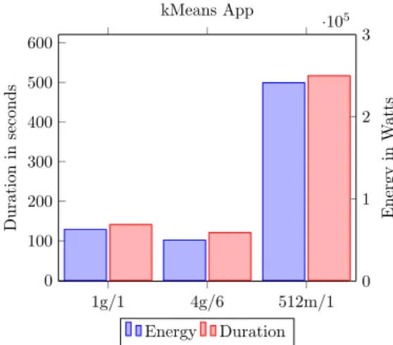
In Figure 3, we can see the time and energy it takes to run a kMeans application in the clus-ter with the default, best and worst configuration. We can observe several effects in both energy and duration for each configuration. Firstly, we ob-serve that the best configuration is 4GB and 6
spark.executor.cores. Since kMeans only shuf-fles a small amount of data, the memory pressure and I/O per task are low, allowing this configura-tion to run a higher number of tasks concurrently and reducing execution times. Additionally, we can see that the worst configuration is the one with 512MB and 1 spark.executor.core. Spark al-lows us to store data in memory for iterative work-loads like kMeans. Sincespark.executor.memory
is sized as 512MB, the system does not have enough space to cache data blocks into the executors. This means that in later stages we will have to read that block from disk, incurring in additional latency, specially if that block is in another rack.
The other example is Page Rank, a graph ap-plication. Its DAG involves many stages and the configuration will have a great impact on the ap-plication performance, as we can see in Figure 4. There is a difference of almost 14 minutes between the best execution and the worst one. In compar-4
1g/1 4g/6 512m/1 0 100 200 300 400 500 600 Duration in seconds kMeans App Energy Duration 0 1 2 3 ·105 Energy in W atts
Figure 3: Run time in seconds and power consumption in watts for a kMeans App. The default, best and worst
configurations are depicted
1g/1 (Failed) 2g/2 6g/1 400 600 800 1,000 1,200 1,400 Duration in seconds
Page Rank App
Energy Duration 0 0.5 1 1.5 2 ·105 Energy in W atts
Figure 4: Run time in seconds and power consumption in watts for a Page Rank App. The default, best and worst
configurations are depicted
ison to kMeans, PageRank caches data into mem-ory that grows with every iteration, filling the heap space often. It also shuffles gigabytes of data that have to be sent through the network and buffered in memory space. The best configuration is the 2g and 2 spark.executor.cores configuration since it provides the best balance between memory space and number of concurrent tasks. For the default one, the executors are not able to meet the mem-ory requirements and the application crashed with an out of memory error. Also, we observed that for the 6g and 1spark.executor.cores, the par-allelism is really poor with only a few tasks running concurrently in each node.
We can draw the conclusion that setting the right
level of parallelism does have an impact on big data applications in terms of time and energy. The de-gree of this impact varies depending on the appli-cation. For PageRank it can prevent the applica-tion from crashing while for kMeans it is only a small gain. Even so, this moderate benefit may have a large impact in organizations that run the same jobs repeatedly. Avoiding bad configurations is equally important. Providing a recommendation to the user can help him to avoid out of memory er-rors, suboptimal running times and wasting cluster resources through constant trial and error runs.
4. Model to find the optimal level of paral-lelism
As we have seen in the previous section, setting the right level of parallelism can be done for each application through its spark.executor.memory
and spark.executor.cores parameters. These
values are supposed to be entered by the user and are then used by the resource manager to allocate JVM’s. However, clusters are often seen as black-boxes where it is difficult for the user to perform this process. Our objective is to propose a model to facilitate this task. Several challenges need to be tackled to achieve this objective:
• The act of setting these parallelization parameters cannot be detached from the status of the cluster: Normally, the user set some parameters without considering the memory and cores available at that moment in the cluster. However, the problem of setting the right executor size is highly dependent on the memory available in each node. We need the current resource status on YARN as a vari-able when making these decisions.
• Expert knowledge about the application behaviour is needed: This needs monitoring the resources consumed and metrics of both the application plus the system side.
• We have to build a model that adapts to the environment we are using: Different machines and technologies give room to differ-ent configurations and parallelism setting. • We have to be able to apply the
experi-ence of previous observations to new ex-ecutions: This will simplify the tuning part to the user every time he launches a new ap-plication.
To solve these problems we leverage the machine learning techniques. Our approach is as follows. First, we will use our knowledge about YARN in-ternals to calculate the number of tasks per node we can concurrently run for different configurations, depending on the available cluster memory. These calculations, together with metrics gathered from previous executions for that application, will form the input of the machine learning module. Then, the predictions will be used to find the best configu-ration. In the following subsections we will explain how we gather the metrics, how we build a dataset that can be used for this problem and the method-ology we use to make the recommendations.
4.1. Gathering the metrics and building new fea-tures
Normally predictive machine learning algorithms need a dataset with a vector of featuresx1, x2, ...xn as an input. In this section we will explain which features we use to characterize Spark applications. They can be classified in three groups:
• Parallelism features: They are metrics that describe the concurrent tasks running on the machine and the cluster. Please note that these are different from the paralleliza-tion parameters. The parallelization pa-rameters are the spark.executor.coresand
spark.executor.memory parameters, which are set up by the users, while the parallelism features describe the effect of these parameters on the applications. We elaborate upon these features in Subsection 4.1.1.
• Application features: These are the metrics that describe the status of execution in Spark. Examples of these features are number of tasks launched, bytes shuffled or the proportion of data that was cached.
• System features: These are the metrics that represent the load of the machines involved. Examples include CPU load, number of I/O operations or context switches.
In the following subsections, we will explain how we monitor these metrics and how we build new additional metrics, like the number of tasks waves spanned by a given configuration or the RDD per-sistence capabilities of Spark. An exhaustive list of metrics is included as an appendix (see Table A.3), together with a notation table, to ease the under-standing of this section (Table B.4).
4.1.1. Parallelism features
A Spark stage spans the number of tasks that are equal to the number of partitions of our RDD. By default, the number of partitions when reading an HDFS file is given by the number of HDFS blocks of that file. It can also be set statically for that imple-mentation through instructions in the Spark API. Since we want to configure the workload parallelism at launch time, depending on variable factors, like the resources available in YARN, we will not con-sider the API approach. The goal is to calculate, before launching an application, the number of ex-ecutors, tasks per executors and tasks per machine that will run with a given configuration and YARN memory available. These metrics will be later used by the model to predict the optimal configuration. To formulate this, we are going to use the calcula-tions followed by YARN to size the containers. We need the following variables:
• Filesize (fsize): The number of tasks spanned by Spark is given by the file size of the input file.
• dfs.block.size (bhdf s): An HDFS parameter that specifies the size of the block in the filesys-tem. We keep the default value of 128MB. • yarn.scheduler.minimum.allocation-mb
(minyarn): The minimum size for any container request. If we make requests under this threshold it will be set to this value. We use its default value of 1024MB.
• spark.executor.memory (memspark): The size of the memory to be used by the executors. This is not the final size of the YARN con-tainer, as we will explain later, since some off-heap memory is needed.
• spark.executor.cores (corspark): The number of tasks that will run inside each executor. • yarn.nodemanager.resource.memory-mb
pa-rameter (memnode): This sets the amount of memory that YARN will have availabe in each node.
• spark.yarn.executor.memoryOverhead
(overyarn): The amount of available off-heap memory. By default, its value its 384.
• Total available nodes (Nnodes): This represents the number of nodes where we can run our ex-ecutors.
The size of an executor is given by:
Sizeexec=memspark+ max(overyarn, memspark∗0.10) (1) The 0.10 is a fixed factor in Spark and it is used to reserve a fraction of memory for the off-heap mem-ory. We then round up the size of the executor to the nearest multiple of yarnminyarn to get the fi-nal size. For example, if we get aSizeexec= 1408, we will round up to two units of minyarn result-ing in Sizeexec = 2048. Now we can calculate the number of executors in each node as Nexec =
bmemnode/Sizeexeccand the number of task slots
in each node as slotsnode = bNexec∗corsparkc. Consequently, the total number of slots in the clus-ter areslotscluster=bslotsnode∗Nnodesc.
Finally, we also want to know the number of waves that will be needed to run all the tasks of that stage. By waves we mean the number of times a tasks slot of an executor will be used, as de-picted in Figure 5. We first calculate the number of tasks that will be needed to process the input data. This is given byNtasks=bfsize/bhdf sc. Then the number of waves is found by dividing this task number between the number of slots in the clus-ter Nwaves = bNtasks/slotsclusterc. Summarizing all the previous metrics that are useful to us, we get the following set of metrics, which we will call parallelism metrics:
{Ntasks, slotsnode, slotscluster, Nwaves, sizeexec, corspark} (2) These are the metrics that will vary depending on the resources available in YARN and the configu-ration we choose for the Spark executors and that will help us to model performance in terms of par-allelism.
4.1.2. Application features
Spark emits an event every time the application performs an action at the task, stage, job and ap-plication levels explained in Section 2.2. These events include metrics that we capture through Slim4, a node.js server that stores these metrics in a
4https://github.com/hammerlab/slim (last accessed Jan
2017)
Figure 5: A set of waves spanned by two executors with three spark.executor.cores. If we have 16 tasks to be executed then it will take three waves to run them in the
cluster
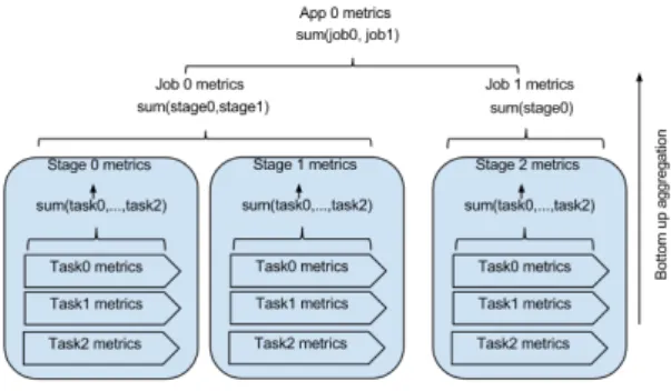
Figure 6: Slim bottom-up aggregation. If we have the metrics for the tasks, Slim can aggregate the ones belonging to a stage to calculate that stage metrics. It does
the same at the job and application execution level
MongoDB5 database and aggregates them at task, stage, job and application level in a bottom to up manner. This means that if we aggregate the coun-ters for all the tasks belonging to a stage, we will have the overall metrics for that stage. The same is done at job level, by aggregating the stage metrics and at application level, by aggregating the jobs, as shown in Figure 6.
This however creates an issue. We want to char-acterize applications, but if we aggregate the met-rics for each tasks then we will have very different results depending on the number of tasks launched. As we explained in Section 4.1.1, the number of tasks spanned depends on the size of the input file. This is not descriptive as we want to be able to de-tect similar applications, based on their behaviour and the operations they perform, even if they op-erate with different file sizes. Let’s assume we have some metrics we gathered by monitoring the only stage of the Grep application with 64 tasks. We need these metrics to describe the application,
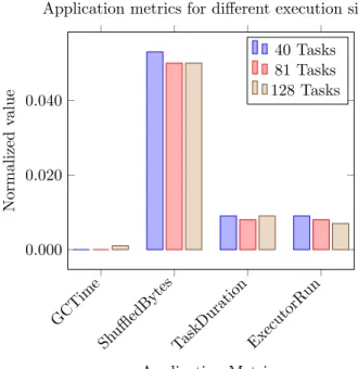
GCTime
ShuffledBytesTaskDuration ExecutorRun 0.000 0.020 0.040 Application Metrics Normalized v alue
Application metrics for different execution sizes 40 Tasks 81 Tasks 128 Tasks
Figure 7: Mean application metrics values for a stage of a Sort application with different filesizes. We can see how the
mean of the metrics is almost the same for 40, 81 and 128 tasks
pendently of the file size with which it was executed. In this example, if this same stage is launched again in the future with 128 tasks, its metrics have to be similar to the ones of the 64 tasks execution in or-der to apply what the model learned so far for Grep or similar behaving applications.
To even out these situations, we calculate the mean of the metrics for the tasks of that stage. Fig-ure 7 shows that the mean gives us similar metrics independently of the filesize for a stage of Sort. The metrics are normalized from 0 to 1 to be able to plot them together, since they have different scales.
We also define an additional metric at the appli-cation level to describe how Spark persists data. We derive a persistence score vector for each stage of an application that describes how much of the total input was read from memory, local disk, HDFS or through the network. For a stageS, we have a to-tal number of task (Ntasks). We count the number of these tasks that read their input from different sources as memory (Nmemory), disk (Ndisk), HDFS (Nhdf s) and networkNnetwork. The vector for that stageVS is: VS = N memory Ntasks , Ndisk Ntasks , Nhdf s Ntasks ,Nnetwork Ntasks
This vector will describe if the stage processes data that is persisted in memory, disk or if it was not on that node at all and had to be read through the network. We also use the HDFS variable to know if the stage reads the data from the dis-tributed file system. Usually this belongs to the first stage of an application, since it is the moment when we first read data and create the RDD.
An important issue to notice here is thatVS can change depending on the execution. Sometimes, Spark will be able to allocate tasks in the same node where the data is persisted. In some other executions, it will not be possible because all slots are occupied or because the system has run out of memory. However, the objective is not to have a de-tailed description of the number of tasks that read persisted data. Instead, we want to know if that stage persists data at all and how much it was able to. Later on, the model will use this to statistically infer how different configurations can affect a stage that persists data.
4.1.3. System features
There are aspects of the workload that cannot be monitored at application level, but at system level, like the time the CPU is waiting for I/O op-erations or the number of bytes of memory paged in and out. To have a complete and detailed sig-nature of the behaviour of an application, we also include these kind of metrics. We include here fea-tures like cpu usr, bytes paged in/out or bytes sent through the network interface. To capture them, we use GMone [13]. GMone is a cloud monitoring tool that can capture metrics of our interest on the different machines of the cluster. GMone is highly customizable and it allows developing plugins that will be used by the monitors in each node. We developed a plugin that uses Dstat6. With this, we obtain a measure per second of the state of the CPU, disk, network and memory of the machines in our cluster.
Since one task will run only in one node, we cal-culate the mean of the system metrics on the node during the lifespan of that task. This will give us descriptive statistics about the impact of that task at the system level. Then, for each stage we will calculate the mean of the metrics for all of its tasks in a similar bottom up way, as we explained Section
6http://dag.wiee.rs/home-made/dstat/ (last accessed
Jan 2017)
in 4.1.2. This will represent what happened at the system level while this application was running.
4.2. Building the dataset and training the model
For each stage executed in our cluster, we get a vector that we use as a data point. We will repre-sent this database of stages as:
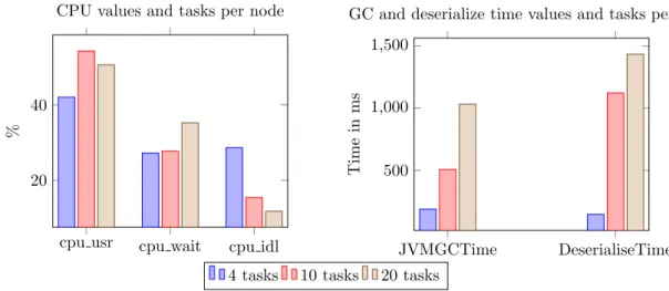
stagesDB={Xapp, Xsystem, Xparallelism, Yduration} where the X’s are the features at application (Sec-tion 4.1.2), system (Sec(Sec-tion 4.1.3) and parallelism level (Section 4.1.1) and Yduration is the duration of that stage or target variable to predict. Now we have to build the dataset that we will use to train the model. We want to answer the following question: If we have a stage with metricsXapp and Xsystem, collected under some Xparallelism condi-tions and its duration wasYduration, what will be the new duration under some differentXparallelism con-ditions?. We can regress this effect from the data points we have from previous executions. However, we have to take into account that metrics change depending on the original conditions in which that stage was executed. For instance it is not the same executing a stage with executors of 1GB and 1 task compared to 3GB and 4 tasks. Metrics like garbage collection time will increase if tasks have less mem-ory for their objects. In addition, CPU wait will increase if we have many tasks in the same machine competing for I/O. We can see this effect in Figure 8, where the metrics of a stage of a support vector machine implementation in Spark change depend-ing on the number of tasks per node we choose.
To solve this variance in the metrics, we have to include two set of parallelism values in the learning process:
• The parallelism conditions under which the metrics were collected. We will call them Xparallelismref.
• The new parallelism conditions under which we will run the application. We will call them Xparallelismrun.
Now building the dataset is just a matter of performing a cartesian product between the met-rics{Xapp, Xsystem, Xparallelism}of a stage and the {Xparallelism, Yduration} of all the executions we have for that same stage. For example, let’s as-sume we have two executions of a stage with differ-ent configurations like 10 and 4 tasks per node. We
also have all their features, including system plus application metrics, and the duration of the stage. The logic behind this cartesian product is: If we have the metrics(X10)and the duration(Y10)of an execution with 10 tasks per node and we have the metrics(X4)and the duration(Y4)of an execution with 4 tasks per node (tpn), then the metrics of the 10 tasks execution together with a configuration of 4 tasks per node can be correlated with the duration of the 4 tpn execution, creating a new point like:
X10app, X10system, X10parallelismref, X4parallelismrun, Y4duration
(3) Note here that we consider that two stages are the same when they belong to the same application and the same position in the DAG. The algorithm is shown in Algorithm 1.
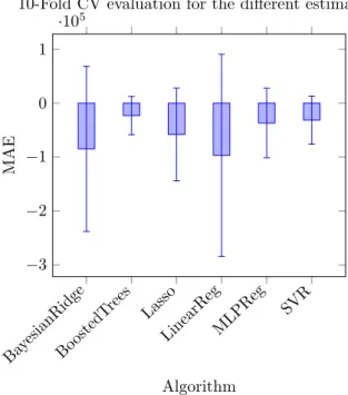
Now we can train the machine learning model with this dataset and check its prediction accuracy. First we have to choose the most accurate imple-mentation. Since this is a regression problem, we try different state-of-the-art regression algorithms: Bayesian Ridge, Linear Regression, SGD Regres-sor, Lasso, Gradient Boosting RegresRegres-sor, Support Vector Regression and MLPRegressor, all from the sklearn Python library [14]. First of all, we choose these regression algorithms versus other solutions, like Deep Learning, because they are interpretable. Apart from this, the chosen algorithms are easily evaluated with cross validation techniques, as K-fold, Leave P-out or Leave One Group Out, among others. From a practical point of view, these al-gorithms are available in the scikit-learn package, which provides implementations ready to be used right out of the box. They also allow us to create pipelines where we perform a series of preprocessing steps before training the model. We build a pipeline for each of the previous algorithms, where we first standardize the data and then fit the model. Stan-dardization of the data is a common previous step of many machine learning estimators. It is performed for each feature, by removing its mean value, and then scaling it by dividing by its standard devi-ation. This ensures an equal impact of different variables on the final outcome and not being biased towards variables that have higher or lower numer-ical values. Then for each pipeline, we perform a ten times cross validation with 3 k-folds [15]. The results are shown in Figure 9. The metric used to evaluate the score is Mean Absolute Error (MAE) [16]. It is calculated by averaging the absolute
er-cpu usr cpu wait cpu idl 20
40
%
CPU values and tasks per node
JVMGCTime DeserialiseTime 500 1,000 1,500 Time in ms
GC and deserialize time values and tasks per node
4 tasks 10 tasks 20 tasks
Figure 8: Changes in the metrics for a stage of a support vector machine implementation in Spark. Note how the CPU metrics change depending on the number of tasks per node. Also garbage collection and the deserialize time of an stage
increases with this number
Algorithm 1Building the training dataset for the machine learning algorithm
1: procedurebuildataset
2: stages={(Xapp, Xsystem, Xparallelism, Yduration)n} . The stage executions that we have
3: dataset=∅
4: for alls∈stagesdo
5: B={x∈stages|x=s} .All the stages that are the same as s
6: new=s[Xapp, Xsystem, Xparallelismref]×B[Xparallelismrun, Yduration]
7: addnewto dataset
8: end for 9: returndataset
10: end procedure
rors between predicted and true values for all the data points. MAE will allow us to evaluate how close the different predictors are to the real values. We do not include SGD Regressor, since its MAE is just too high to compare with the other meth-ods. As we can see, boosted regression trees have the best accuracy amongst the seven methods and also the lowest variance. In addition, decision trees are interpretable. This means that we will be able to quantify the effect of any of the features of the model on the overall performance of the applica-tion.
4.3. Using the model: providing recommendations for applications
So far, we have only characterized and built our model for stages. An application is a DAG made out of stages. So how we provide a paralleliza-tion recommendaparalleliza-tion based on the previous ex-plained concepts?. Remember that a configuration in Spark is given at application level. Thus, if we set some values for spark.executor.memory and
spark.executor.cores, they will be applied to all the stages. If we have a listlistof conf swith com-binations of different values for these two parame-ters, and we launch an application with a different combination each time, each execution will have dif-ferent tasks per node, waves of tasks and memory per task settings. In other words, and following the previously introduced notation, each execution will have different Xparallelism features. The dataset built in Algorithm 1 had data points like:
{Xapp, Xsystem, Xparallelismref, Xparallelismrun, Yduration} (4) therefore, we can plug in new values for Xparallelismrun by iterating through the different configurations inlistof conf s, and predict the new Yduration for the parameters. In addition, the ob-jective is to know the effect of a given configuration on the whole application. So we can perform this process for all the stages that are part of the ap-plication and sum the predictions for each config-uration. Then we only have to choose as the opti-mal configuration the one from the list that yields the minimum predicted duration. Algorithm 2 de-scribes this process for a given application and its input data size. The time complexity of the boosted decision trees model, used to make the predictions,
isO(ntree∗n∗d), wherentreeis the number of trees
of the boosted model,dis the depth of those trees andnis the number of data points to be predicted.
Baye sianRid ge BoostedT rees Lasso LinearRegMLPReg SVR −3 −2 −1 0 1 ·105 Algorithm MAE
10-Fold CV evaluation for the different estimators
Figure 9: 10 CV with 3 K-Fold MAE score for different regression algorithms. GradientBoostingRegressor is the clear winner with a median absolute error of 23 seconds, a
maximum of 94 seconds in the last 10th iteration and a minimum of 2.7 seconds for the 3rd iteration
We have to do this prediction for thenconf configu-rations of the configuration list, which transforms it
intoO(ntree∗n∗d∗nconf). Note that the only term
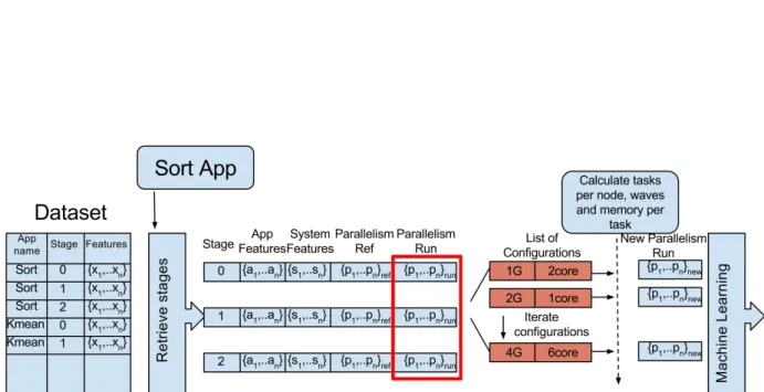
that is variable here is the number of data pointsn, that will grow as we have more executions on our system. The rest will remain constant as they are fixed the moment we train the model and are small numbers. We have to point out that we do not con-sider stages that launch only one task, since it is trivial that parallelism will not bring any benefit to them. The DAG engine of Spark can also detect that some stages do not have to be recomputed and so they can be skipped. We do not consider these kind of stages in the DAG either since their runtime is always 0. Figure 10 shows a graphical depiction of the workflow for a Sort app example.
4.4. Dealing with applications that fail
When we explained the process by which we pre-dict the best parallelism configuration, we assumed that we have seen at least once all the stages of an application. However, this is not always the case, since some configurations may crash. For exam-ple, for a Spark ConnectedComponent application with a filesize of 8GB, the only configurations that
Algorithm 2Recommending a parallelism configuration for an application and its input datasize
1: procedurepredictconfboosted(app, f ilesize, listof conf s)
2: S={s∈stages|s∈DAG(app)} . All the stages that belong to the app
3: listof conf sandduration=∅
4: for allconf ∈listof conf sdo 5: for alls∈S do
6: if s.ntasks6= 1then . Some stages only have on task. We do not consider those
7: s[Xparallelismrun] =calculateP arallelism(f ilesize, conf) .As explained in 4.1.1
8: duration=duration+predictBoostedT rees(s) . we accumulate the prediction of each
stage
9: end if
10: end for
11: add(duration, conf)to listof conf sandduration
12: end for
13: returnmin(listof conf sandduration)
14: end procedure
Figure 10: An example with a Sort App, where we iterate through a configuration list. Notice the different parallelism features: {p1, ..., pn}ref represent the parallelism conditions under which the metrics were collected,{p1, ..., pn}runthe
parallelism conditions under which the application run for that execution and{p1, ..., pn}new the new parallelism conditions
that we want to try and the ones we will pass to the machine learning module. The rest of the metrics are kept constant. Then we just have to group by configuration and sum up each of the stages predictions to know which one is best
Figure 11: A deadlock situation in which the same configuration is recommended continuously. The application crashes with the default configuration. Based
on whichever stages executed successfully the next recommendation also crashes. If we do not get past the crashing point the recommendation will always be the same
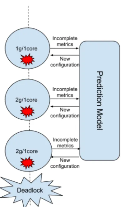
were able to complete successfully in our experi-ments were the ones with 4GB and 1 core and 6GB and 1 core. The reason behind it is that graph processing applications are resource hungry and it-erative by nature. This can put a lot of pressure in the memory management, specially when we cache RDD’s like in these kind of implementations. In this particular example, the 8GB file we initially read from HDFS grows to a 17.4GB cached RDD in the final stages of the application.
Thus, if we choose an insufficient memory setting, like the default 1GB configuration, the application will not finish successfully and we will not have ei-ther the complete number of stages or the metrics for that application. Incomplete information means that the next configuration recommended could be non-optimal, drawing us into a loop where the ap-plication continuously crashes, as depicted in Fig-ure 11.
To solve this, we use the approach explained in Algorithm 3. When a user launches an applica-tion, we check if there are any successful executions for it. If we cannot find any then we retrieve the furthest stage the application got to. This can be considered as the point where the execution could
not continue. For that stage we find the k-nearest neighbours from all the stages that we have seen so far. These neighbouring stages belong to a set of applications. Then we follow a conservative ap-proach where we choose the configuration amongst these applications that resulted in the most num-ber of stages completed. The intuition behind it is that a configuration with a high number of com-pleted stages means better stability to the appli-cation. With this, we aim to achieve a complete execution of the application and to collect the fea-tures of all the stages with it. If the user executes the same application in the future, we can use this complete information together with the standard boosted gradient model to recommend a new config-uration. By trying different values for the number of k neighbours, we found that 3 is a good number for this parameter. Going above this value can re-trieve too many diverse stages, which could make the application to crash again. Going below it can take us to the same deadlock depicted in Figure 11. Remember that the objective is not to find an optimal configuration, but a conservative configu-ration, which enables a complete execution without failures.
The kNeighbours approach uses a K-D Tree search approach, where the complexity isO(log(n)) withnbeing the number of data points.
4.5. The recommendation workflow
Now that we have developed the models with which we make recommendations, we can connect everything together and describe the workflow we follow to find the best parallelism settings. When a user wants to execute an application, first we check if we have any information of it in our database of previously seen applications. If we do not have it, we execute it with the default configuration. This execution will give us the metrics we need to tune the application in future executions. If we do have information about that application, we check if it completed successfully or not:
• In case it did not, we apply the procedure of Algorithm 3 for crashed executions.
• In case it did, we apply the Algorithm 2 with the boosted regression trees model.
Whatever the case is, the monitoring system adds the metrics for that run to our database so they can be applied for future executions. Applications in a cluster are recurring [17]. This means that the
Algorithm 3Finding a configuration for an application that failed
1: procedurepredictconfkneighbours(app)
2: S={s∈stages|s∈DAG(app)∧s[status] =f ailed}
3: x=lastexecutedstage∈S
4: neighbours=f ind3neighbours(x, stages)
5: res={n∈neighbours|n.stagesCompleted=max(n.stagesCompleted)}
6: returnres.conf iguration
7: end procedure
precision of the model will increase with the time since we will have more data points. We assume the machine learning algorithm has been trained beforehand and we consider out of the scope of this paper and as future work, when and how to retrain it. A final algorithm for the process is depicted in Algorithm 4.
5. Evaluation
We perform an offline evaluation of the model with the traces we got from a series of experiments in Grid 5000.
Cluster setup: Six nodes of the Adonis clus-ter in the Grid 5000 testbed. These machines have two processors Intel Xeon E5520 with four cores each, 24GB of memory, 1 Gigabit Ethernet and 1 card InfiniBand 40G and a single SATA hard disk of 250 GB. The operating system installed in the nodes is Debian 3.2.68, and the software ver-sions are Hadoop 2.6.0 and Spark 1.6.2. We con-figure the Hadoop cluster with six nodes working as datanodes, one of them as master node and the other five as nodemanagers. Each nodemanager has 21GB of memory available for containers. We set the value of vcores to the same number as physical cores. We build a benchmark that is a combination of Spark-bench [18], Bigdatabench [19] and some workloads that we implemented on our own. The latter ones were implemented to have a broader va-riety of stages and each one has different nature:
• RDDRelation: Here we use Spark SQL and the dataframes API. We read a file that has pairs of (key, value). First we count the number of keys using the RDD API and then using the Dataframe API with aselect count(*)type of query. After that, we do a select from
query in a range of values and store the data in a Parquet data format7. This workflow consist
7https://parquet.apache.org/ (last accessed Jan 2017)
of four stages in total.
• NGramsExample: We read a text file and we construct a dataframe where a row is a line in the text. Then we separate these lines in words and we calculate the NGrams=2 for each line. Finally these Ngrams are saved in a text file in HDFS. This gives us a stage in total since it is all a matter of mapping the values and there is no shuffles involved.
• GroupByTest: Here we do not read any data from disk but we rather generate an RDD with pairs of (randomkey, values). The keys are generated inside a fixed range so there will be duplicate keys. The idea is to group by key and then perform a count of each key. The number of pairs, the number of partitions of the RDD and consequently the number of tasks can be changed through the input parameters of the application. This gives us two stages like in a typical GroupBy operation.
We run all the applications of this unified bench-mark with three different file sizes as we want to check how the model reacts when executing the same application with different amounts of data. Some implementations, like the machine learning ones, expect a series of hyperparameters. These are kept constant across executions and their effect is left out of the scope of this paper. We also try different values for spark.executor.memory and
spark.executor.cores for each application and data size combinations. These executions generate a series of traces that we use to train and evaluate our model offline. Since the usefulness of our ap-proach is that it can predict the performance of new unseen applications, we train the model by leav-ing some apps outside of the trainleav-ing set. Those apps will be later used as a test set. A descrip-tion of the benchmark is depicted in Table 2. The reason for choosing this benchmark, is to have a 14
Algorithm 4Providing an optimal configuration for a application and a given input file size
1: procedureconfigurationforapplication(application, f ilesize)
2: A={apps∈appDB|apps.name=application)}
3: if A=∅ then 4: conf = (1g,1)
5: else if A6=∅then
6: if (∀app∈A|app.status=f ailed) then
7: conf =predictconf kneighbours(app)
8: else
9: conf =predictconf boosted(app, f ilesize)
10: end if 11: end if
12: submittospark(app, conf)
13: addmonitored features tostageDBandappDB 14: end procedure
representative collection of batch processing appli-cations that are affected differently by their paral-lelization, i.e. graph processing, text processing and machine learning. These three groups allow us to prove that applications with different resource con-sumption profiles have different optimal configura-tions. We leave as future work the effect of paral-lelization in data streaming applications. The files were generated synthetically. At the end we have 5583 stages to work with. As before we use the dynamic allocation feature of Spark and the De-faulResourceAllocator for YARN.
5.1. Overhead of the system
In this section, we want to evaluate the overhead of monitoring the system, training the model and calculating a prediction. The first concern is if Slim and GMone introduce some overhead when launch-ing applications. We executed five batches of two applications running in succession: Grep and Lin-earRegression. We measured the time it took to execute these five batches with and without moni-toring the applications. The results are depicted in Figure 12. As we can see, the overhead is negligible. Also we want to evaluate how much time it takes to train the model and to calculate the optimal con-figuration for an application. We train the model with the traces we got from Grid5000 in our local computer. The specifications for the CPU are 2,5 GHz Intel Core i7 of 4 cores and for the memory is 16GB of DDR3 RAM. The overhead of training the model depends on the number of data points, as shown in Figure 13. For the complete training set of 55139 the latency is 877 seconds. For the overhead
Monitored Non-monitored 0.00 20.00 40.00 60.00 80.00 100.00 120.00 Duration in seconds
Overhead of the monitoring system
Figure 12: Overhead introduced by monitoring and storing the traces versus non-monitoring. As we can see the
Table 2: Different applications used. File size denotes the three different sizes used for that application. Group by doesn’t read any file but creates all the data directly in memory with 100 partitions
Application Dataset Split File Size Type of App
ShortestPath Test 20GB,11GB,8GB Graph Processing Connected Component Logistic Regression 18GB,10GB,5GB Machine Learning Support Vector Machine
Spark PCA Example
Grep Text Processing
SVDPlusPlus
Train
20GB,11GB,8GB Graph Processing Page Rank
Triangle Count
Strongly Connected Component Linear Regression 18GB,10GB,5GB Machine Learning kMeans Decision Tree Tokenizer Text Processing Sort WordCount RDDRelation SparkSQL
GroupBy 100 tasks Shuffle
of the predictions, we take all the data points in the test set for each application and predict their execution times. As we can see in Figure 14, the overhead is negligible, with a maximum latency of 0.551 seconds for the LogisticRegression App that has 10206 points in the test set. Note that this pro-cess is run on a laptop but it can be run on a node of the cluster with less load and more computation power, like the master node. We must also consider that we trained the model with sklearn, but there are distributed implementations of boosted regres-sion trees in MLlib8for Spark that can speed up the process. We leave as future work when and how the model should be trained.
5.2. Accuracy of predicted times
Now we evaluate the accuracy of the predicted durations. As we mentioned earlier, we built the training and the test set by splitting the benchmark in two different groups. First, we start by evaluat-ing the duration predictions for different stages. To do that, we take all the data points for a stage, we feed them to the model and we average the pre-dictions for each configuration. The results can be seen in Figure 15. For some stages, the predictions are really precise, like the stage 0 of Shortest Path
8http://spark.apache.org/mllib/ (last accessed Jan 2017)
20,000 40,000 60,000 80,000 0
500 1,000 1,500
Number of data points
Duration
in
seconds
Overhead of training the model
Figure 13: Duration of training the model depending on the number of data points. For the whole dataset of 85664
points the duration is 1536 seconds.
PCA Grep SVM ShortestP ath LogisticReg ConComp onen t 0.00 0.20 0.40 0.60 Duration in seconds
Overhead of the predictions
Figure 14: Latency in the predictions for different applications. The latency is always less than 1 second with
a maximum of 0.519 for a Logistic Regression App
with 8GB. Some others, like the Stage 1 of Support Vector Machine for 10GB, do not follow the ex-act same trend as the real duration but effectively detect the minimum. We show here some of the longest running stages across applications, since op-timizing their performance will have a greater im-pact on the overall execution. Remember that our final objective is not to predict the exact run time but rather to know which configurations will affect negatively or positively the performance of an ap-plication.
5.3. Accuracy of parallelism recommendations for an application
Now that we have seen the predictions for sep-arate stages, we are going to evaluate the method for a complete application. The objective is to com-pare our recommendations with a default configu-ration that a user will normally use and with the best improvement the application can get. We also want to evaluate how the predictions evolve with time, as we add more data points to our database of executions. To achieve that, we are going to as-sume a scenario where the user launches a set of applications recurrently with different file sizes. If the application has not been launched before, the recommendation will be the default one. After that
first execution, the system will have monitored met-rics for that application. We can start recommend-ing configurations and the user will always choose to launch the workload with that configuration. In the scenario, for the non-graph applications in the test set, the user executes each one with 5GB, 10GB and 18GB consecutively. For the graph applications we do the same with their 20GB, 8GB and 11GB sizes. In this case, we invert the order, since none of the 20GB executions finished correctly because of out of memory errors and we use them to get the metrics instead. The results of these executions can be seen in Figures 16 and 17. Note how we separate the figures for graphs and non-graph ap-plications. The reason is that with one gigabyte for spark.executor.memory, the graph workloads always crashed, so we do not include this default execution. Best shows the lowest possible latency that we could get for that application. Predicted is the configuration proposed by our model. Default
is the runtime for a 1g/1core configuration. Worst
is the highest run time amongst the executions that finished successfully. We do not show here any ap-plication that did not complete successfully. For some applications the recommendations achieve the maximum efficiency like Grep with 10GB, Logistic Regression with 18GB or SVM with 18GB. For ex-ample in Grep 10GB the maximum improvement is of 11%. This means 11% of savings in energy and resource utilization, which may be significant when these applications are executed recurrently. These recommendations can also help the user to avoid really inefficient configurations, like the one in Grep 10GB. For graph executions, the benefits are more obvious. Since the initial default execu-tion always crashed, the first recommendaexecu-tion by the system was drawn out of the neighbours proce-dure explained early. The latency for this first rec-ommendation is not optimal, but we have to keep in mind that this is a conservative approach to get a first complete run and a series of traces for the application. After getting this information and ap-plying the boosted model, we can get an improve-ment up to 50% for the case of connected compo-nent with 11GB. We also want to prove that the model can converge to a better solution with ev-ery new execution it monitors. Note that we are not talking about retraining the model, but about using additional monitored executions to improve the accuracy. As an example, we keep executing the shortest path application first with 11GB and then with 8GB until the model converges to an
op-1g 1 2g 1 2g 2 2g 3 3g 1 3g 4 4g 1 4g 3 6g 1 100 200 300 400 Time in seconds
Stage 0 of 8GB Shortest Path
1g 1 2g 1 2g 2 2g 3 3g 1 3g 4 4g 1 4g 3 6g 1 60 80 100 Stage 1 of 10GB SVM 1g 1 2g 1 2g 2 2g 3 3g 1 3g 4 4g 1 4g 3 6g 1 90 100 110
Stage 1 of 18GB Logistic Regression
Real duration Predicted duration
Figure 15: Predictions for stages of different apps with the highest duration and so highest impact inside their applications. For Shortest Path the predictions are pretty accurate. For SVM and Logistic Regression the trend of the predicted values
follows the real ones.
timal solution. The evolution can be seen in Figure 18. For the 11GB execution, the first point is the duration for the neighbours approach. After that, the execution recommended with the boosted re-gression model fails, but the model goes back to an optimal prediction in the next iteration. In the 8GB case, it goes down again from the conserva-tive first recommendation to a nearly optimal one. This is an added value of the model. The system can become more intelligent with every new execu-tion and will help the user to make better decisions about parallelism settings.
Finally, we include in Figure 19 the time that it takes to find an optimal configuration for each application. For the boosted decision trees ap-proach, the average overhead is 0.3 seconds and it increases slightly for those applications that have more stages, like logistic regression. We consider this negligible, since a 0.3 seconds delay will not be noticeable by the user. The kNeighbours approach is faster, but it is only applied to those applications that crash with the default execution of 1g/1core.
5.4. Interpretability of the model
Another advantage of decision trees is that they are interpretable. That means that we can evaluate the impact of certain features on the outcome vari-able (duration in our case). One of the possible ap-plications is to explain how the number of tasks per node affects a given workload. This information can be valuable when the user wants to manually choose a configuration. For example, in Figure 20 we see the partial dependence of three applications. Short-est Paths is a graph processing application and, as
we saw earlier, it benefits from a low number of tasks per node. KMeans sweet spot seems to be around a default 10-12 tasks per node. For PCA, the points between 0 and 5 correspond to stages with only one or few tasks, something very common in machine learning implementations. Again every-thing from 8 to 15 is a good configuration while more than that, it is counterproductive. Also note how the partial dependence shows us the degree to which parallelism affects that workload. For exam-ple in Shortest Paths it ranges from 2000 to -4000 while in kMeans it goes from 100 to -100. Indeed, as we saw in the experiments of the motivation sec-tion, the benefit of parallelism is more obvious on graph applications than in kMeans. This feature of a decision tree proves to be useful and can help the user to understand how different parameters affect their workloads.
6. Related Work
There are several areas of research that are re-lated to our work:
Using historical data to predict the out-come of an application: Several lines of research try to optimize different aspects of applications. In [20], the authors present the Active Harmony tun-ing system. It was born from the necessity to auto-matically tune scientific workflows and e-commerce applications. The challenge lies on choosing an op-timal parametrization from a large search space. To narrow this space, it considers only the parameters that affect performance the most. In contrast, we 18
PCA 18GB PCA 10GB Grep 18GB Grep 10GB SVM 18GB SVM 10GB LogRegr 18GB LogRegr 10GB 100 200 Time in seconds Non-graph executions Best Predicted Default Worst
Figure 16: Executions for the non-graph processing applications of the test set. Best shows the lowest possible latency that we could get for that application. Predicted is the configuration proposed by our model. Default is the runtime for a 1g and 1
task slot per executor configuration. Worst is the highest run time amongst the executions that finished successfully
ShortP ath 8GB ShortP ath 11GB ConComp onen t8GB ConComp onen t11GB 0 10,000 20,000 Time in seconds Graph executions
Best Predicted Worst
Figure 17: Executions for the graph processing applications of the test set. Best shows the lowest possible latency that
we could get for that application. Predicted is the configuration proposed by our model. Worst is the worst
running time. All the default configurations crashed for these kinds of applications
kNeigh bours 1st boosted 2nd boosted 3rd boosted 1,000 2,000 3,000 11GB Optimal 8GB Optimal Error Time in seconds
Evolution of Shortest Path 8GB 11GB
Figure 18: Evolution for the predictions of a recurrently executed shortest path application. From the conservative
kNeighbours approach, we go to nearly optimal execution times. Note how the first prediction of the boosted model
PCA Grep SVM ShortestP ath LogisticReg ConComp onen t 0.000 0.100 0.200 0.300 0.400 0.500 Duration in seconds
Time to calculate recommended configuration BoostedTrees
kNeighbours
Figure 19: Time needed to calculate a recommended configuration with the boosted regression method and the
kNeighbours method for each of the applications in our simulated scenario. Note that some of the applications do
not use the kNeighbours method, since it is needed only when the application crashes with the default configuration
of 1g and 1 core
do not need to narrow the parameter space, be-cause we evaluate the performance of a configura-tion through the machine learning module, which has a negligible overhead. Another different ap-proach in [21] is to use a benchmark of HPC work-loads from different domains to create a reference database of execution profiles. These profiles are called kernels. The paper presents a framework with the reference kernel implementations, their ex-ecution profiles and a performance model already trained that can predict their execution time with other problem sizes and processor. Our solution does not need this reference database already built and it dynamically creates the model with every new execution that comes in. There is work that considers the characteristics of the input data as an input to the learning model. In [22], the authors sample from the data a series of characteristics (e.g number of numerical and categorical attributes of the dataset) that constitute the variables of a lin-ear regression model that predicts the run time of a C4.5 algorithm. However, they do not consider how we can speed up applications or any configuration parameters. Multilayer neural networks were used
in [23] to predict execution times on the parallel ap-plication SMG2000. It explains a typical machine learning process where data from different execu-tions is gathered into a training and a test set. A problem of neural networks though is that they are not interpretable. This does not suit our objective of assisting the user when using big data platforms.
Optimizing and predicting performance of Hadoop: When Hadoop was the main tool for big data analytics, a series of publications focused on optimizing its default settings. Starfish [24] is an auto-tuning system for MapReduce that optimizes the parametrization through a cost based model. However, this model introduces a profiling overhead and is rigid, meaning that if the underlying infras-tructure changes, so should the model. A machine learning approach can adapt itself by training on new data. The authors in [25] propose a method to predict the runtime of Jaql queries. It trains two models for each query type: one to predict the processing speed of the query and a second one to predict the output cardinality. A query is consid-ered similar to another one if they have the same jaql functions. With these two models we can esti-mate the execution time. This is a really restrictive model, especially to new incoming queries that does not have any other similar observations. Our model does not need any features of a specific domain like jaql but relies instead on more general Spark and machine metrics. It can also be applied to any new incoming observations. ALOJA-ML [26] uses ma-chine learning techniques to tune the performance of Hadoop and discover knowledge inside a repos-itory of around 16.000 workload executions. This allows the authors to evaluate the impact of vari-ables like hardware configurations, parameters and cloud providers. However, Spark works in a dif-ferent way compared to Hadoop, specially because of its in-memory computing capabilities. In [27], the authors also study how to configure a MapRe-duce job in addition to calculating the number of virtual machines and its size needed to run that application. It does so by clustering applications that show a similar CPU, memory and disk usage rate. For each cluster, it builds a SVM regression model. In contrast, our approach does not need to cluster similar applications together but generalizes depending on the features of the workload. MROn-line [28] provides an onMROn-line tuning system that is based on statistics of the job and a gray-box smart hill climbing algorithm. The tuning is made at task level. This system is oriented to MapReduce and 20
0 10 20 −4,000
−2,000 0 2,000
Tasks per Node
P artial De p endence Shortest Paths 10 20 −100 0 100
Tasks per Node
P artial De p endence kMeans 0 10 20 −500 0 500
Tasks per Node
P
artial
Dep
endence
PCA
Figure 20: Partial dependence for different applications. Shortest Paths works better with a low number of tasks per node. kMeans best setting is 12 tasks per node. For PCA the points between 0 and 5 corresponds to stages with only one or few
tasks, while with many tasks 7 is a good configuration
needs tasks test runs to converge into the optimal solution. Cheng et al. [29] use genetic algorithms to configure MapReduce tasks in each node, taking into account cluster heterogeneity. The parameters are changed, depending on how well a parameter value works in a machine. However, it does not work well for short jobs, since it needs time to con-verge into a good solution.
Optimizing and predicting performance of Spark: Spark is a relatively new technology and its popularity is on the rise. Tuning up its perfor-mance is an important concern of the community and yet there is not much related work. In [30], the authors present, to the best of our knowledge, the only Apache Spark prediction model. Again sampling the application with a smaller data size is used to get statistics about the duration of the tasks and plugged into a formula that gives an esti-mation of the total run time for a different file size. However, it does not considers tuning any parame-ters and their effect on duration. MEMTune [31] is able to determine the memory of Spark’s executors by changing dynamically the size of both the JVM and the RDD cache. It also prefetchs data that is going to be used in future stages and evicts data blocks that are not going to be used. However, the method is an iterative process that takes some time to achieve the best result and it does not work well with small jobs. It does not learn from previous executions either. In [32], the authors perform sev-eral runs of a benchmark and iterate through the different parameters of Spark to determine which ones are of most importance. With the experience acquired from these executions, they build a block diagram through a trial and error approach of
dif-ferent parameters. The obvious drawback is that we have to execute the application several times and follow the process every time the input size changes. Tuning garbage collection has also been considered in [33]. The authors analyse in depth the logs of JVM usage and come to the conclusion that G1GC implementation improves execution times. Finally, in [34], a new model for shuffling data across nodes is proposed. The old model of creating a file in each map tasks for each reduce task was too expensive in terms of IO. Their solution is to make the map tasks running in the same core write to the same set of files for each reduce task.
Task contention: One of the objectives of our model is to detect task contention and act accord-ingly, by increasing or decreasing the number of tasks. This topic has also been explored in [35]. Bubble up proposes a methodology to evaluate the pressure that a given workload generates in the sys-tem and the pressure that this same workload can tolerate. With this characterization, better colo-cation of tasks can be achieved. Nonetheless, this requires using the stress benchmark in all the new applications that we launch. Paragon [36] takes into account both heterogeneity of machines and contention between tasks when scheduling. By us-ing SVD, it can calculate performance scores of a task executed in a given machine configuration and co-located with another workload. Same as in pre-vious references, it needs benchmarking each time a different workload comes in. Moreover, we are not trying to create a scheduler, but to assist the user in using big data platforms. In [37], the au-thors propose another scheduler that is based on the assumption that resource demands of the