Detection of chronic kidney disease using machine learning algorithms with least number of predictors

Detection of Chronic Kidney Disease Using Machine

Learning Algorithms with Least Number of Predictors

Marwa Almasoud

Riyadh, Saudi Arabia Email: [email protected]

Tomas E Ward

Insight Center for Data Analytics Dublin City University

Dublin, Ireland Email: [email protected]

Abstract— Chronic kidney disease (CKD) is one of the most

critical health problems due to its increasing prevalence. In this paper, we aim to test the ability of machine learning algorithms for the prediction of chronic kidney disease using the smallest subset of features. Several statistical tests have been done to remove redundant features such as the ANOVA test, the Pearson’s correlation, and the Cramer’s V test. Logistic regression, support vector machines, random forest, and gradient boosting algorithms have been trained and tested using 10-fold cross-validation. We achieve an accuracy of 99.1 according to F1-measure from Gradient Boosting classifier. Also, we found that hemoglobin has higher importance for both random forest and Gradient boosting in detecting CKD. Finally, our results are among the highest compared to previous studies but with less number of features reached so far. Hence, we can detect CKD at only $26.65 by performing three simple tests.

Keywords— chronic kidney disease (CKD), Random forest (RF), Gradient boosting (GB), Logistic Regression (LR), Support vector machines (SVM), Machine learning (ML), prediction.

I. INTRODUCTION

Chronic kidney disease (CKD) is a significant public health problem worldwide, especially for low and medium-income countries. Chronic kidney disease (CKD) means that the kidney does not work as expected and cannot correctly filter blood. About 10% of the population worldwide suffers from (CKD), and millions die each year because they cannot get affordable treatment, with the number increasing in the elderly. According to the Global Burden Disease 2010 study conducted by the International Society of Nephrology, chronic kidney disease (CKD) has been raised as an important cause of mortality worldwide with the number of deaths increasing by 82.3% in the last two decades [1, 2]. Also, the number of patients reaching end-stage renal disease (ESRD) is increasing, which requires kidney transplantation or dialysis to save patients' lives [1, 3, 4].

CKD, in its early stages, has no symptoms; testing may be the only way to find out if the patient has kidney disease. Early detection of CKD in its initial stages can help the patient get effective treatment and then prohibit the progression to ESRD [1]. It is argued that every year, a person that has one of the CKD risk factors, such as a family history of kidney failure,

hypertension, or diabetes, get checked. The sooner they know about having this disease, the sooner they can get treatment. To raise awareness and to encourage those who are most susceptible to the disease to perform the tests periodically, we hope that the disease can be detected with the least possible tests and at low cost. So, the objective of this research is to provide an effective model to predict the CKD by least number of predictors.

In this paper, section II reviews various research works that target the diagnosis of CKD using different intelligent techniques. Section III presents the dataset source and description. Section IV presents the methodology used for the prediction, including the data preprocessing steps and the modeling stage. Section V shows the results of the experiment and discusses the performance of ML algorithms in detecting CKD. Finally, Section VI includes the conclusion and future work of this work.

II. LITERATURE REVIEW A. Related Work

In recent years, few studies have been done on the classification or diagnosis of chronic kidney disease. In 2013, T. Di Noiaet al. [5], presented a software tool that used the artificial neural network ANN to classify patient status, which is likely to lead to end-stage renal disease (ESRD). The classifiers were trained using the data collected at the University of Bari over a 38-year period, and the evaluation was done based on precision, recall, and F-measure. The presented software tool has been made available as both an Android mobile application and online web application.

Using data from Electronic Health Records (EHR) in 2014, H. S. Chaseet al. [6] identified two groups of patients in stage 3: 117 progressor patients (eGFR declined >3 ml/min/1.73m2_{/year) and 364 non-progressor patients (eGFR}

declined <1 ml/min/1.73m2_{) .Where GFR is a glomerular}

filtration rate that commonly used to detect CKD. Based on initial lab data recorded, the authors used Naïve Bayes and Logistic Regression classifiers to develop a predictive model for progression from stage 3 to stage 4. They compared the metabolic complications between the two groups and found that phosphate values were significantly higher, but bicarbonate, hemoglobin, calcium, and albumin values were significantly

2 | P a g e lower in progressors compared to non-progressors, even if

initial eGFR values were similar. Finally, they found that the probability of progression in patients classified as progressors was 81% (73% − 86%) and non-progressors was 17% (13% − 23%).

Later in 2016, K. A. Padmanaban and G. Parthiban [7] aimed in their work to detect chronic kidney disease for diabetic patients using machine learning methods. In their research, they used 600 clinical records collected from a leading Chennai-based diabetes research center. The authors have tested the dataset using the decision tree and Naïve Bayes methods for classification using the WEKA tool. They concluded that the decision tree algorithm outweighs the Naïve Bayes with an accuracy of 91%.

A. Salekin and J. Stankovic [8] evaluated three classifiers: random forest, K-nearest neighbors, and neural network to detect the CKD. They used a dataset with 400 patients form UCI with 24 attributes. By using the wrapper method, a feature reduction analysis has been performed to find the attributes that detect this disease with high accuracy. By considering: albumin, specific gravity, diabetes mellitus, hemoglobin, and hypertension as features, they can predict the CKD with .98 F1 and 0.11 RMSE.

In the study carried out by W. Gunarathne, K. Perera, and K. Kahandawaarachchi [9], Microsoft Azore has been used to predict the patient status of CKD. By considering 14 attributes out of 25, they compared four different algorithms, which were Multiclass Decision Forest, Multiclass Decision Jungle, Multiclass Decision Regression, and Multiclass Neural Network. After comparison, they found that Multiclass Decision Forest performed the best with 99.1% accuracy.

H. Polat, H. D. Mehr, and A. Cetin [10] in their research used SVM algorithm along with two feature selection methods: filter and wrapper to reduce the dimensionality of the CKD dataset with two different evaluations for each method. For the wrapper approach, the ClassifierSubsetEval with the Greedy Stepwise search engine and WrapperSubsetEval with the Best First search engine were used. For the Filter approach, CfsSubsetEval with the Greedy Stepwise search engine and FilterSubsetEval with the Best First search engine were used. However, the best accuracy was 98.5% with 13 features using FilterSubsetEval with the Best First search engine using the SVM algorithm without mentioning which features were used.

P. Yildirim [11] studied the effect of sampling algorithms in predicting chronic kidney disease. The experiment was done by comparing the effect of the three sampling algorithms: Resample, SMOTE, and Spread Sup Sample on the prediction by multilayer perceptron classification algorithm. The study showed that sampling algorithms could improve the classification algorithm performance, and the resample method has a higher accuracy among the sampling algorithms. On the other hand, Spread Sub Sample was better in terms of execution time.

A. J. Aljaafet al. [12] examined in their study the ability of four machine learning (ML) models for early prediction of CKD, which were: support vector machine (SVM), classification and regression tree (CART), logistic regression

(LR), and multilayer perceptron neural network (MLP). By using the CKD dataset from UCI and seven features out of 24, they compared the performance of these ML models. The results showed that the MLP model had the highest AUC and sensitivity. It was also noticeable that logistic regression almost had the same performance as MLP but with the advantage of the simplicity of the LR algorithm. Therefore, in our study, we can use the LR algorithm as a start or a benchmark and then use more complex algorithms.

Lastly in 2019, J. Xiao et al. [13] in their study established and compared nine ML models, including LR, Elastic Net, ridge regression lasso regression SVM, RF, XGBoost, k-nearest neighbor and neural network to predict the progression of CKD. They used available clinical features from 551 CKD follow-up patients. They conclude that linear models have the overall predictive powerwith an average AUC above 0.87 and precision above 0.8 and 0.8, respectively

B. Dataset Concern

The dataset used in this study is a small dataset with small imbalance issue as will be described in Dataset section. Therefore, there are some concerns related to this dataset, which are an overfitting or generalization problem, imbalance, and the noise of the data. P. Yanget al. [14] in their review concluded that ensemble technique has the advantage of alleviating the problem of small size data by incorporating and averaging over multiple classifiers to reduce the probability of overfitting. Also, Deng et al. [15] found in their prediction of protein-protein interaction sites that the ensemble method can handle the imbalance problem and improve the prediction performance. Another survey by M. Fatima and M. Pasha [16] found that SVM provided improved accuracy to predict heart disease with the advantage of overfitting and noise [17].

III. DATASET

The dataset that supports this research is based on CKD patients collected from Apollo Hospital, India in 2015 taken over a two-month period. The data is available in the University of California, Irvine (UCI) data repository named Chronic_Kidney_Disease DataSet [18]. These data consisting of 400 observations suffer from missing and noisy value. The data includes 250 records of patients with CKD and 150 records of persons without CKD. Therefore, the percentage of each class is 62.5% with CKD and 37.5% without CKD. The ages of these observations are varied from 2 to 90 years old. It can be seen from Table I that the CKD dataset has 24 features including 11 numeric features and 13 nominal features, and the 25th _feature

indicates the classification or state of CKD. TABLE I. DESCRIPTION OF CKD DATASET

Name Description Type: unit/ values

Age (age) Patient’s age Numeric: years Blood pressure (bp) Blood pressure of the

patient

Numeric: mm/Hg Specific gravity (sg) The ratio of the density

of urine

Nominal: 1.005, 1.010, 1.015, 1.020,1.025 Albumin (al) Albumin level in the

blood

Sugar (su) Sugar level of the patient

Nominal: 0,1,2,3,4,5 Red blood cells

(rbc)

Patients’ red blood cells count

Nominal: normal, abnormal Pus cell (pc) pus cell count of patient Nominal: normal,

abnormal Pus cell clumps

(pcc)

Presence of pus cell clumps in the blood

Nominal: present, not present

Bacteria (ba) Presence of bacteria in the blood

Nominal: present, not present

Blood glucose (bgr) blood glucose random count

Numeric: mgs/dl Blood urea (bu) blood urea level of the

patient

Numeric: mgs/dl

Serum creatinine (sc)

serum creatinine level in the blood

Numeric: mgs/dl Sodium (sod) sodium level in the

blood

Numeric: mEq/L Potassium (pot) potassium level in the

blood

Numeric: mEq/L Hemoglobin (hemo) hemoglobin level in the

blood

Numeric: gms Packed cell volume

(pcv)

packed cell volume in the blood

Numeric White blood cell

count (wc)

white blood cell count of the patient

Numeric: cells/cumm

Red blood cell count (rc)

red blood cell count of the patient

Numeric millions/cmm Hypertension (htn) Does the patient has

hypertension on not

Nominal: yes, no Diabetes mellitus

(dm)

Does the patient has diabetes or not

Nominal: yes, no Coronary artery

disease (cad)

Does the patient has coronary artery disease or not

Nominal: yes, no

Appetite (appet) Patient’s appetite Nominal: good, poor Pedal Edema (pe) Does patient has pedal

edema or not

Nominal: yes, no Anemia (ane) Does patient has anemia

or not

Nominal: yes, no Class Does the patient has

kidney disease or not

Nominal: CKD, not CKD

IV. METHODOLOGY A. Data preprocessing

Today’s real-world datasets are susceptible to missing, noisy, redundant, and inconsistent data, especially clinical datasets. Working with low-quality data leads to low-quality results. Therefore, the first step in every machine learning application is to explore the dataset and understand its characteristics in order to make it ready for the modeling stage. This process is commonly known as data pre-processing.

1) Outliers: Outliers are extreme values located far away from the feature central tendency. Invalid outliers occur due to data entry errors, which are referred to as a noise in the data [19]. Medical data cannot be treated as other data in dealing

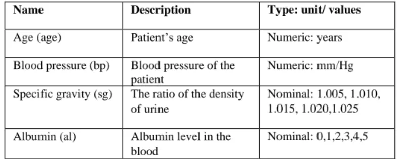
with outliers since these outliers could be legitimate (valid) or important. For this reason, each outlier detected in the CKD dataset is checked to know if it is realistic or not. In this study, the extreme data points that go beyond the acceptable range medically have been treated as missing data and then modified as will be described in the missing data section. Box plots have been used to detect outliers in the CKD dataset, As Fig. 1 shows, there are some outliers detected for blood glucose random that reached 500 mg/dl. However, as mentioned in [20], the highest blood glucose level recorded in 2008 for a surviving patient reached 2,656 mg/dl. So, these outliers are legitimate and we should not change them.

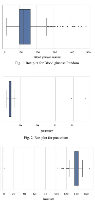
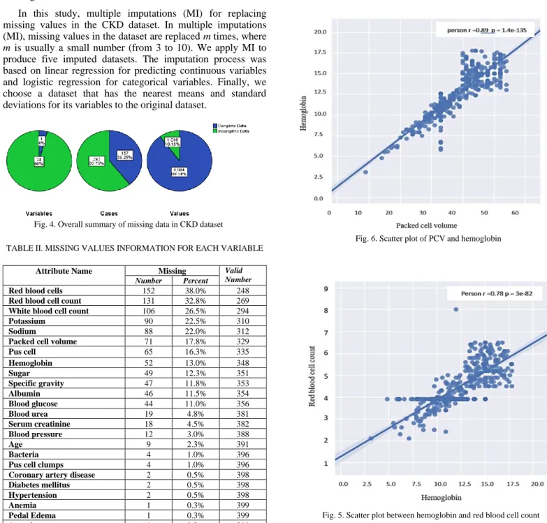
In contrast, for potassium and sodium, three extreme data points are unacceptable. The highest potassium level observed was 7.6 mEq/L [21]. This means that a potassium level with 39 and 47, as shown in Fig. 2 is impossible and usually due to a mistake. Similarly, with sodium, as Fig. 3 shows, one extreme data point was detected, which is 4.5. Normally, sodium level should be between 135 and 145 mEq/L, and if it is less than 135, then the patient suffers from hyponatremia [22]. For this reason, a value of 4.5 is unacceptable or impossible.

Fig. 1. Box plot for Blood glucose Random

Fig. 3. Box plot for Sodium Fig. 2. Box plot for potassium

4 | P a g e 2) Missing Values: In real-world datasets, missing data is a

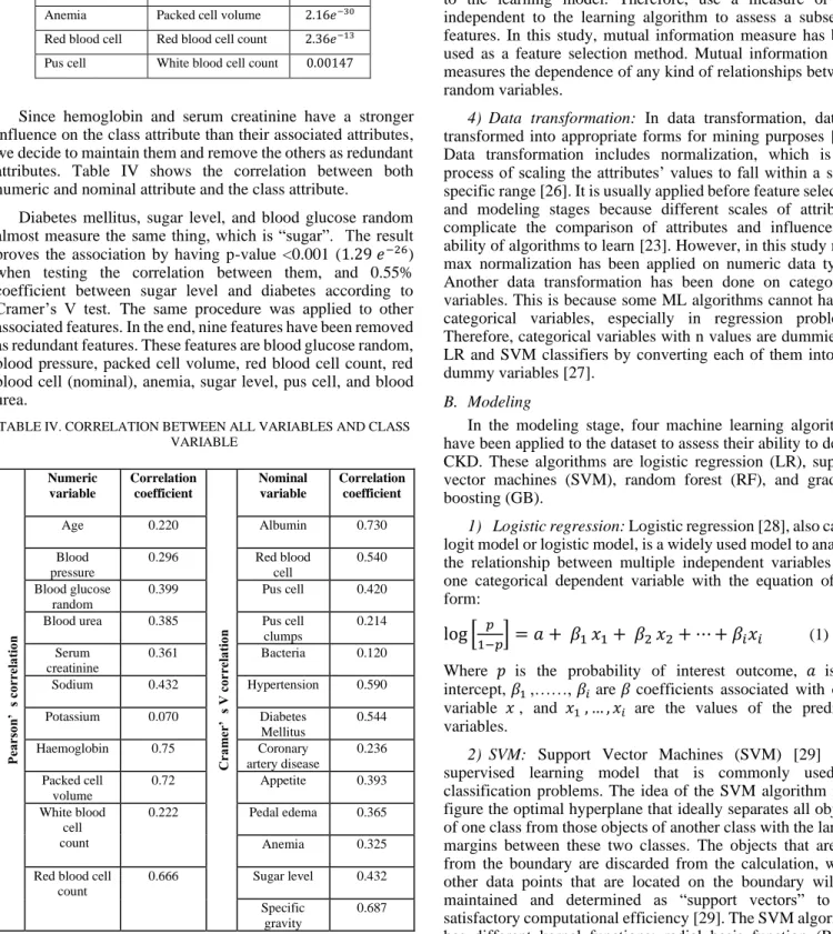
very common issue, especially in the medical area. Usually, every patient record and every attribute contains some missing values [23]. However, the chronic kidney disease dataset as shown in Fig. 4 has 96% of its variables having missing values; 60.75% (243) cases have at least one missing value, and 10% of all values are missing. There are different percentages of missing values for each variable, starting from 0.3% and reaching 38%, as shown in Table II.

Researchers in [9] used single imputation, such as mean and median, to impute the CKD dataset. However, according to Little’s test [24], the missing values in CKD dataset are not missing completely at random (MCAR) with p-value <0.005. Therefore, single imputation cannot be used for handling missing values.

In this study, multiple imputations (MI) for replacing missing values in the CKD dataset. In multiple imputations (MI), missing values in the dataset are replaced m times, where m is usually a small number (from 3 to 10). We apply MI to produce five imputed datasets. The imputation process was based on linear regression for predicting continuous variables and logistic regression for categorical variables. Finally, we choose a dataset that has the nearest means and standard deviations for its variables to the original dataset.

TABLE II. MISSING VALUES INFORMATION FOR EACH VARIABLE

3) Data Reduction: Data reduction means to reduce the number of features while maintaining a good analytical result. For this purpose, feature selection and features associations or correlation have been studied to remove redundant information.

a)Feature Associations: Pearson’s correlation, Cramer’s V, and ANOVA tests have been used to find relationships between variables. As shown in Fig. 5, and Fig. 6, there is a strong relationship between packed cell volume and hemoglobin and between hemoglobin and red cell count with the correlation coefficient of 0.89 and 0.79 respectively. Moreover, according to the ANOVA test, as shown in Table III, anemia also associated with PCV with p-value <0.001 (2.16𝑒−30_{). Another positive relationship was detected with a} correlation coefficient of 0.68 between blood urea and serum creatinine.

Attribute Name Missing Valid

Number

Number Percent

Red blood cells 152 38.0% 248

Red blood cell count 131 32.8% 269

White blood cell count 106 26.5% 294

Potassium 90 22.5% 310

Sodium 88 22.0% 312

Packed cell volume 71 17.8% 329

Pus cell 65 16.3% 335 Hemoglobin 52 13.0% 348 Sugar 49 12.3% 351 Specific gravity 47 11.8% 353 Albumin 46 11.5% 354 Blood glucose 44 11.0% 356 Blood urea 19 4.8% 381 Serum creatinine 18 4.5% 382 Blood pressure 12 3.0% 388 Age 9 2.3% 391 Bacteria 4 1.0% 396

Pus cell clumps 4 1.0% 396

Coronary artery disease 2 0.5% 398

Diabetes mellitus 2 0.5% 398

Hypertension 2 0.5% 398

Anemia 1 0.3% 399

Pedal Edema 1 0.3% 399

Appetite 1 0.3% 399

Fig. 6. Scatter plot of PCV and hemoglobin

Fig. 5. Scatter plot between hemoglobin and red blood cell count Fig. 4. Overall summary of missing data in CKD dataset

TABLE III. ANOVA TEST RESULTS

Since hemoglobin and serum creatinine have a stronger influence on the class attribute than their associated attributes, we decide to maintain them and remove the others as redundant attributes. Table IV shows the correlation between both numeric and nominal attribute and the class attribute.

Diabetes mellitus, sugar level, and blood glucose random almost measure the same thing, which is “sugar”. The result proves the association by having p-value <0.001 (1.29𝑒−26₎ when testing the correlation between them, and 0.55% coefficient between sugar level and diabetes according to Cramer’s V test. The same procedure was applied to other associated features. In the end, nine features have been removed as redundant features. These features are blood glucose random, blood pressure, packed cell volume, red blood cell count, red blood cell (nominal), anemia, sugar level, pus cell, and blood urea.

TABLE IV. CORRELATION BETWEEN ALL VARIABLES AND CLASS VARIABLE

b)Feature Selection: The process of selecting the most discriminating features in a given dataset is known as feature selection. This process is enhancing the model’s performance, reducing overfitting, and reducing the cost of building a model. Filter feature selection methods [25] selects features that have a stronger relationship with the outcome variable independent to the learning model. Therefore, use a measure or test independent to the learning algorithm to assess a subset of features. In this study, mutual information measure has been used as a feature selection method. Mutual information [25] measures the dependence of any kind of relationships between random variables.

4) Data transformation: In data transformation, data is transformed into appropriate forms for mining purposes [26]. Data transformation includes normalization, which is the process of scaling the attributes’ values to fall within a small specific range [26]. It is usually applied before feature selection and modeling stages because different scales of attributes complicate the comparison of attributes and influence the ability of algorithms to learn [23]. However, in this study min-max normalization has been applied on numeric data types. Another data transformation has been done on categorical variables. This is because some ML algorithms cannot handle categorical variables, especially in regression problems. Therefore, categorical variables with n values are dummied in LR and SVM classifiers by converting each of them into n-1 dummy variables [27].

B. Modeling

In the modeling stage, four machine learning algorithms have been applied to the dataset to assess their ability to detect CKD. These algorithms are logistic regression (LR), support vector machines (SVM), random forest (RF), and gradient boosting (GB).

1) Logistic regression: Logistic regression [28], also called logit model or logistic model, is a widely used model to analyze the relationship between multiple independent variables and one categorical dependent variable with the equation of the form:

log [

1−𝑝

] = 𝑎 + 𝛽

𝑥

+ 𝛽

𝑥

+ ⋯ + 𝛽

𝑥

Where 𝑝 is the probability of interest outcome, 𝑎 is an intercept, 𝛽1 ,……, 𝛽𝑖 are 𝛽 coefficients associated with each variable 𝑥, and 𝑥1 , … , 𝑥𝑖 are the values of the predictor variables.

2) SVM: Support Vector Machines (SVM) [29] is a supervised learning model that is commonly used in classification problems. The idea of the SVM algorithm is to figure the optimal hyperplane that ideally separates all objects of one class from those objects of another class with the largest margins between these two classes. The objects that are far from the boundary are discarded from the calculation, while other data points that are located on the boundary will be maintained and determined as “support vectors” to get satisfactory computational efficiency [29]. The SVM algorithm has different kernel functions: radial basis function (RBF), linear, sigmoid, and polynomial. In this study, radial basis Feature 1

Categorical

Feature 2 Numeric

P- value Diabetes mellitus Blood glucose random 1.29𝑒−26

Sugar level Blood glucose random 2.40𝑒−49

Hypertension Blood pressure 6.13𝑒−0.8

Anemia Packed cell volume 2.16𝑒−30

Red blood cell Red blood cell count 2.36𝑒−13

Pus cell White blood cell count 0.00147

Pe ar so n’ s co rr el at io n Numeric variable Correlation coefficient C ra m er ’ s V co rr el at io n Nominal variable Correlation coefficient Age 0.220 Albumin 0.730 Blood pressure 0.296 Red blood cell 0.540 Blood glucose random 0.399 Pus cell 0.420 Blood urea 0.385 Pus cell

clumps 0.214 Serum creatinine 0.361 Bacteria 0.120 Sodium 0.432 Hypertension 0.590 Potassium 0.070 Diabetes Mellitus 0.544 Haemoglobin 0.75 Coronary artery disease 0.236 Packed cell volume 0.72 Appetite 0.393 White blood cell count 0.222 Pedal edema 0.365 Anemia 0.325 Red blood cell

count

0.666 Sugar level 0.432 Specific

gravity

6 | P a g e function has been chosen based on nested cross-validation

results.

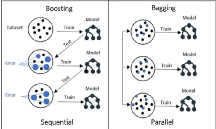
3) Ensemble method: Ensemble method [30] is a strategy for improving predictor or classifier accuracy. Ensemble method uses a combination of models to create an improved composite model to improve the performance. The main idea behind the ensemble technique is to group multiple “weak learners” to come up with a “strong learner”. Two popular techniques for constructing ensembles are bagging and boosting. Both boosting and bagging can be used for prediction as well as classification [26, 30]. Bagging is an ensemble technique where many independent predictors or learners are built and their results are combined using the majority vote, whereas in boosting, the predictors or learners are made sequentially not independently. This sequential method because each classifier “pays more attention” to the training tuples that were misclassified by the previous classifier through assigning weights for each of them [26]. Random forest algorithm is an example of the “bagging” technique, whereas the gradient boosting algorithm is an example of the “boosting” technique. Fig. 7 shows the bagging and boosting structure in selecting samples for training.

a)Random Forest: Random forest (RF) is a bagging ensemble approach proposed by Breiman [31] that based on a machine learning mechanism called “decision tree”. In a random forest, the “weak learners” in ensemble terms are decision trees [8, 32, 33]. Random forest imposes the diversity of each tree separately by selecting a random feature. After generating a large number of trees, they vote for the most common class. The random forest algorithm can deal with unbalanced data, it is robust against overfitting, and its runtimes are quite a bit faster [8, 31].

b)Gradient Boosting: Gradient boosting (GB) is an ensemble boosting technique that starts with “regression tree” as “weak learners”. In general, the GB model adds an additive model to minimize the loss function by using a stage-wise sampling strategy. The loss function measures the amount at which the expected value deviates from the real value. Stage-wise fashion put more emphasis on samples that are difficult to predict or misclassified. Unlike random forest, in GB, samples that are misclassified have a higher chance of being selected in training data [34]. GB reduces bias and variance and often provides higher accuracy, but the parameters should be tuned carefully to avoid overfitting. Therefore, nested cross-validation has been applied.

V. RESULTS AND DISCUSSION

The result of each classifier has been evaluated using different evaluation metrics and validated against overfitting using 10-fold cross-validation. The nested cross-validation approach also has been applied for the purpose of tuning the models’ parameters. The experiments are conducted using Python 3.3 programming language through the Jupyter Notebook web application. Several libraries from Sciket-learn [35] have been used, which is a free software for the machine learning library in Python. The evaluation measures considered in this study are accuracy using F1-measure, sensitivity, specificity, and area under the curve (AUC).

Each model generates different outputs depending on the different values of its parameters. By using nested cross-validation, the best performance for LR was with C=1000 and penalty=L2 with an accuracy of 98.9% using F1 measure. For the SVM model different values of “C”, “gamma”, and “kernel” have been tested. The best performance for SVM was with C=1 and gamma=3, and kernel = “RBF” (radial basis function) with an accuracy of 97.9% using F1 measure. For both RF and GB, the best results were with a number of trees=50 and Max_depth=2, with an accuracy of 98.0% in RF and 99.1% in GB using F1 measure.

The experimental results of each model in terms of accuracy, F1-measure, precision, sensitivity, specificity, AUC are listed in Table V. Whereas the training and testing accuracies based on 10-fold cross-validation are listed in Table VI.

Table V. THE PREDICTIVE PERFORMANCE OF ML MODELS

Classifier Accuracy F1 Precision Sensitivity Specificity AUC

Logistic regression 98.75% 98.9 % 99.5 % 98.4 % 99.33 % 99.7 %

Support victor machines 97.5% 97.9 % 99.5% 96.4 % 99.33% 99.9 %

Random forest 98.5% 98.7% 98.0% 99.6% 96.6% 99.5%

Gradient boosting 99.0% 99.1 % 99.5% 98.8 % 99.33% 99.9%

TABLE VI. THE TRAIN AND TEST ACCURACIES OF ML MODELS

From the evaluation results, as Fig. 8 shows, all models have an excellent performance against detecting CKD with an accuracy > 97% using hemoglobin, specific gravity, and albumin features. By focusing on specificity and sensitivity, it is seen that all models also have the same specificity of 99.3% except RF (96.6), which means that all models were accurate in identifying the negative or healthy subjects. On the other hand, the highest sensitivity was obtained using the RF algorithm at 99.6%, which represents the percentage of correctly identified CKD patients.

Hence, we achieve the highest detection performance with the GB model. This performance is higher than the performance achieved by [12] using a multilayer perceptron algorithm (MLP), seven features, and single-point split with 98.4% F1- measure. Also, higher performance Compared to study [8], were 98.0% F1-measure have been achieved using RF and five features. According to study [8], which also estimated the cost of each of 24 tests in the CKD dataset, performing these three features for detecting CKD would cost only $26.65 while using all features will cost around $451.36.

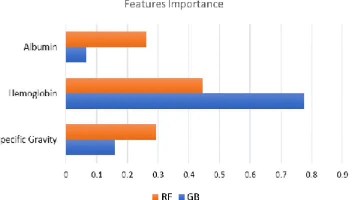
Since the higher results were achieved using RF, and GB algorithm, we also investigate the importance of the features in each of them. As shown in Fig. 9, hemoglobin has the highest score, whereas Albumin has the lowest score in both RF and GB. Looking at RF, the degree of importance is convergent for all variables, approximately from 0.29 to 0.44. Whereas in GB, there is a significant difference between the degree of importance of hemoglobin (0.77) and other features. Then, according to our result, we conclude that hemoglobin has played an essential role in detecting CKD.

However, this research is subject to some limitations related to the dataset used. First, the size of the dataset is considered to be small (400 instances), which may influence the reliability of the results. Second, difficulty finding another dataset that has the same features in order to compare the results of the datasets.

VI. CONCLUSION AND FUTURE WORK

This work examines the ability to detect CKD using machine learning algorithms while considering the least number of tests or features. We approach this aim by applying four machine learning classifiers: logistic regression, SVM, random forest, and gradient boosting on a small dataset of 400 records. In order to reduce the number of features and remove redundancy, the association between variables have been studied. A filter feature selection method has been applied to the remaining attributes and found that there are hemoglobin, albumin, and specific gravity have the most impact to predict the CKD.

The classifiers have been trained, tested, and validated using 10-fold cross-validation. Higher performance was achieved with the gradient boosting algorithm by F1-measure (99.1 %), sensitivity (98.8%), and specificity (99.3%). This result is the highest among previous studies with less number of features and hence less cost. Therefore, we conclude that CKD can be detected with only three features. Also, we found that hemoglobin has the highest contribution in detecting CKD, whereas albumin has the lowest using RF and GB models.

Since the data used in this research is small, in the future, we aim to validate our results by using big dataset or compare the results using another dataset that contains the same features. Also, in order to help in reducing the prevalence of CKD, we plan to predict if a person with CKD risk factors such as diabetes, hypertension, and family history of kidney failure will have CKD in the future or not by using appropriate dataset

.

ACKNOWLEDGMENT

This publication has emanated from research supported in part by a research grant from Science Foundation Ireland (SFI) under Grant Number SFI/12/RC/2289_P2, co-funded by the European Regional Development Fund. Special thanks to the deanship of scientific research at Princess Nourah bint Abdulrahman University for supporting this work.

REFERENCES

[1] J. Radhakrishnan et al, "Taming the chronic kidney disease epidemic: a global view of surveillance efforts," Kidney Int., vol. 86, (2), pp. 246-250, 2014.

[2] R. Lozano et al, "Global and regional mortality from 235 causes of death for 20 age groups in 1990 and 2010: a systematic analysis for the Global

LR SVM RF GB

Train 99.4 % 97.52% 98.5% 99.7%

Test 98.75 % 97.5% 98.5% 99.0%

Fig. 8. Models evaluation in predicting CKD

8 | P a g e Burden of Disease Study 2010," The Lancet, vol. 380, (9859), pp.

2095-2128, 2012.

[3] R. Ruiz-Arenas et al, "A Summary of Worldwide National Activities in Chronic Kidney Disease (CKD) Testing," Ejifcc, vol. 28, (4), pp. 302, 2017.

[4] Q. Zhang and D. Rothenbacher, "Prevalence of chronic kidney disease in population-based studies: systematic review," BMC Public Health, vol. 8,

(1), pp. 117, 2008.

[5] T. Di Noia et al, "An end stage kidney disease predictor based on an artificial neural networks ensemble," Expert Syst. Appl., vol. 40, (11), pp. 4438-4445, 2013.

[6] H. S. Chase et al, "Presence of early CKD-related metabolic complications predict progression of stage 3 CKD: a case-controlled study," BMC Nephrology, vol. 15, (1), pp. 187, 2014.

[7] K. A. Padmanaban and G. Parthiban, "Applying Machine Learning Techniques for Predicting the Risk of Chronic Kidney Disease," Indian Journal of Science and Technology, vol. 9, (29), 2016.

[8] A. Salekin and J. Stankovic, "Detection of chronic kidney disease and selecting important predictive attributes," in Healthcare Informatics (ICHI), 2016 IEEE International Conference On, 2016, .

[9] W. Gunarathne, K. Perera and K. Kahandawaarachchi, "Performance evaluation on machine learning classification techniques for disease classification and forecasting through data analytics for chronic kidney disease (CKD)," in Bioinformatics and Bioengineering (BIBE), 2017 IEEE 17th International Conference On, 2017, .

[10] H. Polat, H. D. Mehr and A. Cetin, "Diagnosis of chronic kidney disease based on support vector machine by feature selection methods," J. Med. Syst., vol. 41, (4), pp. 55, 2017.

[11] P. Yildirim, "Chronic kidney disease prediction on imbalanced data by multilayer perceptron: Chronic kidney disease prediction," in Computer Software and Applications Conference (COMPSAC), 2017 IEEE 41st Annual, 2017, .

[12] A. J. Aljaaf et al, "Early prediction of chronic kidney disease using machine learning supported by predictive analytics," in 2018 IEEE Congress on Evolutionary Computation (CEC), 2018, .

[13] J. Xiao et al, "Comparison and development of machine learning tools in the prediction of chronic kidney disease progression," Journal of Translational Medicine, vol. 17, (1), pp. 119, 2019.

[14] P. Yang et al, "A review of ensemble methods in bioinformatics," Current Bioinformatics, vol. 5, (4), pp. 296-308, 2010.

[15] L. Deng et al, "Prediction of protein-protein interaction sites using an ensemble method," BMC Bioinformatics, vol. 10, (1), pp. 426, 2009. [16] M. Fatima and M. Pasha, "Survey of machine learning algorithms for

disease diagnostic," Journal of Intelligent Learning Systems and Applications, vol. 9, (01), pp. 1, 2017.

[17] S. Karamizadeh et al, "Advantage and drawback of support vector machine functionality," in 2014 International Conference on Computer, Communications, and Control Technology (I4CT), 2014, .

[18] L. Rubini. (2015). Chronic_Kidney_Disease DataSet, UCI Machine

Learning Repository. Available:

https://archive.ics.uci.edu/ml/datasets/Chronic_Kidney_Disease. [19] J. D. Kelleher, B. Mac Namee and A. D'arcy, Fundamentals of Machine

Learning for Predictive Data Analytics: Algorithms, Worked Examples, and Case Studies. MIT Press, 2015.

[20] Michael and B. (2015). Highest blood sugar level. Available: http://www.guinnessworldrecords.com/world-records/highest-blood-sugar-level/.

[21] G. Gheno et al, "Variations of serum potassium level and risk of hyperkalemia in inpatients receiving low-molecular-weight heparin,"

Eur. J. Clin. Pharmacol., vol. 59, (5-6), pp. 373-377, 2003.

[22] D. A. Henry, "In The Clinic: Hyponatremia," Ann. Intern. Med., vol. 163,

(3), pp. ITC1-ITC19, 2015. DOI: 10.7326/AITC201508040.

[23] A. J. M. Kaky, "Intelligent Systems Approach for Classification and Management of Patients with Headache," Liverpool John Moores University, 2017.

[24] R. J. Little, "A test of missing completely at random for multivariate data with missing values," Journal of the American Statistical Association,

vol. 83, (404), pp. 1198-1202, 1988.

[25] J. R. Vergara and P. A. Estévez, "A review of feature selection methods based on mutual information," Neural Computing and Applications, vol. 24, (1), pp. 175-186, 2014.

[26] J. Han, J. Pei and M. Kamber, Data Mining: Concepts and Techniques.

Elsevier, 2011.

[27] M. A. Hardy, Regression with Dummy Variables. Sage, 1993(93).

[28] J. V. Tu, "Advantages and disadvantages of using artificial neural networks versus logistic regression for predicting medical outcomes," J. Clin. Epidemiol., vol. 49, (11), pp. 1225-1231, 1996.

[29] Z. Chen, X. Zhang and Z. Zhang, "Clinical risk assessment of patients with chronic kidney disease by using clinical data and multivariate models,"

Int. Urol. Nephrol., vol. 48, (12), pp. 2069-2075, 2016.

[30] T. G. Dietterich, "An experimental comparison of three methods for constructing ensembles of decision trees: Bagging, boosting and randomization," Mach. Learning, vol. 32, pp. 1-22, 1998.

[31] L. Breiman, "Random Forests," Mach. Learning, vol. 45, (1), pp. 5-32, 2001.

[32] T. G. Dietterich, "Ensemble methods in machine learning," in

International Workshop on Multiple Classifier Systems, 2000, . [33] M. Khalilia, S. Chakraborty and M. Popescu, "Predicting disease risks

from highly imbalanced data using random forest," BMC Medical Informatics and Decision Making, vol. 11, (1), pp. 51, 2011.

[34] Y. Zhang and A. Haghani, "A gradient boosting method to improve travel time prediction," Transportation Research Part C, vol. 58, pp. 308-324, 2015.

[35] F. Pedregosa et al, "Scikit-learn: Machine learning in Python," Journal of Machine Learning Research, vol. 12, (Oct), pp. 2825-2830, 2011.