Sharif University of Technology
Scientia Iranica
Transactions A: Civil Engineering
www.sciencedirect.com
Utilization of a least square support vector machine (LSSVM) for
slope stability analysis
P. Samui
a,∗,
D.P. Kothari
baCentre for Disaster Mitigation and Management, VIT University, Vellore-632014, India bVindhya Institute of Technology & Science, Indore, India
Received 18 July 2010; revised 22 October 2010; accepted 20 December 2010
KEYWORDS Slope stability;
Least square support vector machine;
Artificial neural network; Probability;
Prediction.
Abstract This paper examines the capability of a least square support vector machine (LSSVM) model for slope stability analysis. LSSVM is firmly based on the theory of statistical learning, using regression and classification techniques. The Factor of Safety (FS) of the slope has been modelled as a regression problem, whereas the stability status (s) of the slope has been modelled as a classification problem. Input parameters of LSSSVM are: unit weight(γ ), cohesion(c), angle of internal friction(φ), slope angle(β), height(H)and pore water pressure coefficient (ru). The developed LSSVM also gives a probabilistic output. Equations have also been developed for the slope stability analysis. A comparative study has been carried out between the developed LSSVM and an artificial neural network (ANN). This study shows that the developed LSSVM is a robust model for slope stability analysis.
©2011 Sharif University of Technology. Production and hosting by Elsevier B.V.
1. Introduction
The analysis of slope stability is an imperative task in the design and construction of different civil engineering struc-tures, such as highways, open pits, earth dams etc. Geotech-nical engineers use different methods for slope stability analysis, such as limit equilibrium [1–4], upper bound limit analysis [5–12], finite element [13,14], maximum likelihood [15], genetic programming [16] etc. The artificial neural net-work (ANN) has been successfully adopted in the slope stability problem [17,18]. However, ANN has some limitations, such as arriving at local minima, a low convergence speed, a black box approach and a lesser generalization performance [19,20].
This study employs the least square support vector machine (LSSVM) for prediction of the Factor of Safety (FS), which has
∗Corresponding author.
E-mail address:[email protected](P. Samui).
been modeled as a regression problem, and the stability status (s) of the slope, which has been modeled as a classification problem. LSSVM is a statistical learning theory that adopts a least squares linear system as a loss function [21]. LSSVM is closely related to regularization networks [22]. With the quadratic cost function, the optimization problem reduces to find the solution of a set of linear equations. The data have been taken from the work of Sakellatiou and Ferentinou [17]. The dataset contains information about unit weight (d), cohesion (c), angle of internal friction (
φ
), slope angle (β
), height (H), pore water pressure coefficient (ru),FSands. The paper has thefollowing aims:
1. To examine the feasibility of LSSVM for slope stability analysis;
2. To determine probabilistic output;
3. To develop equations for slope stability analysis;
4. To make a comparative study between the developed LSSVM model and the ANN model developed by Sakellatiou and Ferentinou [17].
2. LSSVM for classification
This section of the paper serves as an introduction to LSSVM. Details of this method can be found in Suykens et al. [23]. A binary classification problem is considered, having a set of training vectors (D) belonging to two separate classes.
D
=
(
x1,
y1), . . . , (
xl,
yl)
,
x∈
Rn,
y∈ {−1
,
+1}
,
(1)1026-3098©2011 Sharif University of Technology. Production and hosting by
doi:10.1016/j.scient.2011.03.007
Open access under CC BY license.
Elsevier B.V.
Peer review under responsibility of Sharif University of Technology.
wherex
∈
Rnis ann-dimensional data vector, with each samplebelonging to either of two classes labelledy
∈ {−1
,
+1}, and l is
the number of training data. This study usesd,c,φ
,β
,Handruas input parameters. Sox
= [
d,
c, β, φ,
ru,H]. In the current
context of classifying the status of the slope, the two classes labeled+1 and
−1 may mean stable slope and failed slope. The
Support Vector Machine (SVM) approach aims at constructing a classifier of the form:y
(
x)
=
sign
N−
k=1αk
ykk(
x,
xk)+
b
,
(2)where
αk
are positive real constants,bis the scalar threshold,Nis the number of the dataset andk
(
x,
xk)is the Kernel function. For the case of two classes, one assumes:w
Tϕ(
xk)+
b≥
1,
ifyk
= +1
(
stable slope),
w
Tϕ(
xk)+
b≤
1,
ifyk
= −1
(
failed slope),
(3)where
w
is an adjustable weight vector,Tis the transpose andϕ(.)
is the feature map that maps the input space into a higher dimensional space, which is equivalent to:yk
w
Tϕ(
xk)+
b
≥
1,
k=
1, . . . ,
N.
(4)According to the structural risk minimization principle, the risk bound is minimized by formulating the following optimization problem [24]: Minimize:1 2
w
Tw
+
γ
2 l−
k=1 e2k, Subjected to:yk
w
Tϕ(
xk)+
b
=
1−
ek, k=
1, . . . ,
N,
(5) whereγ
is the regularization parameter, determining the trade-off between the fitting error minimization and smoothness, andekis error variable. This optimization problem (Eq.(5)) is solved
by Lagrange multipliers [21], and its solution is given by:
y
(
x)
=
sign
N−
k=1αk
ykK(
x,
xk)+
b
,
(6)where sign () is the signum function. It gives
+1 (stable slope)
if the element is greater than or equal to zero, and−1 (failed
slope) if it is less than zero.This study adopts the above methodology for prediction of ‘s’ of the slope. The dataset consists of 46 case studies of slopes. To use these data for classification purposes, a value of 1 is assigned to the stable condition of the slope, while a value of
−1 is assigned to the failure condition of the slope so as to make
this a two-class classification problem. In this model,d,c,φ
,β
,H, andruare used as input parameters. The data are normalized
between 0 to 1. In carrying out the formulation, the data have been divided into two sub-sets, such as:
(a) A training dataset: This is required to construct the model. In this study, 32 out of 46 data are considered for the training dataset.
(b) A testing dataset: This is required to estimate the model performance. In this study, the remaining 14 data are considered as a testing dataset. To train the LSSVM model, a radial basis function has been used as a Kernel function. The program of the classification problem is constructed using MATLAB.
3. LSSVM for regression
LSSVM models are an alternate formulation of SVM regres-sion [25], proposed by Suykens et al. [23]. Consider a given training set ofNdata points,
{
xk,yk}
kN=1, with input dataxk∈
RN,and outputyk
∈
r, whereRNis theN-dimensional vector spaceand r is the one-dimensional vector space. For a regression problem, the same input variables are employed as used in the classification problem. The output of the LSSVM model isFS. So, in this studyx
= [
d,
c, β, ϕ,
ru,H]
andy=
FS. In feature space, LSSVM models take the form:y
(
x)
=
w
Tϕ(
x)
+
b,
(7)where the feature map
ϕ(.)
maps the input data into a higher dimensional feature space;w
∈
Rn;b∈
r;w
=
an adjustableweight vector; andb
=
the scalar threshold. In LSSVM, for function estimation, the following optimization problem is formulated: Minimize: 1 2w
Tw
+
1 2 N−
k=1 e2k, Subject to:y(
x)
=
w
Tϕ(
xk)+
b+
ek, k=
1, . . . ,
N,
(8) whereNis the number of data.The following equation forFSprediction has been obtained by solving the above optimization problem [26,27]:
FS
=
y(
x)
=
N
−
k=1
αk
K(
x,
xk)+
b.
(9)The radial basis function has been used in this analysis, and is given by: K
(
xk,xl)=
exp
−
(
xk−
xl) T(
x k−
xl) 2σ
2
,
k,
l=
1, . . . ,
N,
(10) whereσ
is the width of the radial basis function.This study examines the capability of the above method-ology for prediction ofFS. The same training dataset, testing dataset and normalization technique have been adopted as used in the classification problem. The program of the classification problem is constructed using MATLAB.
4. Results and discussion
The design values of
γ
andσ
have been determined by a trial and error approach. The training and testing performance has been calculated using the following formula:Training performance (%) or Testing performance (%)
=
No of data predicted accurately by LSSVM Total data
×
100
.
(11) The design values ofγ
andσ
are 80 and 30, respectively. The training performance has been determined by using the design values ofγ
andσ
and is 100%. Therefore, the developed LSSVM models have successfully captured the input and output relationship. Now, the developed LSSVM model has been used to determine the performance of the testing dataset. Only one data has been misclassified for testing the dataset. Therefore, the testing performance is 92.85%. The developed LSSVM modelTable 1: Performance of training dataset for prediction ofsof slope.
d(kN/m3) c(kPa) ϕ(°) β(°) H(m) r
u Actual class Predicted class Values ofαfor classification Values ofαfor regression 18.68 26.34 15 35 8.23 0 −1 −1 0.78 −4.33 16.5 11.49 0 30 3.66 0 −1 −1 −8.30 6.71 18.84 14.36 25 20 30.5 0 1 1 9.72 3.35 28.44 29.42 35 35 100 0 1 1 17.82 0.63 28.44 39.23 38 35 100 0 1 1 −6.43 6.06 14.8 0 17 20 50 0 −1 −1 39.00 −6.91 14 11.97 26 30 88 0 −1 −1 −5.35 −2.16 25 120 45 53 120 0 1 1 4.07 −1.15 26 150.05 45 50 200 0 1 1 −3.37 −5.75 18.5 12 0 30 6 0 −1 −1 −4.23 5.49 22.4 10 35 30 10 0 1 1 −22.52 −0.17 21.1 10 30.34 30 20 0 1 1 29.54 −9.11 22 0 36 45 50 0 −1 −1 14.38 −2.32 12 0 30 35 4 0 1 1 26.99 0.61 12 0 30 35 4 0 1 1 26.99 0.88 12 0 30 45 8 0 −1 −1 36.44 1.57 23.47 0 32 37 214 0 −1 −1 0.95 4.44 19.63 11.97 20 22 12.19 0.405 −1 −1 14.69 −11.98 21.82 8.62 32 28 12.8 0.49 −1 −1 52.76 6.54 18.84 0 20 20 7.62 0.45 −1 −1 28.29 −5.97 21.43 0 20 20 61 0.5 −1 −1 −19.47 2.39 19.06 11.71 28 35 21 0.11 −1 −1 41.37 −10.97 21.51 6.94 30 31 76.81 0.38 −1 −1 4.02 −3.27 18 24 30.15 45 20 0.12 −1 −1 −13.88 3.72 23 0 20 20 100 0.3 −1 −1 7.15 0.15 22.4 10 35 45 10 0.4 −1 −1 0.73 2.2 20 20 36 45 50 0.25 −1 −1 3.57 −1.74 20 20 36 45 50 0.5 −1 −1 −9.96 2.27 20 0 36 45 50 0.5 −1 −1 −8.18 −2.71 22 0 40 33 8 0.35 1 1 24.32 1.06 20 0 24.5 20 8 0.35 1 1 65.52 1.64 18 5 30 20 8 0.3 1 1 2.12 18.75
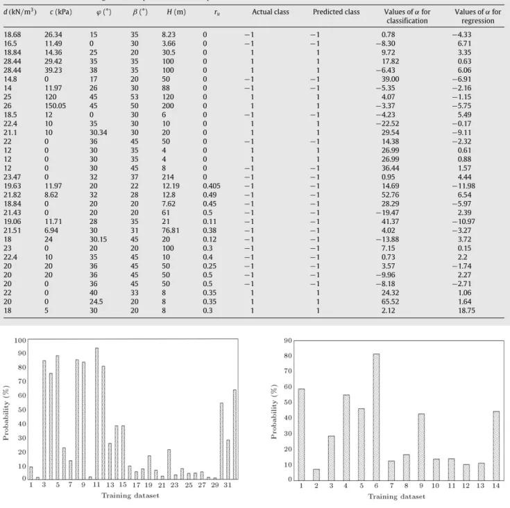
Figure 1: Probability of training dataset.
has been also used to determine the probability.Figures 1and
2 depict the probability of training and testing the dataset, respectively. These figures can be also used to predict the corresponding risk. The developed LSSVM model also gives the following equation (by puttingK
(
x,
xk)=
exp
−
(xk−x)T(xk−x) 2σ2
,
N
=
32,σ
=
30 andb=
1.
1432 in Eq.(6)) for determination of ‘s’ of the slope: s=
sign
32−
k=1αk
ykexp
−
(
xk−
x)
T(
x k−
x)
1800
+
1.
1432
.
(12) The values ofα
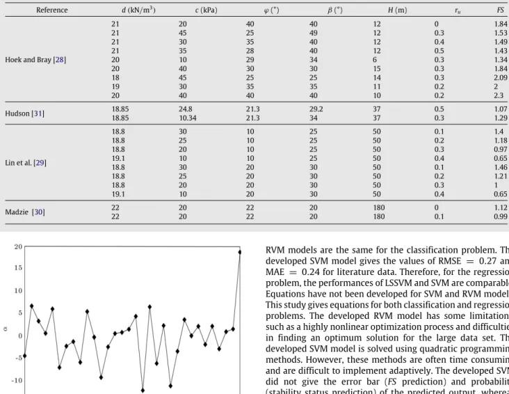
have been given inFigure 3andTable 1for the classification problem.Table 2shows the performance of the testing dataset.Figure 2: Probability of testing dataset.
For a regression problem, the design values of
γ
andσ
are 20 and 30, respectively. The performance of the training dataset has been determined using the design values ofγ
andσ
.Figure 4illustrates the performance of the training dataset. The value of R(
R=
0.
961)
is close to one for the training dataset. For a good model, the value ofR should be close to one. Therefore, the developed LSSVM model has successfully captured the input and output relations for the training dataset. Now, the performance of the developed LSSVM model has been examined for the testing dataset. Figure 5 depicts the performance of the testing dataset.Figure 5also confirms that the developed LSSVM model has the capability of predictingFS. Figures 6 and 7 show a 95% error bar for training and testing the dataset, respectively. The obtained error bar can be
Figure 3: Values ofαfor classification problem. Table 2: Performance of testing dataset for prediction ofsof slope.
d(kN/m3) c(kPa) ϕ(°) β(°) H(m) r u Actual class Predicted class 24 0 40 33 8 0.3 1 1 16 70 20 40 115 0 −1 −1 20.41 33.52 11 16 45.72 0.2 −1 −1 18.84 15.32 30 25 10.67 0.38 1 1 18.84 14.36 25 20 30.5 0.45 −1 −1 22.4 100 45 45 15 0.25 1 1 20 0 36 45 50 0.25 −1 −1 20.6 16.28 26.5 30 40 0 −1 −1 18.84 57.46 20 20 30.5 0 1 1 18.5 25 0 30 6 0 −1 −1 22 20 36 45 50 0 −1 −1 12 0 30 45 8 0 −1 −1 14 11.97 26 30 88 0.45 −1 −1 20.41 24.9 13 22 10.67 0.35 1 −1
Figure 4: Performance of training dataset.
used for determination of the confidence interval. The following equation (by puttingK
(
x,
xk)=
exp
−
(xk−x)T(xk−x) 2σ2
,N
=
32,σ
=
30 andb= −0
.
4386 in Eq.(9)) has been developed for the prediction ofFS: FS=
32−
k=1αk
exp
−
(
xk−
x)
T(
x k−
x)
1800
−
0.
4386.
(13)Figure 8andTable 1show the values of
α
forFSprediction.Figure 5: Performance of testing dataset.
Figure 6: 95% error bar for training dataset.
Figure 7: 95% error bar for testing dataset.
A comparative study has been carried out between the developed LSSVM forFSprediction and the ANN model [17]. The ANN model consists of one input layer, one hidden layer with six neurons and one output layer. The learning rate and error goal of the ANN model are 0.02 and 0.03, respectively. The data have been collected from the chart given by Hoek and Bray [28], Lin et al. [29], Madzie [30]and Hudson [31];
Table 3presents the dataset. Comparison has been done in terms of Root Mean Square Error (RMSE) and Mean Absolute
Table 3: Data from different literatures.
Reference d(kN/m3) c(kPa) ϕ(°) β(°) H(m) r
u FS
Hoek and Bray [28]
21 20 40 40 12 0 1.84 21 45 25 49 12 0.3 1.53 21 30 35 40 12 0.4 1.49 21 35 28 40 12 0.5 1.43 20 10 29 34 6 0.3 1.34 20 40 30 30 15 0.3 1.84 18 45 25 25 14 0.3 2.09 19 30 35 35 11 0.2 2 20 40 40 40 10 0.2 2.3 Hudson [31] 18.85 24.8 21.3 29.2 37 0.5 1.07 18.85 10.34 21.3 34 37 0.3 1.29 Lin et al. [29] 18.8 30 10 25 50 0.1 1.4 18.8 25 10 25 50 0.2 1.18 18.8 20 10 25 50 0.3 0.97 19.1 10 10 25 50 0.4 0.65 18.8 30 20 30 50 0.1 1.46 18.8 25 20 30 50 0.2 1.21 18.8 20 20 30 50 0.3 1 19.1 10 20 30 50 0.4 0.65 Madzie [30] 22 20 22 20 180 0 1.12 22 20 22 20 180 0.1 0.99
Figure 8: Values ofαforFSprediction. Table 4: Comparison between ANN and LSSVM models.
Model RMSE MAE
ANN 0.3743 0.3134
LSSVM 0.2840 0.2325
Error (MAE).Table 4shows the values of RMSE and MAE for ANN and LSSVM models. From Table 4, it is clear that the developed LSSVM model outperforms the ANN model. The LSSVM model uses only two parameters (
γ
andσ
), whereas ANN uses a number of hidden layers, a number of hidden nodes, a learning rate, a momentum term, a number of training epochs, transfer functions, and weight initialization methods. Obtaining an optimal combination of these parameters is also a difficult task.The results from the LSSVM model have been also compared with the SVM and the Relevance Vector Machine (RVM) developed by Samui [32] and Samui et al. [33]. For the classification problem, the performance of the LSSVM model is better than the SVM model. The performances of LSSVM and
RVM models are the same for the classification problem. The developed SVM model gives the values of RMSE
=
0.
27 and MAE=
0.
24 for literature data. Therefore, for the regression problem, the performances of LSSVM and SVM are comparable. Equations have not been developed for SVM and RVM models. This study gives equations for both classification and regression problems. The developed RVM model has some limitations, such as a highly nonlinear optimization process and difficulties in finding an optimum solution for the large data set. The developed SVM model is solved using quadratic programming methods. However, these methods are often time consuming and are difficult to implement adaptively. The developed SVM did not give the error bar (FS prediction) and probability (stability status prediction) of the predicted output, whereas the developed LSSVM does.5. Conclusion
The LSSVM for slope stability analysis has been described in this paper. Forty six data have been employed to construct the LSSVM model. The developed LSSVM has given encouraging results for prediction of the stability status of the slope, as well as the factor of safety. It also gives a probabilistic output. The performance of the developed LSSVM is found to be better than that of the ANN. The developed LSSVM model can be used as a quick tool for slope stability analysis without using any table or chart. The user can employ the developed equations for slope stability analysis. The developed LSSVM model can be used as a powerful tool for slope stability analysis.
References
[1] Fellenius, W. ‘‘Calculation of stability of earth dams’’,Transactions Second Congress on Large Dams, 4, Washington, p. 445 (1936).
[2] Bishop, A.W. ‘‘The use of slip circle in the stability of slopes’’,Geotechnique, 5(1), pp. 7–17 (1955).
[3] Bishop, A.W. and Morgenstern, N.R. ‘‘Stability coefficients for earth slopes’’,
Geotechnique,10(4), pp. 129–150 (1960).
[4] Morgenstern, N.R. and Price, V.E. ‘‘The analysis of the stability of general slip surfaces’’,Geotechnique,15(1), pp. 79–93 (1965).
[5] Chen, W.F., Giger, M.W. and Fang, H.Y. ‘‘On the limit analysis of stability of slopes’’,Soils and Foundations,9(4), pp. 23–32 (1969).
[6] Karal, K. ‘‘Energy method for soil stability analyses’’,Journal of Geotechnical Engineering ASCE,103(5), pp. 431–447 (1977).
[7] Karal, K. ‘‘Application of energy method’’,Journal of Geotechnical Engineer-ing Division ASCE,103(5), pp. 381–399 (1977).
[8] Chen, W.F. and Liu, X.L., Limit Analysis in Soil Mechanics, Elsevier, Amsterdam, (1990).
[9] Michalowski, R.L. ‘‘Limit analysis of slopes subjected to pore pressure’’, inProceeding, Conference on Comp. Methods and Advances in Geomech, Srirwardane and Zaman, Eds., Balkema, Rotterdam, Netherlands (1994). [10] Michalowski, R.L. ‘‘Slope stability analysis: a kinematical approach’’,
Geotechnique,45(2), pp. 283–293 (1995).
[11] Michalowski, R.L. ‘‘Stability charts for uniform slopes’’, Journal of Geotechnical and Geoenvironmental Engineering ASCE,128(4), pp. 351–355 (2002).
[12] Kumar, J. and Samui, P. ‘‘Determination for layered soil slopes using the upper bound limit analysis’’,Geotechnical and Geological Engineering,24(6), pp. 1803–1819 (2006).
[13] Zou, J.Z., Williams, D.J. and Xiong, W.L. ‘‘Search for critical slip surfaces based on finite element method’’,Canadian Geotechnical Journal,32(2), pp. 233–246 (1995).
[14] Griffiths, D.V. and Lane, P.A. ‘‘Slope stability analysis by finite elements’’,
Geotechnique,49(3), pp. 387–403 (1999).
[15] Sah, N.K., Sheorey, P.R. and Upadhyaya, L.N. ‘‘Maximum likelihood estimation of slope stability’’,International Journal of Rock Mechanics and Mining Sciences and Geomechanics,31(1), pp. 47–53 (1994).
[16] Yang, C.X., Tham, L.G., Feng, X.T., Wang, Y.J. and Lee, P.K.K. ‘‘Two-stepped evolutionary algorithm and its application to stability analysis of slopes’’,
Journal of Computing in Civil Engineering,18(2), pp. 145–153 (2004). [17] Sakellatiou, M.G. and Ferentinou, M.D. ‘‘A study of slope stability
prediction using neural networks’’,International Journal of Geotechnical and Geological Engineering,23, pp. 419–445 (2005).
[18] Samui, P. and Kumar, B. ‘‘Artificial neural network prediction of stability numbers for two-layered slopes with associated flow rule’’,Electronic Journal of Geotechnical Engineering,11, (2006).
[19] Park, D. and Rilett, L.R. ‘‘Forecasting freeway link travel times with a multi-layer feed forward neural network’’,Computer Aided Civil and Structure Engineering,14, pp. 358–367 (1999).
[20] Kecman, V., Learning and Soft Computing: Support Vector Machines, Neural Networks, and Fuzzy Logic Models, The MIT Press, Cambridge, Massachusetts, London, England, (2001).
[21] Suykens, J.A.K., Lukas, L., Van Dooren, P., De Moor, B. and Vandewalle, J. ‘‘Least squares support vector machine classifiers: a large scale algorithm’’, inProc. Eur. Conf. Circuit Theory and Design (ECCTD ’99), Stresa, Italy, pp. 839–842 (1999).
[22] Smola, A.J. ‘‘Learning with Kernels’’, Ph.D. Dissertation, GMD, Birlinghoven, Germany (1998).
[23] Suykens, J.A.K., De Brabanter, J., Lukas, L. and Vandewalle, J. ‘‘Weighted least squares support vector machines: robustness and sparse approxima-tion’’,Neurocomputing,48(1–4), pp. 85–105 (2002).
[24] Suykens, J.A.K. and Vandewalle, J. ‘‘Least squares support vector machine classifiers’’,Neural Processing Letters,9(3), pp. 293–300 (1999).
[25] Smola, A. and Scholkopf, B. ‘‘On a Kernel based method for pattern recogni-tion, regression, approximation and operator inversion’’,Algorithmica,22, pp. 211–231 (1998).
[26] Vapnik, V. and Lerner, A. ‘‘Pattern recognition using generalized portrait method’’,Automation and Remote Control,24, pp. 774–780 (1963). [27] Vapnik, V.N.,Statistical Learning Theory, Wiley, New York, (1998).
[28] Hoek, E. and Bray, J.W.,Rock Slope Engineering, 3rd Ed., Institution of Mining and Metallurgy, London, (1981).
[29] Lin, P.S., Lin, M.H. and Lee, T.M. ‘‘An investigation on the failure of a building constructed on hillslope’’, inBonnard (Ed.) Landslides, Balkema, 1, pp. 445–449 (1988).
[30] Madzie, E. ‘‘Stability of unstable final slope in deep open iron mine’’, in
Bonnard (Ed.) Landslides, Balkema, 1, pp. 455–458 (1988).
[31] Hudson, J.A.,Rock Engineering-Theory and Practice, Ellis Horwood Limited, West Sussex, (1992).
[32] Samui, P. ‘‘Slope stability analysis: a support vector machine approach’’,
Environmental Geology,56, pp. 255–267 (2008).
[33] Samui, P., Bhattocharya, G. and Das, S. ‘‘Support vector machine and relevance vector machine classifier in analysis of slopes’’, in12th Int. Conf. of Int. Assoc. for Comp. Methods and Advances in Geomechanics, Goa, India, pp. 4667–4674 (2008).
Pijush Samuiis Associate Professor in the Center for Disaster Mitigation and Management at the Vellore Institute of Technology, Vellore, India. He received his Ph.D. Degree from the Indian Institute of Science in Bangalore, India, in 2008. Dr. Samui’s research interests cover a wide range of subjects in Geotechnical Engineering, including: Application of Soft Computing in Civil Engineering, Numerical Modeling, Landslide, Risk and Reliability Analysis, Geostatistics, Slope Stability, Pile Foundation, Site Characterization, Rock Mechanics, Development of Different Experimental Devices and Modeling of Different Seismic Hazards. He has published and presented 60 technical papers in journals and at conferences. He is an elected Fellow member of the International Congress of Disaster Management and Earth Sciences, India. He also serves as an Editorial Board member of several international journals. Dwarkadas Pralhaddas Kothariobtained his B.E. in Electrical Engineering, M.E. in Power Systems and Ph.D. in Electrical Engineering from the Birla Institute of Technology & Science, in Pilani. His fields of specialization are: Optimal Hydro-thermal Scheduling, Unit Commitment, Maintenance Scheduling, Energy Conservation (loss minimization and voltage control), and Power Quality and Energy Systems Planning and Modelling. Prof. Kothari is the recipient of the National Khosla Lifetime Achievement Award (2005) from the Indian Institute of Technology, Roorkee, the National Award for Science and Technology (2001) from the UP Government at the annual convention of ISTE, Bhubaneswar, and the Eminent Engineering Personality award from the Institution of Engineers (2001). He has also won several best paper awards and gold medals for his work. Prior to his assuming charge as Vice Chancellor of VIT University, he was Professor at the Centre for Energy Studies, at the Indian Institute of Technology, New Delhi. He also served as Director i/c of IIT, Delhi (2005), Deputy Director (Administration) of IIT, Delhi (2003–06), Principal of Visvesvaryaya Regional Engineering College, Nagpur (1997–98), and Head of the Centre for Energy Studies, IIT, Delhi (1995–97).
He was visiting Professor at the Royal Melbourne Institute of Technology, Melbourne, Australia in 1982–83 and 1989 for two years, and NSF Fellow at Purdue University, USA, in 1992. Prof. Kothari has published 625 research papers in various national and international journals and conferences, supervised 27 Ph.D.s and 55 MTechs, and authored 20 books concerning Power Systems and other allied areas. He has also delivered several keynote addresses at both national and international conferences on Electric Energy Systems. Prof. Kothari is a Fellow of the Indian National Academy of Engineering (FNAE), Indian National Academy of Sciences (FNASc), Institution of Engineers (FIE) and senior member of the IEEE.