Understanding Model-Based Reinforcement Learning and its Application in Safe Reinforcement Learning

(1)

UC San Diego

UC San Diego Electronic Theses and Dissertations

Title

Understanding Model-Based Reinforcement Learning and its Application in Safe Reinforcement Learning Permalink https://escholarship.org/uc/item/3pp5r7w5 Author Hu, Dingcheng Publication Date 2019 Peer reviewed|Thesis/dissertation

(2)

UNIVERSITY OF CALIFORNIA SAN DIEGO

Understanding Model-Based Reinforcement Learning and its Application in Safe Reinforcement Learning

A Thesis submitted in partial satisfaction of the requirements for the degree

Master of Science in Computer Science by Dingcheng Hu Committee in charge:

Professor Sicun Gao, Chair Professor Kamalika Chaudhuri Professor Hao Su

(3)

Copyright Dingcheng Hu, 2019

(4)

The Thesis of Dingcheng Hu is approved, and it is accept-able in quality and form for publication on microfilm and electronically:

Chair

University of California San Diego

(5)

LIST OF FIGURES

Figure 3.1: Comparison between real cost and model cost in ME-TRPO . . . 15

Figure 3.2: Dynamics validation loss in ME-TRPO . . . 16

Figure 3.3: MBPO’s learning curve on HalfCheetah environment . . . 17

Figure 3.4: MBPO Dynamics validation loss . . . 17

Figure 4.1: Mixing safe and performant policy . . . 30

Figure 4.2: Three constrained environments . . . 31

Figure 4.3: Sample trajectories for the Reacher environment . . . 31

Figure 4.4: Sample trajectories for the Racecar environment . . . 32

Figure 4.5: Sample trajectories for the Ant environment . . . 33

Figure 4.6: Compares rewards and violations with CPO in Reacher, Racecar and Ant . 34 Figure 4.7: The true rewards in our algorithm . . . 35

Figure 4.8: Complexity of racecar, reacher and ant in our curriculum . . . 35

(7)

LIST OF TABLES

Table 3.1: Comparison between training loss and validation loss in various environments 11 Table 3.2: Performance of TRPO on model trained from 63000 randomly collected data

(8)

ACKNOWLEDGEMENTS

I would like to acknowledge Professor Sicun Gao for his support as the chair of my committee. I thank him for providing me an opportunity to do research in the field of artificial intelligence. His guidance has proved to be invaluable. I am grateful to Prof. Hao Su and Prof. Kamalika Chaudhuri for their time to review my research and their valuable comments. I would also like to thank my fellow UCSD classmate Chenghao Gong, who gave me suggestions on thesis preparation.

Chapter 4, in part, has been submitted for publication of the material. It is a joint work with Yixuan Huang, Zhi Wang, Yuda Song and Sicun Gao. The thesis author was a co-author of this material.

(9)

ABSTRACT OF THE THESIS

Understanding Model-Based Reinforcement Learning and its Application in Safe Reinforcement Learning

by

Dingcheng Hu

Master of Science in Computer Science

University of California San Diego, 2019

Professor Sicun Gao, Chair

Model-based reinforcement learning algorithms have been shown to achieve successful results on various continuous control benchmarks, but the understanding of model-based methods is limited. We try to interpret how model-based method works through novel experiments on state-of-the-art algorithms with an emphasis on the model learning part. We evaluate the role of the model learning in policy optimization and propose methods to learn a more accurate model. With a better understanding of model-based reinforcement learning, we then apply model-based methods to solve safe reinforcement learning (RL) problems with near-zero violation of hard constraints throughout training. Drawing an analogy with how humans and animals learn to

(10)

perform safe actions, we break down the safe RL problem into three stages. First, we train agents in a constraint-free environment to learn a performant policy for reaching high rewards, and simultaneously learn a model of the dynamics. Second, we use model-based methods to plan safe actions and train a safeguarding policy from these actions through imitation. Finally, we propose a factored framework to train an overall policy that mixes the performant policy and the safeguarding policy. This three-step curriculum ensures near-zero violation of safety constraints at all times. As an advantage of model-based method, the sample complexity required at the second and third steps of the process is significantly lower than model-free methods and can enable online safe learning. We demonstrate the effectiveness of our methods in various continuous control problems and analyze the advantages over state-of-the-art approaches.

(11)

Chapter 1

Introduction

Deep reinforcement learning shows great success over recent years. Many of the success in real world were achieved mainly using model-free algorithms, such as learning to play the game of Go [SHM+16, SSS+17] and Atari games [MKS+15]. This is because that model-free algorithms are generally applicable to those simulated tasks. However, model-free algorithms appears to be sample inefficient, using a lot of data to learn those tasks. The sample inefficiency makes reinforcement learning algorithms difficult to be applied in the real world such as robotics where low sample complexity is necessary. Thus, sample efficiency has been an issue that researchers want to tackle.

In comparison, model-based reinforcement learning, using a model to help agent learning, has been a more popular field in the reinforcement learning community. It is believed to be more sample efficient than model-free counterpart and thus be applied in the real world [DR11]. Various approaches has been proposed to show the model-based approach is better than model-free reinforcement learning, such as it could achieve the same level of asymptotic performance while being more sample efficient than the model-free one [KCD+18]. However, problems still exist in the model-based reinforcement learning. For example, model-based reinforcement learning generally has larger computational complexity and model-based planning, such as MPC, is much

(12)

slower at online decision making time than the model-free parameterized policy, which makes it harder to be deployed in the real-world application. This means that model-based algorithms are still not applicable to real world environment. More than that, although some work already provided proof for monotonic improvement of model-based algorithm [LXL+18, SGBB18], we are still not sure why model-based learning method would work. In the first part of this work, we want to better understand the learning process of the model-based method.

The other part of the thesis is on safe reinforcement learning. Safety is an important issue in Artificial Intelligence. One topic in AI safety is the safe exploration for reinforcement learning, in which we want to prevent the learning agent from doing actions that could lead to any bad outcomes during the learning process. In other words, the learning agent needs to take actions that would satisfy some constraints and avoid disastrous consequences, such as avoiding obstacles in the environment. Some work from AI safety can already learn a safe policies after training, but safe exploration put more emphasis on agent’s behavior during training. Even if we design a reward function that leads an agent to safe policies at optimum, it could still result in unsafe exploration behavior somewhere between the beginning and end of training. We want to make sure every exploration policy is constraint satisfying. Constrained policy optimization [AHTA17], with a goal to tackle the same problem, proposes a search algorithm for constrained reinforcement learning with guarantees for near-constraint satisfaction at each iteration.

In contrast to CPO, our method leverages model-based methods to achieve safe explo-ration. Besides its advantage of sample efficiency, model-based methods allow the agent to gain knowledge about the environment and to predict the consequences of actions before they are taken, allowing the agent to generate virtual experience. The intuition is that if the agent knows the dynamics well, it could learn to avoid obstacles in the environment by doing model-based planning. Also, through interacting with the virtual experience, we could reduce the number of interaction with the real environment, thus lowering the chance that action leads to disastrous outcomes.

(13)

To summarize, we list the contributions of this thesis as follow:

• Understand model-based reinforcement learning with an emphasis on model learning

through experiments

• Propose a novel method in safe reinforcement learning utilizing the idea of model-based

method

The remainder of this thesis is organized as follows: We first summarize the related work in chapter 2. We describe our experiments on model-based method in chapter 3 and propose the safe learning curriculum in chapter 4.

(14)

Chapter 2

Related Work

There are lots of work focusing on model-based reinforcement learning, with different model learning method. Previously people use time-varying linear model to approximate the dynamics and achieve successful result in robotics application [LK13, LA14, KTL16], where policy search with backpropagation through time which exploits model derivative is often used. [KZB11] uses Gaussian Mixture Model to propose an time-invariant method to achieve stability during learning. An alternative is to use Gaussian Processes [DR11], which has the advantage of uncertainty estimation. However, when facing complex high-dimensional control problems, simple linear model cannot work well and Gaussian Processes would impose a large computational complexity. Currently deep neural network model have become popular since high-capacity function approximate is believed to handle very complex state space. Deterministic feedforward neural networks are used in [NKFL18, KCD+18, LXL+18] and probabilistic Bayesian neural networks could are used in [GMR, DHLDVU16, CCML18]. ME-TRPO [KCD+18] uses purely model-based approach to achieve similar asymptotic performance and better sample complexity than model-free methods. However, limited understanding of the model learning, model-based decision making and their combinations is shown in the proposed algorithms. In this work, we want to focus on model learning to better interpret model-based reinforcement learning methods.

(15)

Building an accurate model has been an issue in literature. Model ensembles considering the existence of uncertainty in prediction is shown to relieve the issue of model inaccuracies of any single model [KCD+18, CCML18]. Multi-step prediction on an inaccurate model would cause compounding error, which could be solved by a combination of model ensembles with short model rollouts [JFZL19]. [MKS+19] explores how to calibrate uncertainty in model learning to build a model with better performance.

After building the model, there are strategies to use the model. Learned models could be incorporated into model-free methods. Model rollouts may be used as extra training samples for the Q-function [Sut90]. Policy optimization methods such as TRPO [SLA+15], PPO [SWD+17a] could be used to optimize policy on fictitious samples generated from the model. Random shooting method could be combined with model predictive control to do planning in non-linear model dynamics [NKFL18, KCD+18].

Similar to model-free methods, there has been an increasing interest in the theoretical analysis of model-based reinforcement learning methods. [SGBB18, LXL+18] prove monotonic improvement of model-based reinforcement learning algorithms.

Model-based methods could be applied to solve other fundamental problems in rein-forcement learning, including exploration, meta reinrein-forcement learning and safe reinrein-forcement learning. [SJG18] uses model ensembles to encourage agents to visit novel states. Model-based methods have been combined with meta learning to achieve decent result. [CRS+18] meta-learns a policy that can adapt to different model dynamics and [NCL+18, NFL18] meta-learns a model that can adapt fast when facing new condition or tasks.

Safe RL has been extensively studied under different formalisms [GF15]. One common framework incorporates constraints into sequential decision making problems using Constrained Markov Decision Process (CMDP) [Alt99]. A CMDP is an MDP with additional cost signals for each state-action pair. The objective remains the same as maximizing the cumulative reward (the expected return) but now it is subject to the constraints that cumulative costs are below their

(16)

respective thresholds. Note that constraints in CMDPs define probabilistic properties and model sequential decision problems with constraints to be conformed asymptotically. Many recent methods are based on the CMDP framework. CPO [AHTA17] is a practical policy optimization algorithm for CMDPs that approximately guarantees monotonic improvement on expected return together with constraint satisfaction at each iteration using a trust region approach. Reward Constraint Policy Optimization [TMM19] proposes multi-timescale algorithms that optimize over a reformulated unconstrained optimization problem, with penalties for constraint violations added to the objective function using Lagrange relaxation. A constrained cross-entropy method for CMDPs is presented in [WT18], in which sampled policies are sorted based on how well the constraints are satisfied. [CNDGG18] and [CNF+19] propose methods for finding Lyapunov functions that can enforce constraints in CMDPs, so that safe policies with upper-bounded expected constraint costs can be learned using dynamic programming and policy gradient in discrete and continuous action spaces.

Safe exploration put more emphasis on agent’s behavior during training. Even if we design a reward function that leads an agent to safe policies at optimum, it could still result in unsafe exploration behavior somewhere between the beginning and end of training. We want to make sure every exploration policy is constraint satisfying. Various existing approaches have focused on ensuring safety throughout the entire learning process. [DDV+18] extends [PDMT18] and formally defines state-wise constrained MDPs. It uses a pre-trained linear approximation of the dynamics to set up a safety monitor on top of learned policies, and this guarantees zero violation of state-wise hard constraints. The proposed approach enforces a strong assumption that a single safe action is always strong enough to direct the agent away from any potentially unsafe behavior. [BTSK17] uses predefined Lyapunov functions to stabilize an AI controller allowing safe explorations that provide the basis for improvements on policies. [PB03] makes of Lyapunov functions to prepare pre-designed safe control laws for RL agents to choose from. Artificial potential fields popularly used in robotics [Kha85] have also been linked to safe RL [XWZL16].

(17)

[COMB19] proposes a controller synthesis algorithm that uses control barrier functions to guide a model-free RL controller at every training step to improve exploration and guarantee safety.

Safe reinforcement learning has been connected with model-based method in several work. [Sch97] utilizes model uncertainty estimate to achieve safety control. [HKZ17] uses Gaussian Processes model to do a learning-based model predictive control that provides safety guarantees throughout the learning process.

(18)

Chapter 3

Model Learning

Model-based reinforcement learning (RL) has been shown the advantage of sample efficiency in current literature. However, there are still problems with model-based reinforcement learning, for instance its asymptotic performance and computational complexity. Problems could include model dynamics bottleneck, planning horizons and early termination [WBC+19a].

Model-based RL methods consist of two major components: model learning and model-based decision making. Decision making (i.e. planning) is model-based on the learned model, so one possible research direction is to first tackle the problem of model learning, then model-based decision making, so that learned model could be incorporated into decision making methods such as model-free reinforcement learning algorithms.

The goal of this chapter is to better understand the model learning part of the model-based RL, with a possible future direction to improve model-based RL algorithm. We would investigate current issues within model learning, possible methods to build a better model and the role of learned model in policy optimization.

(19)

3.1

Background

The model learning part is to learn a dynamics which predicts the next observation given the current observation and action. It is similar to supervised learning, where a dataset with training set and test set is required. However, in model-based reinforcment learning setting, the dataset would be collected by the data-collecting policy during the interaction with environment. Thus unlike supervised learning classification dataset such as ImageNet where the dataset is manually labeled, the dataset entirely depends on the data-collecting policy. We want to emphasize the dataset is not fixed across different model learning methods, so data collected explicitly by a policy before model learning would not be meaningful to the other methods. The difference in dataset determined by the data-collecting policy makes comparing model-based reinforcment learning algorithms difficult in terms of model learning.

Current literature uses different model learning methods to approximate the dataset. Those methods include deterministic neural network, ensembles of probabilistic neural networks and non-parametric probabilistic Gaussian Process. These methods are all based on one-step prediction, which means given an observation and action, the model is trained to predict the next observation. Other examples of models are autoregressive models such as recurrent neural networks.

We would investigate the use of neural network in model learning. Neural network has the advantage of handling large and complex state space but we lack the understanding of how it works and its limitation.

We denote the state s∈_Rds_{, the action} _a_∈

Rda and the reward function r(s,a). The

dynamic system is governed by the transition function

f :_Rds+da _7→ Rd˙s

(20)

such that given the current statesand current inputa, the next states0is given by

s0= f(s,a)

Learning forward dynamics is the task of fitting an approximation ef_θ of the true transition

function f, whereθis the parameter vector representing the weights of neural network, given the

measurementsD={(s,a,s0)}from the real system.

We use a policy to collect transition tuplesD={(s,a,s0)}as the dataset for learning the dynamics. We then use a neural network model to learn the dynamics through standard mini-batch learning by minimizing 1_u∑ui=1(sˆi−si)2, where ˆs is the next state generated by our candidate

dynamics with minibatches of sizeu. This is the basic method of learning a model using neural network. Other advanced approaches such as model ensemble, Bayesian neural networks build upon this basic method.

3.2

Model Learning Problem

We have run several model-based algorithms using neural network as the model, includ-ing MBMF [NKFL18], PETS [CCML18], ME-TRPO [KCD+18], STEVE [BHT+18], SLBO [LXL+18], MB-MPO [CRS+18] and MBPO [JFZL19]. Focusing on their model learning part, we found out that although at different rate, all their model training loss would converge. This means that the network could improve the model to fit the training data. In order to evaluate the model’s generalization ability, we have to see the model loss on the validation dataset, similar to how to evaluate the generalization ability in supervised learning. Algorithms such as ME-TRPO would stop training model once validation loss stops decreasing, i.e. early termination strategy to relieve overfitting. Note that some model-based RL algorithms even don’t use validation loss to evaluate the learned model, such as PETS and MBMF.

(21)

training loss with the validation loss. The converged validation loss is much higher than the converged training loss, indicating an overfitting to the training data. This can be also interpreted as the generalization error of the model, which is the difference between error on the training set and error on the underlying joint probability distribution.

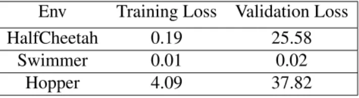
Table 3.1: Comparison between training loss and validation loss in various environments. Training loss is smaller than the validation loss, indicating an overfitting of the neural network model to the training data.

Env Training Loss Validation Loss HalfCheetah 0.19 25.58

Swimmer 0.01 0.02 Hopper 4.09 37.82

3.3

Building an Accurate Model

From above experiments, we can see that the model could be quite accurate for input from the same distribution (training data), but the problem is that it cannot handle well the input data from a different distribution (validation data). We can interpret the problem as the generalization problem in deep learning, where neural network overfits to the training data. We propose two future direction to alleviate the problem.

3.3.1

Exploration

One way to build a more accurate model is to leverage exploration policy and methodology to collect more diverse data. Diverse data means that the training input could cover the entire input state-action space. Combining the more accurate model with model-based decision making, we aim to achieve a better performance.

The problem that exploration tries to solve could be illustrated from another perspective. Currently model-based algorithm often converges to a sub-optimal performance, which is a

(22)

local minima. It’s reported that algorithms with learned dynamics are stuck at performance local minima significantly worse than using ground-truth dynamics [WBC+19a]. We propose that exploration would be an effective strategy to improve model learning. While exploration and off-policy learning have been studied, it has been barely addressed on current model-based approaches [WBC+19b].

An inaccurate model caused by poor exploration would lead to a suboptimal performance. Model-based controller or policy would guide model learning. For instance, in PETS algorithm [CCML18], the data used to learn model is collected from the MPC controller’s data and model learned would overfit to those data, since it doesn’t validate the learned model using unseen data. The policy deployed would be only locally optimal with respective to the model, so that the performance can only reach to a local optima. Second, [KCD+18] reported that the learned policy tends to exploit regions where insufficient data is available for the model to be learned, i.e it utilizes the trajectory that the learned model predict incorrectly compared to the ground truth dynamics. The policy optimization stage after model learning stage would steer the optimization towards areas where the model is inaccurate. It would be better to learn a globally correct model via thorough exploration i.e. be as close as possible to the ground truth dynamics, then planning on the globally correct model would lead to better performance. Once we get a globally accurate model, with a good policy training algorithm, the policy would be globally optimal and not exploit inaccurate regions.

Back to the observation that the neural network overfits to the training data, we can infer that if we have a meaningful dataset from environment - a dataset that is diverse enough to cover the entire state-action space, the problem of overfitting could be solved, since it could cover the validation input space. A promising direction is to use exploration strategies to help the agent visit more diverse input space. Then we can learn a globally accurate dynamics model.

Experiments DesignWe plan to use samples collected by an exploration policy to train a model and compare the performance of the model with the performance of baseline model trained

(23)

by samples from non-exploration policy (pretrained TRPO policy or random policy). We train another TRPO policy by collecting fictitious samples from the model, i.e fitting a TRPO policy to the learned model. The performance of the model is evaluated by the return of the TRPO policy in real environment. The main difference between the model with exploration and baseline model is that exploration policy could collect more diverse data, whereas non-exploration policy like pretrained TRPO policy or random policy would just exploit a limited subset of entire state space.

3.3.2

Adaptation

Besides exploration strategy, we can use adaptation methods to solve the problem that how to generalize the model to make an accurate prediction given input from distribution different from the training distribution. Learning dynamics model that can be adapted online fast to deal with unseen situation is the promising direction.

Learning to adapt to unseen dynamics is the way that we believe to solve model learning problem - overfitting to the training data. We should first meta-train the model parameters. When facing unseen input, the meta parameter could then be updated quickly in few gradient steps to fit the current dynamics. Then the updated model could be used to do planning.

3.4

Model Learning and Policy Optimization

Model learning and decision making could not be separated in model-based reinforcement learning methods. In this section, we focus on the role of model learning in policy optimization. Specifically we use model-based RL algorithm ME-TRPO and MBPO to evaluate the model learning process and the role of its policy optimization part. The benchmark we use for the following experiments is HalfCheetah environment in Mujoco.

ME-TRPO is a vanilla model-based reinforcement learning algorithm, which uses TRPO to optimize the policy on an ensemble of models. Original paper shows its lower sample

(24)

com-plexity compared to model-free deep RL methods on challenging continuous control benchmark tasks. We show the algorithm of ME-TRPO here in Algorithm 1. The algorithm iteratively does two steps. First, use the policy to gather data to train a model dynamics on it. Second, optimize the policy using TRPO on the learned dynamics instead of the real environment.

Algorithm 1Model-Ensemble Trust Region Policy Optimization (ME-TRPO)

1: Initialize model network parameters and policyπθ

2: Initialize an empty dataset

D

3: fornouter iterationsdo

4: Collect samples from the real environment usingπθadd them to

D

5: Train all models using

D

6: fornpolicy iterationsdo

7: Collect fictitous samples from the learned model usingπθ

8: Optimize the policy using TRPO on the fictitious samples

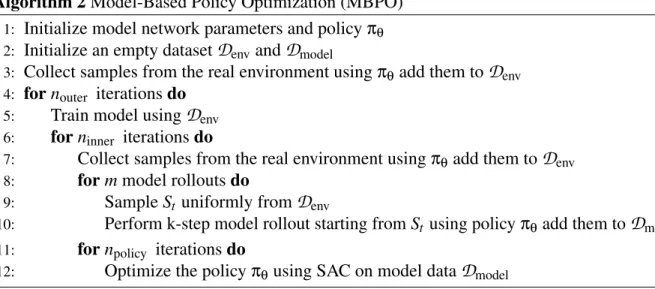
We also uses the algorithm MBPO (shown in Algorithm 2) to evaluate the model-based learning and policy optimization. MBPO utilizes short model-generated rollouts instead of generating rollouts from the initial state distribution. As we mentioned earlier in Chapter 2, multi-step prediction on an inaccurate model would cause compounding error. The intuition to reduce compounding error is to avoid using long rollouts by using branching strategy to generate short rollouts. Branching strategy in MBPO which model rollouts begin from the state distribution of a different policy under the true environment dynamics effectively relieves the compounding model error problem caused by long rollouts generated from inaccurate models. In practice, branching replaces few long rollouts from the initial state distribution with many short rollouts starting from replay buffer states.

In reinforcement learning setting, the overall objective is to minimize the cumulative cost (or maximize the cumulative reward). At each iteration, ME-TRPO learns the model first and fit a policy on the model. We validate the policy using the model to get the model cost and using the real world to get the true cost. The performance on the model and real world are shown in Figure 3.1. It appears that the policy fitting to the learned model always performs better in the learned

(25)

Algorithm 2Model-Based Policy Optimization (MBPO)

1: Initialize model network parameters and policyπθ

2: Initialize an empty dataset

Denv

and

Dmodel

Denv

4: fornouter iterationsdo

5: Train model using

Denv

6: forn_inner iterationsdo

D

env

8: formmodel rolloutsdo

9: SampleS_t uniformly from

Denv

10: Perform k-step model rollout starting fromS_t using policyπθadd them to

Dmodel

11: forn_policy iterationsdo

12: Optimize the policyπθusing SAC on model data

Dmodel

model than in the real world, indicating the model bias compared to true dynamics. Also, as the training steps go up, the learned model performs better in the real world. To seek why, we plot the dynamics validation loss to show how accurate the model is.

Figure 3.1: Comparison between real cost and model cost in ME-TRPO. The policy fitting to the learned model always performs better in the learned model than in the real world, indicating the model bias compared to true dynamics

Plotting the dynamics model validation loss in Figure 3.2, We see learning a more accurate model would improve the policy performance in real world. As more (probably better) data are collected by the updated policy, dynamics validation loss becomes lower, which means the model

(26)

Figure 3.2: Dynamics validation loss in ME-TRPO. Dynamics validation loss decreases as the training steps goes up.

is less overfitted. The more accurate dynamics model corresponds to the improved performance in real world in Figure 3.1. As the agent learns a more accurate model, the performance in real world goes up. Note that the dynamics model training loss is always below 1 indicated in Table 3.1, and dynamics validation loss is much higher than 1 in Figure 3.2, which means that model significantly overfits to the training data.

Training Data vs Model LossIn order to understand how to learn an accurate model, an interesting direction is to investigate how more data could lower the validation loss. We can see from Figure 3.2 that more data collected from the updated policies could lower the validation loss. To see how data size would affect validation loss, we use a random policy to collect additional data. To be more specific, we directly use a random policy to sample a dataset of 63000 timesteps. The result is that the loss could converge to 5, which is much lower than the lowest value 20 in Figure 3.2. This indicates that more data could lower the validation loss. We only know that more data could lower the loss but we are still not sure how more data could lower the validation loss.

As we can see from the Figure 3.2 and Figure 3.1, the model loss is always decreasing, but the policy performance stops increasing after 60000 steps. Policy performance converges but

(27)

the model loss does not. This interesting observation could help explain how the model loss is lowered as more data is collected. It indicates that a lower model loss could be simply caused by more training data (collected from a similar policy) rather than more better training data (collected from an updated policy).

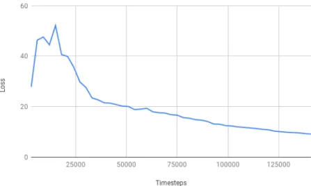
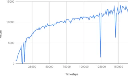
Figure 3.3: MBPO’s learning curve on HalfCheetah environment.

Figure 3.4: MBPO Dynamics validation loss.

Model Loss vs Policy Performance Although experiment result from ME-TRPO and MBPO Figure 3.2 and 3.1 indicates a relationship between validation loss and average cost.

(28)

However, we don’t think a lower validation loss could directly lead to better average cost. A small validation loss means that the model is accurate in the test region, but a small validation loss might not help to learn a good policy to achieve low average cost, since the test region might not be used by the policy to achieve a good average cost. In contrast, the policy might utilize other regions outside the test regions, where the model is inaccurate. In other words, the average cost performance might depend on the regions outside the training and test dataset. Policy might exploit the region where the data is scarce (thus inaccurate region) to get a bad cost. Thus a lower validation loss might not lead to better average cost.

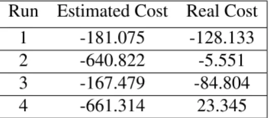
Table 3.2: Performance of TRPO on model trained from 63000 randomly collected data in several runs. These three runs are all initialized with 63000 randomly collected data. The result indicates the ME-TRPO’s performance is not stable when using randomly collected data.

Run Estimated Cost Real Cost 1 -181.075 -128.133 2 -640.822 -5.551 3 -167.479 -84.804 4 -661.314 23.345

We then evaluate the performance of TRPO on the model trained from 63000 randomly collected data. We use TRPO algorithm to train a policy in the learned model. Estimated validation cost could achieve -181 and real validation cost could achieve -128. However, after several different runs, we found out that the result is not stable and the difference between real validation cost and estimated validation cost could be very high. Table 3.2 shows the performance from several runs. This indicates that although the model is accurate on its training data and test data, but it is not globally correct and cannot generalize to other region which the policy exploits. We attribute instability to the reason that the random policy collects different kind of data and introduces great amount of stochasticity to the result. This also demonstrates that random exploration is not sufficient to collect data for learning a useful model, whereas an iterative process of alternatively improving the model and policy utilized by ME-TRPO could result a

(29)

good performance. In the future, we want to find the underlying factor that would be influenced by the validation loss and could improve the average cost.

Simply using a random policy to collect data doesn’t help to build a model that is useful for learning a practical policy. It shows that collecting data to learn model is an exploration problem. This fact also indicates that ME-TRPO works well by simultaneously update the policy and model. Learned model could be improved by data collected from policy, and policy is updated by imagined trajectories from the new model. Using the updated policy to collect data is a better method to explore the dynamics than the old policy. This way could build a model whose accurate region could be exploited by the policy. Then the data collected by the updated policy is its local data with lower cost, which helps to train a better local model with lower loss. We also include MBPO’s policy and model learning curve to emphasize the observation that the model and policy simultaneously improve in Figure 3.3 and Figure 3.4.

(30)

Chapter 4

Safe Reinforcement Learning

4.1

Introduction

Safety is an important issue in Artificial Intelligence. One topic in AI safety is the safe exploration for reinforcement learning, in which we want to prevent the learning agent doing bad actions that could lead to disastrous outcomes. In other words, the agent needs to learn a safe policy that would satisfy some constraints, such as avoiding obstacles in the environment. Thus, safe RL has become an important topic among artificial intelligence researchers.

In the chapter, we want to tackle the problem of safe reinforcement learning by incorpo-rating the idea of model-based reinforcement learning.

Many approaches have been developed for safe RL. They fall into two categories, based on whether the goal is to achieve constraint-conforming behaviors asymptotically or throughout the learning process. To achieve asymptotic safety, since the problem of RL is about maximizing a numerical reward signal [SB98], safe RL can be considered as a constrained optimization problem. Various modifications to policy gradient methods can be used. Constrained update approaches extend policy optimization algorithms to constrained optimization; for example, constrained policy optimization (CPO) [AHTA17] uses a trust region approach originated from the numerical

(31)

optimization community. CPO proposes a search algorithm for constrained reinforcement learning with guarantees for near-constraint satisfaction at each iteration. The problem of near-zero violation throughout the training process is a much harder problem, and it is typically assumed that very strong supervision has to be provided to ensure a safe learning process. Existing approaches have assumed the use of pre-trained safe backup policies [HSSU08], pre-designed safe controllers [PB03], or pre-defined Lyapunov functions [BTSK17] or control barrier functions [COMB19] that can avoid exerting unsafe actions at every step of training. The problem of training safe RL with near-zero violation during the training process without access to external oracles remains largely open.

We propose a new approach for safe reinforcement learning that leverages model-based methods to ensure near-zero violation throughout the training process and without using external guidance such as pretrained safe policies or control barrier functions. We observe that humans and animals learn safe behaviors always through multiple steps or learning stages. While most of us learned how to driving without ever crashing a car, no one learns the skill by learning to drive from scratch on a busy road. We start with driving in an open space to gradually understand the effects of our actions in the state of the vehicles. We then learn to handle constraints, i.e. avoiding obstacles, in controlled environments. When we have learned both how to get to a destination in open space, and how to avoid obstacles in a controlled space, we can drive in real traffic and fairly quickly learn how to drive safely to a destination in a variety of road conditions. This three step learning process occur naturally in the process of acquiring any advanced skill. Our goal in this paper is to formally design a similar framework for artificial agents that tightly integrates various state-of-the-art methods in policy optimization, model-based reinforcement learning, imitation learning, hierarchical reinforcement learning and curriculum learning.

We propose a three-step curriculum to achieve safe learning. First, we train the agent in a constraint-free environment to learn a normal policy for achieving high rewards, and a dynamics model at the same time. Second, utilizing the dynamics model, we use model-based method to

(32)

train the agent in a constrained environment to learn how to avoid violating safety constraints without aiming to achieve its goals in the first step. Finally, we train the agent in a constraint environment to learn a hierarchical policy that can choose between the two types of policies to both achieve goals and avoid unsafe behaviors. One important assumption behind the curriculum is that there should be no change in dynamics for all the time. Thus in the second and third steps, the agent exploits the dynamics model learned from the first step to perform model-based learning, and use imitation learning to formulate a global policy. Breaking the learning task down to these multiple stages show significant benefits both in terms of performance, safety, and overall sample complexity and performance. Throughout the training process, we ensure near-zero violation of the safety properties, and the agent does not have access to pre-trained safe policies or external guidance such as barrier functions.

Model-based methods allow the agent to gain knowledge about the environment and to predict the consequences of actions before they are taken, allowing the agent to generate virtual experience. In other words, the intuition is that if the agent knows the dynamics well, it could avoid obstacles in the environment by doing model-based planning. The intuition of the model-based safe policy part is from how we learn in our daily-life. For instance, Learn how to surf. When we are learn surfing, we would start with learning paddle in still water like swimming pool. After getting familiar with the environment, we then switch to the more advanced area with small waves. This could reduce the risk to some extent compared to directly jumping into waves without any practice in still water.

There were few safe exploration work using model-based methods in that model-based method cannot be used in large space and stochastic problems in which the approximation of an accurate model from which derive a good policy is not possible. Building models have been an open issue and key ingredient of research and progress in the field. Thanks to the development of deep learning, the dynamic model could be represented by the neural network which can handle complex state space, so using model-based method in safe exploration becomes possible.

(33)

Connected to model learning problems in previous chapters, an aggressive exploration policy in order to build an accurate model would still lead to catastrophic consequence, thus making model-based approaches suffer a similar exploration problem as model-free approaches. So the question is: how can we safely explore the relevant parts of the state/action spaces to build up a sufficiently accurate dynamics model from which derive a good policy? Abbeel (2008) offers a solution to these problems by learning a dynamics model from teacher demonstrations. Our method offers another solution by first training the neural networks model in a simpler, constraint-free environment and then leverage the learned dynamics in a more complex, dangerous environment. The model-based RL algorithm could guarantee to work well because, given an accurate dynamics, model predictive control (MPC) would not select the low-reward action, thus not violating the constraint and achieving safe exploration. From another perspective, we are actually using model-based method to do transfer learning, transferring the knowledge about the environment from one task to another task, with a goal to keep the exploration process safe.

In the last step, we learn a hierarchical policy that can choose between the two types of policies to both achieve goals (constrained-free) and avoid unsafe behaviors (model-based). Here constrained-free method can be regular model-free RL algorithms. As there is a trade-off between model-based and model-free algorithm, model-based methods have relative higher computational complexity and lower sample complexity than model-free methods. We believe a combination of model-based and model-free methods would be a better strategy to tackle RL problem than any single of them. In our problem setting, model-based method, regarded as an ”expert” policy, could be used to guide the agent in the region where there are constraints or obstacles, while model-free policy could be used for safe regions with no constraints and obstacles. Thus we can efficiently leverage the advantage of model-based and model-free methods.

This chapter is organized as follows. After reviewing related work in Section 4.2, we describe the three-step curriculum for safe learning in Section 4.3. We evaluate the performance of the proposed algorithm on complex constrained tasks such as Mujuco Ant and Pybullet Racecar

(34)

in Section 4.4. We demonstrate the clear benefits of the proposed methods in comparison with state-of-the-art methods such as Constrained Policy Optimization.

4.2

Related Work

Safe RL has been extensively studied under different formalisms [GF15]. One common framework incorporates constraints into sequential decision making problems using Constrained Markov Decision Process (CMDP) [Alt99]. A CMDP is an MDP with additional cost signals for each state-action pair. The objective remains the same as maximizing the cumulative reward (the expected return) but now it is subject to the constraints that cumulative costs are below their respective thresholds. Note that constraints in CMDPs define probabilistic properties and model sequential decision problems with constraints to be conformed asymptotically. Many recent methods are based on the CMDP framework. CPO [AHTA17] is a practical policy optimization algorithm for CMDPs that approximately guarantees monotonic improvement on expected return together with constraint satisfaction at each iteration using a trust region approach. Reward Constraint Policy Optimization [TMM19] proposes multi-timescale algorithms that optimize over a reformulated unconstrained optimization problem, with penalties for constraint violations added to the objective function using Lagrange relaxation. A constrained cross-entropy method for CMDPs is presented in [WT18], in which sampled policies are sorted based on how well the constraints are satisfied. [CNDGG18] and [CNF+19] propose methods for finding Lyapunov functions that can enforce constraints in CMDPs, so that safe policies with upper-bounded expected constraint costs can be learned using dynamic programming and policy gradient in discrete and continuous action spaces.

On the other hand, various existing approaches have focused on ensuring safety throughout the entire learning process. [DDV+18] extends [PDMT18] and formally defines state-wise constrained MDPs. It uses a pre-trained linear approximation of the dynamics to set up a safety

(35)

monitor on top of learned policies, and this guarantees zero violation of state-wise hard constraints. The proposed approach enforces a strong assumption that a single safe action is always strong enough to direct the agent away from any potentially unsafe behavior. [BTSK17] uses predefined Lyapunov functions to stabilize an AI controller allowing safe explorations that provide the basis for improvements on policies. [PB03] makes of Lyapunov functions to prepare pre-designed safe control laws for RL agents to choose from. Artificial potential fields popularly used in robotics [Kha85] have also been linked to safe RL [XWZL16]. [COMB19] proposes a controller synthesis algorithm that uses control barrier functions to guide a model-free RL controller at every training step to improve exploration and guarantee safety.

A curriculum generation method has been proposed in [EGIL18]. The approach uses a forward and a reset policy that are learned concurrently, resetting the environment before entering an non-reversible state. [GF12] improves a safe but suboptimal policy using techniques such as case-based reasoning. Backup policies are employed in [HSSU08]. Safe exploration in ergodic MDPs and finite MDPs is studied in [MA12] and [TBK16], respectively. Off-policy evaluation for safe RL is investigated in [Tho15]. [BJ10] and [CGJP17] study risk-constrained MDPs with constraints on conditional value-at-risk, with the latter proposing a policy gradient-based approach combined with the Lagrangian method. [SSSE18] presents a human-in-the-loop framework where a human can always substitute an unsafe action with a safe one.

4.3

Problem Formulation

Markov Decision Processes (MDPs) provide a mathematical formalism for RL. An MDP consists of a set of states

S

, a set of actions

A

, a transition modelP(s0|s,a)denoting the probability of reaching states0∈

S

by taking actiona∈

A

in states∈

S

, and a reward signalR(s,a)describing the reward for a state-action pair (s,a). In RL, the goal of an agent is to learn a deterministic or stochastic policyπ(a|s)to maximize the cumulative reward. More formally, the goal is to

(36)

find π∗=argmax_π_∈_Π J(π)whereJ(π) =_Eπ[∑_t∞₌₀γtR(st,at)]and γ∈[0,1]is a discount factor

[SB98, RN09].

We focus on the problem safe RL for MDPs with constraints satisfied throughout the learning process. The mathematical formalism we use is similar to the state-wise constrained MDPs in [DDV+18]. We introduce the hard-constrained Markov decision processes (HCMDPs). In an HCMDP, an agent is constrained to always stay in a set of safe states. Formally, let

Ssafe

⊆

S

be the set of safe states, an HCMDP is a MDP with the constraints_t∈S_safeat each time stampt. Then the RL problem in a finite-horizon HCMDP is argmax_θsuch thats_t∈

Ssafe

for allt∈[T], whereJ(πθ) =Eπ[∑∞t=0γtR(st,at)].

We consider robot locomotion tasks [TET12, BCP+16], such as the ones shown in Figure 4.2. The underlying transition model in these RL problems [FGKM18] can be represented in the form of a dynamical system (either stochastic or deterministic). Model-based RL (MBRL) studies how to learn dynamics models that many classic algorithms in planning and control can use. Model-based RL algorithms typically enjoy low sample complexity in comparison with model-free methods: With a learned dynamics model, the required number of interactions with the environment can be significantly reduced [WBC+19b]. Model-based approaches therefore have an edge on safety-critical control tasks, as fewer interactions can mean fewer chances to take an unsafe action.

4.4

Curriculum for Safe Learning

We propose a three-stage learning process to achieve safe RL without relying on any pre-trained safe policies or oracle guidance. Algorithm 3 shows the overall procedure.

(37)

Algorithm 3A high-level scheme of our proposed model-based curriculum for safe RL.

1: Step I: Constraint-Free Learning

2: Use SAC to train a performant policy πfree while collecting data D={(s,a,s0)} for all

timesteps

3: Learn dynamics model ˆf(s,a)on mini-batches of dataDby minimizing 1_u∑ui=1(fˆ(s,a)−s0)2.

4: Step II: Learning Safeguarding Policies

5: D=0/

6: forv=0 to number of roundsT_N do

7: Initializes_t←s

8: forw=0 to number of steps per roundTL do

9: Sample and rankNtrajectoriesτj(st) ={stj+i} k−1

i=0,∀j∈N

10: Chooseτ∗(st)that maximizes the cumulative reward

11: Execute the first actiona_t∗

12: s_t ←s_t∗₊₁

13: D←D∩(st,a∗t).

14: Learn safeguarding policyπsafewithDthrough imitation.

15: Step III: Mixing Safe and Performant Policies

16: D=0/

17: forv=0 to number of roundsTN do

18: Initializes_t←s

19: forw=0 to number of steps per roundT_L do

20: Sample choicem∼ {FREE,SAFE}, based on which sample actionsa∼πm(st)

21: Sample and rank M trajectoriesτj(st) ={s_tj₊_i} k−1

i=0,∀j∈M

22: Chooseτ∗(st)that maximizes the cumulative reward

23: Obtain choice sequence{m∗_t₊_i}k_i₌−1₀ that producedτ∗(st)

24: Execute the first actiona_t∗

25: D←D∩(st,m∗t).

(38)

4.4.1

Step I: Constraint-Free Learning

In the first step of the curriculum, the agent learns in a constraint-free environment. This enables the agent to learn a constraint-free performant policy that maximizes reward signals such as reaching goals in the space. At the same time, the agent learns a dynamics model of the environment, i.e., how state-action pairs are mapped to the next states.

In this step, we use soft actor-critic (SAC) [HZAL18] for learning the performant policy. SAC is a model-free deep RL algorithm with state-of-the-art performance on a variety of standard continuous control tasks. SAC incorporates the expected entropy of a policy into the objective function to encourage exploration, by maximizing_Eπ[∑∞_t₌₀γt(R(st,at) +H(π(·|st)))]whereHis

the entropy of a policy. The entropy term provides extra exploration that produces more diverse samples of the environment dynamics, but other popular training methods such as [SLA+15, SWD+17b] can also be used for generating the experiences. We collect transition tuplesD=

{(s,a,s0)}for learning the dynamics. We then use a neural network model to learn the dynamics

through standard mini-batch learning by minimizing 1_u∑ui=1(sˆi−si)2, where ˆsis the next state

generated by our candidate dynamics with minibatches of sizeu.

4.4.2

Step II: Learning Safeguarding Policies

In the second step of the curriculum, the agent learns a safeguarding policy with respect to constraints. While previous work (CPO) uses a cost function in addition to the reward function to represent the constraint, we shape the reward function to represent the constraint. The reward function now only encodes the constraints, so the objective of the agent is only to avoid unsafe regions without trying to achieve other goals.

To define the reward functions for this step, we introduce artificial potential fields as commonly used in robotics [Kha85]. We design reward signals that form a scalar field around the unsafe areas and can indicate whether an agent is getting close to unsafety. For example,

(39)

we typically define the reward function to beR(s) =−c·x−2, wherexrepresents the minimum distance from a statesto the unsafe area. This reward function provides a buffer area that allows the agent to sample several actions without entering the unsafe area.

Now, using the learned approximate dynamics model from Step I, the agent can use rewards provided by the potential field to tell the difference between safe and unsafe action sequences. We use model predictive control (MPC) [GPM89] to plan the actions. Specifically, at each states_t, we sampleNsequences ofkactions{a_ti,a_ti₊₁, . . . ,a_ti₊_k₋₁}N

i=1and use our learned

dynamics ˆf to predict what states{sî_t₊₁,sî_t₊₂, . . . ,sî_t₊_k}N

i=1will be visited. The actions are only

simulated and not actually taken in the environment. We then pick the most promising trajectory based on cumulative rewards ∑k_i=1R(st+i,at+i)and execute the first action. In addition, if the

agent can sample a trajectory that ensures safety according to the dynamics model, then it can directly execute all actions in the sampled sequence. Lines 5 to 13 in Algorithm 3 show this procedure. This model-based approach ensures low sample complexity for learning the safeguarding policy (Section 4.5.2).

To form a safeguarding policy, we treat the actions that are taken by the agent as expert actions, and use a deep neural network policy to imitate them. For imitation, we use the sample-efficient Dataset Aggregation (DAgger) [RGB11] algorithm that allows the agent to learn interactively from the expert.

By the end of Step II, the agent has learned a safeguarding policy πsafe with near-zero

violation of the safety properties, as confirmed by experiments shown in Section 5.

The model-based approach for learning the safeguarding policy has advantages both in terms of safety and sample complexity. On one hand, an agent does not need to physically move but can instead plan and predict what state it will be in by taking an action. On the other hand, in most cases, we resample new trajectories after an agent executes an action. This minimizes the effects potentially caused by errors in learned dynamics, and therefore makes our approach more robust.

(40)

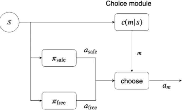
Figure 4.1: Mixing safe and performant policy

4.4.3

Step III: Mixing Safe and Performant Policies

After the previous two steps of training, the agent has learned a performant policy that optimizes its action for achieving goals, and also a safeguarding policy for avoiding unsafe behaviors. In this third step of training, the agent only needs to learn when to invoke which of these two types of policies. The action space now is simply the choice between the policies, and we can use the same model-based learning techniques as Step II to efficiently learn. The difference is now the overall policy needs a hierarchical structure that properly mixes the performant and safe policies, which we design as follows.

The mixture policy consists of two modules, a choice module and a control module. The choice module outputs a distribution over the sub-control policies (the safe one and the performant one). Figure 4.1 shows the architecture. For each states, the agent first use the choice module to obtain the distribution of its choices, i.e.,P(c_i|s)for each choicec_i. It then uses the policyπithat

corresponds to the the highest ranked choice to sample the action. Thus, the overall distribution can be represented in the the following factored form:

πθ(a|s) =

∑

i∈C

c_θ(i|s)πi,θ(a|s) (4.1)

(41)

second steps of training. The reward function now is simply a weighted sum of the ones from Step I and Step II, and the agent can learn quickly under this weak signal (see Section 4.5).

4.5

Experiments

We perform experiments on three constrained environments in OpenAI Gym, Mujoco and PyBullet. Figure 4.2 shows an overview of the environments. We first show that the proposed methods allow the agents to achieve goals without violating safety properties during training. Second, we compare with constrained policy optimization methods (CPO) and show benefits both in safety and in performance. In the end, we perform ablation study to show that the separation of different stages in the training process is crucial for the success of the approach.

(a) (b) (c)

Figure 4.2: Three constrained environments. Left: Reacher with vertical barrier. Middle: Racecar with three random red boxes as obstacles and one ball indicating the destination. Right: Ant with two parallel barriers with red lines and two parallel buffer areas with blue lines. The agent violates safety when it hits any obstacle or barrier.

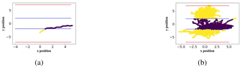
(a) (b)

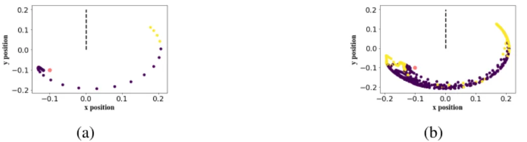
Figure 4.3: Sample trajectories for the Reacher environment (Figure 4.2a). The yellow points are the choice of safe policy and the brown points are the choice of free policy. The top dotted line is the constraint, the red point is the random target. (a) One trajectory of the agent. (b) A large subset of trajectories of the agent.

(42)

4.5.1

Environments

Reacher. We perform experiment in Mujuco Reacher, adding the constraint that the agent can never touch the vertical bar (Figure 4.2a). Figure 4.3 shows some trajectories of Reacher during Step III of the curriculum. Figure 4.3a shows one sample trajectory during training. The fingerpoint of Reacher is close to the barrier at first. It then becomes aware of the danger and chooses the safeguarding policy by moving down the arm to avoid the barrier. When being far away from the obstacle, it chooses the constraint-free policy to reach the target. Figure 4.3b shows all sampled actions in the training process with the consistent behavior of making the right choices between the two policies.

(a) (b)

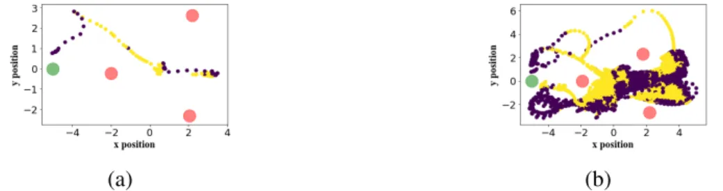
Figure 4.4: Sample trajectories for the Racecar environment (Figure 4.2b). The three red points are the random obstacles. The blue point is the destination. The yellow point means the agent chooses the safe policy at the current state, whereas the brown point means the free policy. (a) One trajectory of the agent. (b) A large subset of trajectories of the agent.

Racecar. We evaluated our algorithm on Racecar in the Pybullet environment with random obstacles and a destination. The goal is to reach the destination and always avoid obstacles. Figure 4.4 shows trajectories of Racecar during training in Step III. When the agent is close to the obstacle, it would choose the safe policy to avoid hitting the obstacle. When being away from the obstacles, it would choose the free policy to reach the destination. Figure 5b shows all the trajectories during training, and it is clear that the agent would select safe policy near the obstacles.

(43)

(a) (b)

Figure 4.5: Sample trajectories for the Ant environment (Figure 4.2c). The area between the blue line and the red line is the buffer area. The red lines are parallel barriers. Outside the red lines is the violation area. (a) One trajectory of the agent. (b) A large subset of trajectories of the agent.

Ant. We perform experiments in the Mujoco Ant environment with parallel barriers and buffers, which is the same setting as [AHTA17] (Figure 4.2c). The two red lines are the barriers and the areas between red lines and blue lines are the buffer areas. The ant needs to move forward while avoiding the two-sided barriers. Figure 4.5a shows one trajectory of the agent during training. When the agent is in the dangerous buffer area, it would walk back to the safe area to avoid the barriers. When the agent is in the safe area, it uses the performant policy to walk ahead. Figure 4.5b shows all trajectories and the agent can clearly choose correctly between safe and performant policies.

4.5.2

Comparison with Baseline

We compare the proposed methods with state-of-the-art safe learning algorithm CPO [AHTA17]. The two methods can be compared directly, because in both algorithms the agent learns only using fixed reward function from the environment without access to pre-trained safe policies, analytical control solutions, or barrier functions. Since it has already been shown that CPO significantly outperforms other model-free methods in terms of enforcing constraints, we focus on the comparison with CPO.

In Figure 4.6, we show the overall learning curve and the number of constraint violation throughout the training process. As Figure 4.6b, Figure 4.6d and Figure 4.6f show, the agent

(44)

(a) (b)

(c) (d)

(e) (f)

Figure 4.6: Compares rewards and violations with CPO in Reacher, Racecar and Ant.

trained in our curriculum always achieves near-zero violation, while CPO can often achieve the same behavior eventually, but not during training. CPO violates the constraint for many times during training. In terms of learning performance, the reward functions measures the weighted sum of getting to the goal and penalty of constraint violation, and the optimal performance should achieve values close to zero. In Figure 4.6, we observe the trend of CPO in terms of gradually achieving higher performance. CPO gets very low reward at the initial phase of training process, so in these figures, the rewards of our methods can appear flat. We show a closer view of our learning curves in Figure 4.7.

Moreover, Figure 4.8 shows the comparison with CPO in terms of sample complexity. The most costly part of our curriculum is the first step of constraint-free learning, which uses model-free methods but can be changed to more sample-efficient ones too. In Step II and III, the safe learning procedures use model-based learning and imitation learning, and are very sample

(45)

efficient. This suggests that the procedures can potentially be used in real robots to perform online safe learning, using dynamics models learned offline through simulation.

(a) (b)

Figure 4.7: The true rewards in our algorithm. (a) is the reward of Racecar. (b) is the reward of Reacher.

Figure 4.8: Complexity of racecar, reacher and ant in our curriculum.

4.5.3

Importance of Curriculum Learning

To see the importance of the three-step curriculum, we further compare with results using a simpler design. In Figure 4.9a, we show quick violation of safety, when we directly combine both the goal-achieving and safety-penalty rewards in Step II. Figure 4.9c and Figure 4.9d show the learning curves in this setting. In Figure 4.9e and 4.9f, we use PPO-training instead of model-based to learn the switching between two pretrained safe and performant policies. The performance is much worse than the model-based curriculum. Figure 4.9b shows a trajectory from the PPO-trained mixture policy, which indicates a violation of safety.

(46)

(a) (b)

(c) (d)

(e) (f)

Figure 4.9: Ablation Study. (a) and (b) illustrate the violation situation in ablation study. (c) and (d) illustrate learning using Step II alone. (e) and (f) illustrate using PPO training instead of model-based learning.

with Yixuan Huang, Zhi Wang, Yuda Song and Sicun Gao. The thesis author was a co-author of this material.

(47)

Chapter 5

Conclusion

In the model learning chapter, we analyze the popular model-based reinforcement learning algorithms and try to understand it through novel experiments. We put more emphasis on the model learning part of the algorithm and evaluate the role of the model learning in policy optimization. An important point that we confirmed is that model should be optimized to fit the policy and policy should be optimized to fit the model simultaneously. We also proposed method to learn a global accurate model through exploration strategy to visit diverse space. Also, meta learning could be used on model learning part, where model is trained to adapt to the new input. In the safe learning chapter, we propose a three-step model-based curriculum for solving safe RL problems, inspired by how humans learn to perform safe actions. Such a curriculum separates the training of two policies, one for reward maximization and the other constraint satisfaction, and employs a factored structure that properly mixes the two policies. Our curriculum ensures near-zero violation of safety constraints throughout the entire learning process by also incorporating techniques such as potential functions and model predictive control. On a variety of continuous control tasks, we also showed empirically that our approach had better performance in terms of constraint satisfaction and better sample complexity in comparison with CPO, a state-of-the-art policy gradient algorithm. The low sample complexity potentially enables our

(48)

curriculum to be applied online. For future work, we believe it is promising to use the proposed methods in real-world physical environments, and use offline-trained performant and models to achieve safe reinforcement learning online. It is also promising to further improve performance when stronger guidance can be given.

How to properly combine the first step and second step in curriculum learning would be a research question. In order to select between the model-based policy and model-free policy, our idea is to construct a switch policy. We show that using model predictive control on mixture policy would work well, but there might be better methods to choose between the constraint-free policy and safeguarding policy. How to learn this kind of switch policy would be a promising future direction.

(49)

Bibliography

[AHTA17] Joshua Achiam, David Held, Aviv Tamar, and Pieter Abbeel. Constrained policy optimization. InProceedings of the 34th International Conference on Machine Learning (ICML), volume 70, pages 22–31, 2017.

[Alt99] Eitan Altman. Constrained Markov decision processes, volume 7. CRC Press, 1999.

[BCP+16] Greg Brockman, Vicki Cheung, Ludwig Pettersson, Jonas Schneider, John Schul-man, Jie Tang, and Wojciech Zaremba. Openai gym. CoRR, abs/1606.01540, 2016.

[BHT+18] Jacob Buckman, Danijar Hafner, George Tucker, Eugene Brevdo, and Honglak Lee. Sample-efficient reinforcement learning with stochastic ensemble value expansion. InAdvances in Neural Information Processing Systems, pages 8224– 8234, 2018.

[BJ10] Vivek Borkar and Rahul Jain. Risk-constrained markov decision processes. In

49th IEEE Conference on Decision and Control (CDC), pages 2664–2669. IEEE, 2010.

[BTSK17] Felix Berkenkamp, Matteo Turchetta, Angela P. Schoellig, and Andreas Krause. Safe model-based reinforcement learning with stability guarantees. In Proceed-ings of the 31st International Conference on Neural Information Processing Systems (NeurIPS), pages 908–919, 2017.

[CCML18] Kurtland Chua, Roberto Calandra, Rowan McAllister, and Sergey Levine. Deep reinforcement learning in a handful of trials using probabilistic dynamics models. InAdvances in Neural Information Processing Systems, pages 4754–4765, 2018.

[CGJP17] Yinlam Chow, Mohammad Ghavamzadeh, Lucas Janson, and Marco Pavone. Risk-constrained reinforcement learning with percentile risk criteria.The Journal of Machine Learning Research, 18(1):6070–6120, 2017.

(50)

[CNDGG18] Yinlam Chow, Ofir Nachum, Edgar Duenez-Guzman, and Mohammad Ghavamzadeh. A lyapunov-based approach to safe reinforcement learning. In Pro-ceedings of the 32nd International Conference on Neural Information Processing Systems (NeurIPS), pages 8103–8112, 2018.

[CNF+19] Yinlam Chow, Ofir Nachum, Aleksandra Faust, Mohammad Ghavamzadeh, and Edgar Duenez-Guzman. Lyapunov-based safe policy optimization for continuous control. InReinforcement Learning for Real Life (RL4RealLife) Workshop in the 36th ICML, 2019.

[COMB19] Richard Cheng, G´abor Orosz, Richard M. Murray, and Joel W. Burdick. End-to-end safe reinforcement learning through barrier functions for safety-critical continuous control tasks. InThe 33rd AAAI Conference on Artificial Intelligence, pages 3387–3395, 2019.

[CRS+18] Ignasi Clavera, Jonas Rothfuss, John Schulman, Yasuhiro Fujita, Tamim As-four, and Pieter Abbeel. Model-based reinforcement learning via meta-policy optimization. arXiv preprint arXiv:1809.05214, 2018.

[DDV+18] Gal Dalal, Krishnamurthy Dvijotham, Matej Vecerik, Todd Hester, Cosmin Paduraru, and Yuval Tassa. Safe exploration in continuous action spaces. arXiv preprint arXiv:1801.08757, 2018.

[DHLDVU16] Stefan Depeweg, Jos´e Miguel Hern´andez-Lobato, Finale Doshi-Velez, and Steffen Udluft. Learning and policy search in stochastic dynamical systems with bayesian neural networks. arXiv preprint arXiv:1605.07127, 2016.

[DR11] Marc Deisenroth and Carl E Rasmussen. Pilco: A model-based and data-efficient approach to policy search. InProceedings of the 28th International Conference on machine learning (ICML-11), pages 465–472, 2011.

[EGIL18] B Eysenbach, S Gu, J Ibarz, and S Levine. Leave no trace: Learning to reset for safe and autonomous reinforcement learning. InInternational Conference on Learning Representations (ICLR 2018). OpenReview.net, 2018.

[FGKM18] Maryam Fazel, Rong Ge, Sham Kakade, and Mehran Mesbahi. Global conver-gence of policy gradient methods for the linear quadratic regulator. InProceedings of the International Conference on Machine Learning (ICML), pages 1466–1475, 2018.

[GF12] Javier Garc´ıa and Fernando Fern´andez. Safe exploration of state and action spaces in reinforcement learning. J. Artif. Int. Res., 45(1):515–564, September 2012.

[GF15] Javier Garc´ıa and Fernando Fern´andez. A comprehensive survey on safe reinforce-ment learning. Journal of Machine Learning Research (JMLR), 16:1437–1480, 2015.

(51)

[GMR] Yarin Gal, Rowan McAllister, and Carl Edward Rasmussen. Improving pilco with bayesian neural network dynamics models.

[GPM89] Carlos E Garcia, David M Prett, and Manfred Morari. Model predictive control: theory and practicea survey. Automatica, 25(3):335–348, 1989.

[HKZ17] Lukas Hewing, Juraj Kabzan, and Melanie N Zeilinger. Cautious model predictive control using gaussian process regression. arXiv preprint arXiv:1705.10702, 2017.

[HSSU08] Alexander Hans, Daniel Schneegaß, Anton Maximilian Sch¨afer, and Steffen Udluft. Safe exploration for reinforcement learning. InESANN, pages 143–148, 2008.

[HZAL18] Tuomas Haarnoja, Aurick Zhou, Pieter Abbeel, and Sergey Levine. Soft actor-critic: Off-policy maximum entropy deep reinforcement learning with