Deep Rule-Based Classifier with Human-level
Performance and Characteristics
Plamen P. Angelov1,2 and Xiaowei Gu1*
1School of Computing and Communications, Lancaster University, Lancaster, LA1 4WA, UK 2Technical University, Sofia, 1000, Bulgaria (Honorary Professor)
e-mail: {p.angelov, x.gu3}@lancaster.ac.uk
Abstract- In this paper, a new type of multilayer rule-based classifier is proposed and applied to image classification problems. The proposed approach is entirely data-driven and fully automatic. It is generic and can be applied to various classification and prediction problems, but in this paper we focus on image processing, in particular. The core of the classifier is a fully interpretable, understandable, self-organised set of IF…THEN… fuzzy rules based on the prototypes autonomously identified by using a one-pass type training process. The classifier can self-evolve and be updated continuously without a full retraining. Due to the prototype-based nature, it is non-parametric; its training process is non-iterative, highly parallelizable and computationally efficient. At the same time, the proposed approach is able to achieve very high classification accuracy on various benchmark datasets surpassing most of the published methods, be comparable with the human abilities. In addition, it can start classification from the first image of each class in the same way as humans do, which makes the proposed classifier suitable for real-time applications. Numerical examples of benchmark image processing demonstrate the merits of the proposed approach.
Keywords- fuzzy rule based classifiers, deep learning, non-parametric, non-iterative, self-evolving structure
1. Introduction
Nowadays, deep learning has gained a lot of popularity in both the academic circles and the general public thanks to the very quick advance in computational resources (both hardware and software) [20], [26]. A number of publications have demonstrated that deep convolutional neural networks (DCNNs) can produce highly accurate results in various image processing problems including, but not limited to, handwritten digits recognition [12], [13], [21], [40], object recognition [18], [23], [42], human action recognition [10], [41], human face recognition [19], [33], [46], remote sensing image classification [44], [50], etc. Some publications suggest that the DCNNs can match the human performance on handwritten digits recognition problems [12], [13]. Indeed, DCNN is a powerful technique that provides high classification rates. There are also recently introduced approaches exploiting deep models for image understanding [31], [32] by learning informative hidden representations from visual features of images through DCNNs.
However, DCNNs have a number of deficiencies and shortcomings. For example, they require a huge amount of training data, are usually offline, lack transparency and their internal parameters cannot be easily interpreted; they involve ad hoc decisions concerning the internal structure; they have no proven guaranteed convergence; they have limited parallelization ability. It is also well-known that DCNN-based approaches are not able to deal with uncertainty. They perform classification quite well when the validation images share similar feature properties with the training images, however, they require a full retraining for images from unseen classes as well as for images with feature properties different from that of the training images.
On the other hand, traditional fuzzy rule-based (FRB) systems are well known for being an efficient approach to deal with uncertainties. FRB systems have been successfully used for classification [8], [24] offering transparent and interpretable structure. Their design also traditionally requires handcrafting membership functions, assumptions to be made and parameters to be selected. More recently, very efficient data-driven FRB classifiers were proposed which can learn autonomously from the data (streams) [2], [8], and self-evolve, however even they could not reach the levels of performance achieved by deep learning classifiers mainly because of their quite simple and small internal structure.
In this paper, we offer a principally new approach, which combines the advantages of both, the recently introduced self-organising non-parametric FRB systems [2], [7], , applied to classification problem [3] with the concept of a massively parallel multi-layer structure that deep learning benefits from. This results in a principally new type of a multi-layer neuro-fuzzy architecture, which we call Deep Rule-Based (DRB) system and demonstrate its performance on various image classification problems. The proposed DRB approach
employs a massively parallel set of 0-order fuzzy rules [3], [7], [8] as the learning engine, which self-organizes a transparent and human understandable IF…THEN FRB system structure. Each IF…THEN… fuzzy rule of the DRB system consists of a (large) number of prototypes, which are not pre-determined, but are identified through a fully autonomous, online, non-iterative, non-parametric training process. These prototypes are the most representative actual data samples (images) at which the data density obtains local maxima (the most typical locally images); they are used to automatically form data clouds (cluster-like groupings of data with similar properties) by attracting the other data samples (images) to them [7]. The training process of the DRB system can start “from scratch”, and more importantly, it can start classification from the first image of each class in the same way as humans do, and is able to consistently self-evolve and self-update its structure and meta-parameters with newly observed training images, which makes the proposed classifier suitable for real-time applications.
The proposed DRB approach is more generic, but in this paper we limit our study only to image classification. We use only the very fundamental image transformation techniques such as normalization, rotation, scaling and segmentation. In this way, the generalization ability of the well-known (low and high level) feature descriptors from the field of computer vision, which we use (described in the next section) is further improved. These pre-processing steps are common for the computer vision literature, but we do not use one specific pre-processing technique which is often used (elastic deformation [12], [13]) because of its low reproducibility and somewhat controversial nature.
The DRB classifier has a general architecture and is simpler, entirely data-driven and fully automatic in comparison to than the DCNN-based approaches, but it is able to perform highly accurate classification on various benchmark problems surpassing the state-of-the-art methods, including mainstream deep learning. Its prototype-based nature also allows the training process to be non-parametric, non-iterative and highly parallelizable since it concerns only the visual similarity between the identified prototypes and the unlabelled samples. As a result, it is faster by several orders of magnitude, does not require accelerated hardware such as GPU, HPC and can be ported on chip and still be continuously learning.
Moreover, thanks to the fact that only the general principles are involved in the proposed approach, the DRB system can be easily modified and extended to various classification and prediction problems. In summary, if compared with the state-of-the-art approaches, the proposed DRB classifier has the following unique properties:
i) it is free from prior assumptions and user- and problem- specific parameters;
ii) it offers a human-interpretable and self-evolving structure;
iii) its training process is fully online, transparent, non-iterative, non-parametric (it is prototype-based);
iv) its training process can start “from scratch”;
v) its training process is highly parallelizable;
Numerical experiments based on various benchmark image classification datasets (handwritten digits recognition, remote sensing image recognition and object recognition) demonstrate its excellent performance.
The remainder of this paper is organized as follows. Section 2 introduces the general multi-layer architecture of the proposed approach. Section 3 briefly describes the feature descriptors involved in the DRB classifier. The training process and validation process of the proposed DRB classifier are presented in Section 4. Numerical examples are given in Section 5, and this paper is concluded by Section 6.
2. General Architecture of the DRB Classifier
The general architecture of the proposed DRB classifier is depicted in Fig. 1. One can see from the figure that the proposed DRB approach consists of the following layers:
Fig.1. General architecture of the DRB classifier. 1. Pre-processing block;
2. Feature extraction layer;
3. Massively parallel ensemble of highly interpretable IF…THEN… rules; 4. Decision-maker.
The pre-processing block of the proposed DRB classifier involves only the most fundamental and widely used pre-processing techniques, namely: i) normalization, iii) scaling, ii) rotation and iv) image segmentation. Thus, it is, in fact, composed of a number of sublayers serving for various purposes. It is well-known that normalization is the process of linear transformation of the original value range of
0, 255 into the range
[0,1] [9]. Scaling is the process of resampling and resizing of a digital image [29]. Rotation is a technique usually applied to images rotated at a certain angle around the centre point [9]. Scaling and rotation techniques are two types of affine distortion, and they can significantly improve the generalization ability and decrease the overfitting [12], [13]. Segmentation is the process of partitioning an image into smaller pieces to extract local information or discard the less informative part of the images [9]. The main purpose of the pre-processing block within the proposed DRB classifier is two-fold, namely: i) toimprove the generalization ability of the classifier, and ii) to increase the efficiency of the feature descriptors in harvesting information from the image. The sub-structures of the pre-processing block and the usages of the pre-processing techniques will be described in detail in Section 5. A more detailed description of the pre-processing techniques we used can also be found in [4].For the feature extraction layer, the proposed DRB classifier may employ various different kinds of feature descriptors that are used in the field of computer vision. Different feature descriptors have different advantages and deficiencies [44]. In this paper we used two low-level feature descriptors (GIST [37] and HOG [14]) and one high-level feature descriptor (a pre-trained VGG-VD-16 [42]). The details of feature extraction are further discussed in Section 3. As it is demonstrated in section 5 all three feature descriptors allow the DRB classifier to achieve very competitive classification rate for various benchmark problems.
The third layer of the proposed DRB classifier is a massively parallel ensemble of IF…THEN… rules, which will be described in more detail in Section 4. This is the “engine” of the DRB classifier and is based on the autonomously self-developing fuzzy rule-based models of the so-called AnYa type [7] with singletons in the consequent part (0-order models; also described in [3]). AnYa represents a set of non-parametric IF…THEN… fuzzy rules that do not require the membership function to be pre-defined. Instead, they emerge from the data pattern automatically following the Empirical Data Analytics [6] concept. The structure of a particular AnYa type fuzzy rule is depicted on Fig. 1 as well. As one can see, each fuzzy rule used in this paper itself is a disjunction (logical “OR” operators) of a (potentially, large) number of fuzzy sets formed based on data clouds
associated with the respective prototypes. The prototypes themselves are being identified using a one-pass type training process, which can be massively parallelized if one considers each data cloud/prototype as a separate
The final layer is the decision-maker, which decides the winning class label based on the partial suggestions of the massively parallel local/sub-decision makers per IF…THEN… rule/per class. This layer is only used during the validation stage and it applies the “winner-takes-all” principle as well. As a result, one can see that the proposed DRB classifier actually uses a two-stage decision-making structure. The validation process is described in Section 4.
For clarity, we summarize the key notations of this paper and the respective definitions in Table I.
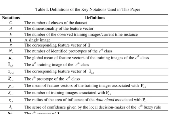
Table I. Definitions of the Key Notations Used in This Paper
Notations Definitions
C The number of classes of the dataset d The dimensionality of the feature vector
k The number of the observed training images/current time instance
I A single image
x The corresponding feature vector of I
c
N The number of identified prototypes of the cth class c
The global mean of feature vectors of the training images of the cth class ,
c k
I The kth training image of the cth class ,
c k
x The corresponding feature vector of Ic k,
, c i
P The ith prototype of the cth class ,
c i
p The mean of feature vectors of the training images associated with Pc i,
, c i
S The number of training images associated withPc i,
, c i
r The radius of the area of influence of the data cloud associated withPc i,
c
The score of confidence given by the local decision-maker of the cth fuzzy rule i
Sg The ith segment of I
3. Feature Extraction
In this section, we will briefly describe the feature descriptors that are employed in the DRB classifier to make it self-contained. Feature extraction can be viewed as a projection from the original images to a feature space that makes the images from different classes separable, namely, Ix. Current feature descriptors can be divided into three categories based on their descriptive abilities [44], namely: “low-level”, “medium-level” and “high-level”. Different feature descriptors have different advantages. In general, low-level feature descriptors work very well on problems where low-level visual features, e.g., spectral, texture, and structure, play the dominant role. In contrast, level feature descriptors work better on classifying images with high-diversity and nonhomogeneous spatial distributions because they can learn more abstract and discriminative semantic features.
In this paper, two low-level feature descriptors (GIST and HOG) are employed, and we further create a combination of both to improve their descriptive ability. However, as the low-level feature descriptors are not enough to handle efficiently complex, large-scale problems, we also use one of the most widely used high-level feature descriptors (a pre-trained VGG-VD-16 [42]). It has to be stressed that the high-level feature descriptor is directly used without further tuning and is a part of the pre-processing layer.
As there is no interdependence of different images within the feature extraction stage, it can be parallelized massively to further reduce the processing time. Once the global features (either low- or high-level) of the image are extracted and stored, there is no need to repeat the same process again.
We also have to stress that this paper describes a general DRB approach and the feature descriptors are not necessarily limited to GIST or HOG or the pre-trained VGG-VD-16 only. Alterative feature descriptors can be used, i.e. CaffeNet [22], SIFT [34], etc., and further combinations of different visual features can also be considered as well. One may further consider to refine the commonly used visual features into more informative representations by uncovering an appropriate latent subspace [30]. However, selecting the most suitable feature descriptor(s) for a particular problem requires prior knowledge about the problem, and this is out of the scope of this paper.
3.1. Employed Low-Level Feature Descriptors
A. GIST DescriptorGIST feature descriptor gives an impoverished and coarse version of the principal contours and textures of an image [38]. In the proposed DRB classifier, we use the same GIST descriptor as described in [38] without any modification, which extracts a 1 512 dimensional feature vector denoted byg
I g1
I ,g2 I ,...,
512 g I .B. HOG Descriptor
HOG descriptor [14] has been proven to be very successful in various computer vision tasks, such as object detection, texture analysis and image classification. In the DRB classifier, although the size of the images varies for different problems, we used the default block size of 2 2 and changed the cell size to fix the dimensionality of the HOG features to be 1 576 , denoted by h
I =h1
I ,h2
I ,...,h576
I .To improve the distinctiveness of the HOG feature vectors of images between different classes, we expand the value range of the HOG vectors by the following nonlinear nonparametric function [4],[5]:
2
sgn(1 ) exp 1 sgn(1 ) 1 exp 1 x x x x (1) where 1, 0 sgn( ) 0, 0 1, 0 x x x x , and the nonlinearly mapped HOG feature vector of I is denoted by
h
I
.C. Combined GIST-HOG Features
To further improve the descriptive ability of the GIST and HOG feature descriptors, in this paper, we further combine the GIST and HOG feature vectors to create a new, more descriptive integrated vector as follows:
, I I I I I h g f g h (2)where denotes the norm.
3.2. Employed High-Level Feature Descriptor
The VGG-VD-16 [42] is currently one of the best performing pre-trained DCNN feature descriptors widely used in different works. It has a simpler structure, but is able to provide better performance on various problems. We use the pre-trained VGG-VD-16 model as the high-level feature descriptor without any tuning to enhance the ability of the proposed DRB classifier in handling complex, large-scale, high-density image classification problems. Following the common practice, the 1×4096 dimensional activations from the first fully connected layer are extracted as the feature vector of the image I, denoted by v
I v1
I ,v2 I ,...,v4096
I .However, as the pre-trained model requires the input image to be the size of 227×227 pixels, it is, in fact, not good in handling problems with small-size images with simple semantic contents.
4. Massively Parallel Fuzzy Rule Base
In the DRB classifier, we employ a non-parametric rule-base formed of 0-order AnYa type fuzzy rules [3],[7], which makes the proposed classifier interpretable and transparent for human understanding (even to a non-expert) unlike the mainstream deep learning [10],[12],[13],[18],[20],[21],[26],[42]. Because of the prototype-based nature, the DRB classifier is free from prior assumptions about the type of distribution as well as the random or deterministic nature of data [6], the requirements of setting ad hoc model structure, handcrafting membership functions, etc. Meanwhile, the prototype-based nature further allows the DRB classifier a non-parametric, non-iterative, self-organising, self-evolving and highly parallel underlying structure
[2],[7], [8]. Thus, the training of the proposed DRB classifiers is fully autonomous, significantly faster and can start “from scratch” [2].
As described in more detail later in this section as well as in [3] and [6], the system automatically identifies prototypes from the empirically observed data (images) and forms data clouds (cluster-like groups of points with no predetermined shape) resembling Voronoi tessellation [37] per class. Thus, for a training dataset, which consists of C classes, C independent 0-order IF…THEN… FRB subsystems are generated (one per class) in parallel. Once the training process is finished, each subsystem generalizes/learns one 0-order AnYa type fuzzy rule corresponding to its own class based on the identified prototypes:
c,1
~ c N, c
IF I~P OR OR I P THEN class c (3) where “~” denotes similarity, which can also be seen as a fuzzy degree of satisfaction/membership [7] or typicality [6]; I is a particular image and x is its corresponding feature vector; x can be g
I ,
h
I
,
If or v
I ; Pc j, is the jth visual prototype of the cth class; pc j, is the corresponding feature vector of Pc j,and has the same dimensionality as x; j1, 2,...,Nc; Nc is the number of prototypes of the cth class. 1, 2,...,
c C.
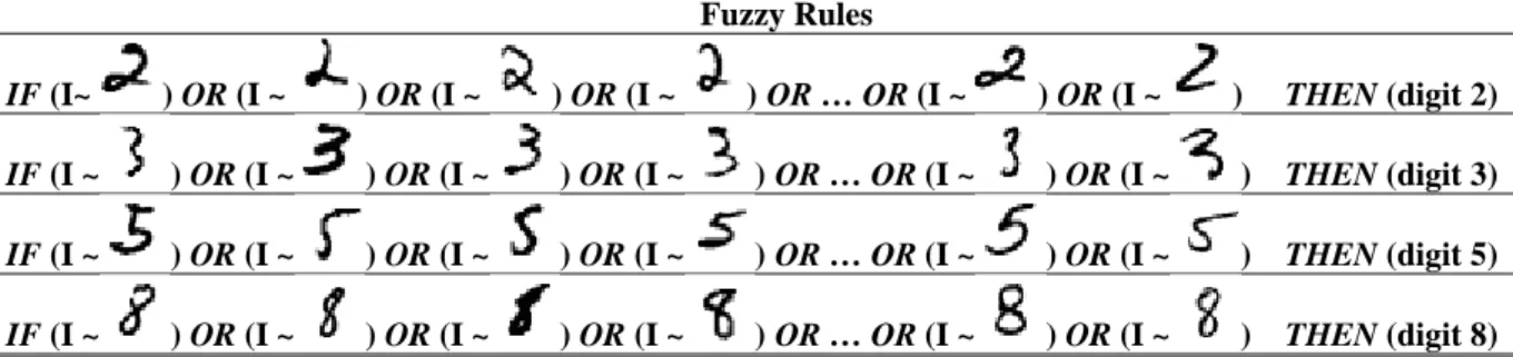
Examples of AnYa type fuzzy rules generalized from the popular handwritten digits recognition problem, MNIST dataset [27] for digits “2”, “3”, “5” and “8” are visualized in Table II. As we can see, AnYa type fuzzy rules in the table provide a very intuitive representation of the mechanism. Moreover, each of the AnYa type fuzzy rules can be interpreted as a number of simpler fuzzy rules with single prototype connected by “OR” operator. As a result, a massive parallelization is possible.
Table II. Illustrative Example of AnYa Fuzzy Rules with MNIST Dataset
Fuzzy Rules
IF (I~ ) OR (I ~ ) OR (I ~ ) OR (I~ ) OR … OR (I~ ) OR (I~ ) THEN (digit 2)
IF (I~ ) OR (I~ ) OR (I~ ) OR (I~ ) OR … OR (I~ ) OR (I~ ) THEN (digit 3)
IF (I~ ) OR (I~ ) OR (I~ ) OR (I~ ) OR … OR (I~ ) OR (I~ ) THEN (digit 5)
IF (I~ ) OR (I~ ) OR (I~ ) OR (I~ ) OR … OR (I~ ) OR (I~ ) THEN (digit 8)
In the remainder of this section, we will describe the training and validation processes as well as the decision-making mechanism of the proposed DRB classifier.
4.1. Training of the DRB System
Due to the highly parallel structure of the proposed system, in this subsection, we summarize the main procedure of the training process of a single FRB subsystem, namely the cthone.
Stage 0: System Initialization
The cth FRB subsystem is initialized by the first image of the cth class, Ic,1. We firstly apply the vector normalization to the global feature vector of Ic,1, denoted by xc,1(xc,1 xc,1,1,xc,1,2,...,xc,1,d, d is the dimensionality):
,1 ,1 ,1
c c c
x x x (4) With the vector normalization, the Euclidean distance between two normalized data samples z z and y y can be converted to cosine dissimilarity as follows: z z y y 2 1 cos
z y,
, where z y, is the angle between z and y. The vector normalization operation helps to overcome the so-called “curse of dimensionality” [1].Then, the meta-parameters of the system are initialized as follows: ,1 , ,1 , ,1 , , 1; ; 1; ; ; 1; ; c c c c c c c c N c c N c c N c N o k x N P I p x S r r (5) where k is the current time instance; c is the global mean of all the observed data samples of the cthclass;
, c
c N
p is the mean of feature vectors of the images associated with the first data cloud with the visual prototype , c
c N
P ; ,
c
c N
S is the number of images associated with the data cloud; ,
c
c N
r is the radius of the area of the data cloud; ro is a small value to stabilize the initial status of the newly formed data clouds. Data clouds are very much like clusters, but are nonparametric and do not have a specific pre-determined, regular shape. They directly represent the local ensemble properties of the observed data samples [7].
In this paper, we use 2 1 cos(30 )
o
or to define the degree of similarity on the edge of the data cloud. We need to stress that, ro is not a problem-specific parameter and requires no prior knowledge to be determined
Stage 1: Preparation
For the newly arrived kth (k k 1) training image that belongs to the cth class, denoted by Ic k, we firstly apply the vector normalization (expression (4)) to its corresponding feature vector: , ,
, c k c k c k x x x . Then,
the global mean, c is updated as follows:
, 1 1 c c c k k k k x (6) And we calculate the data densities of all the existing prototypes Pc i, (i1, 2,...,Nc, whereNc is the number of identified prototypes) as detailed in [6]:
, 2 2 , 1 1 c i c i c c D P p (7a)as well as the data density of the new image Ic k, :
, 2 2 , 1 1 c k c k c c D I x (7b)where c2 Xc c 2 1 c 2; Xc is the average norm of the observed normalized data samples, which is always equal to 1 due to the vector normalization operation.
Stage 2: System Update
In this stage, we update the system structure and meta-parameters to accommodate the newly arrived image. Firstly, Condition 1 is checked to see whether Ic k, becomes a new prototype:
Condition 1:
, , , 1,2,..., , 1,2,..., , max min c c c k c i c k j N c i j N c k IF D D OR D DTHEN is a new prototype
I P I P I (8)
Once Condition 1 is satisfied, Ic k, is set to be a new prototype and it initializes a new data cloud:
, , , , , ,
1; ; ; 1; ;
c c c c
c c c N c k c N c k c N c N o
N N P I p x S r r (9)
If Condition 1 is not met, we find the nearest prototype to Ic k, , denoted byPc n, , using equation (10):
, , , 1,2,..., arg min c c n c k c j j N P x p (10)Before we associate Ic k, with the data cloud of Pc n, , Condition 2 is checked to see whether Ic k, locates in the area of influence of Pc n, :
Condition 2:
, , ,
, ,
c
c k c n c N c k c n
IF x p r THEN I is assigned toP (11)
If Condition 2 is met, Ic k, is assigned to the data cloud formed around the prototype Pc n, and the
meta-parameters of this data cloud are updated as follows:
, 2 2 2 , , , , , , , , , , 1 1 1 1 1; ; ; 2 2 c n c n c n c n c n c k c n c n c n c n c n S S S r r S S p p x (12) where 2 2 , 1 , c n c n
p .Otherwise, it means that Ic k, is out of the influence area of the nearest data cloud, and, therefore, a new data cloud is initialized by Ic k, with Ic k, as its prototype (Nc Nc1). The meta-parameters of the new data cloud
are, then, added using expression (9).
Then, the next image is grabbed at Stage 1. After all the training samples have been processed, the system goes to the final stage and generates the AnYa type fuzzy rule.
Stage 3: Fuzzy Rules Generation
Once the training process has been finished, the system will generate one AnYa fuzzy rule based on the identified prototypes: c Rule :
,1
,
c c c N IF I~P OR OR I~P THEN class c (13) If more training samples are available later, the FRB subsystem can continue the processing cycle from Stage 1 and update the fuzzy rules accordingly.Fig. 2. Flowchart of the training process of the FRB subsystem
4.2. Classifying with the Identified FRB System
After the identification procedure, the FRB system generates C fuzzy rules in regards to the C classes. For each testing image I, each one of the C fuzzy rules will generate a score of confidence c
I by its local (per rule) decision-maker based on the feature vector of I, denoted by x:
2
, 1,2,...,
arg max exp
c c c j j N I x p (14)
As a result, one can get C scores of confidence
I 1
I ,2 I ,...,C
I per image, which are the inputs of the overall decision-maker of the DRB classifier.4.3. Decision-Making Mechanism
For a single FRB system, the overall decision-maker (the last layer in Fig. 1) decides the label of the validation image using the “winner-takes-all” principle as follows:
1,2,..., arg max c c C label I I (15) In some applications, i.e. face recognition, remote sensing, object recognitions, etc., where local information may play a more important role than the global information, one can consider segmenting (both the training and validation) images to capture local information. In such cases, the 0-order FRB subsystems are trained with segments of training images instead of the full images. The overall label of a validation image is given as an integration of all the scores of confidence that the FRB subsystems associated with its segments, denoted by Sg1,Sg2,…,SgT :
1,2,..., 1 1 arg max T c i c C i label T
I Sg (16) If an FRB ensemble [23] is used, the label of the validation image is considered as the integration of all the scores of confidence that the FRB systems given to the image [4]:
,
,
1,2,..., 1,2,..., 1
1
arg max max
K c i c i i K c C i label K
I I I (17) where K is the number of FRB systems in the ensemble.5. Numerical Examples and Discussions
In this section, we study the performance of the proposed DRB classifier. All the numerical examples are conducted using Matlab2017a on a PC with dual core i7 processor with clock frequency 3.4GHz each and 16GB RAM.
To illustrate the proposed DRB classifier, we consider the following four well-known benchmark datasets covering three different challenging problems:
1) MNIST dataset for handwritten digits recognition [27]; 2) Singapore dataset for remote sensing [17];
3) UCMerced dataset for remote sensing [47]; 4) Caltech101 dataset for object recognition [16].
We then compare the results with the state-of-the-art approaches. As the four benchmark datasets are very different from each other, we will use four different, but same as in the publications [17], [18], [27] experimental protocols for each dataset, respectively.
5.1. MNIST Dataset
The MNIST dataset [27] is a famous benchmark database for handwritten digits recognitions that contains 70000 grey images (60000 of them form the training set and 10000 are used for validation) of handwritten digits (“0” to “9”). The image size is 28 28 for both the training and validation images.
There is a large number of publications reporting highly accurate results. However, due to the fact that the dataset itself has flaws, there are a number of validation images with unrecognizable digits even for humans (see Fig. 3), the testing accuracy is below 100%, although closely approaching it, see table III.
Fig.3. The only 56 mistakes made by the DRB Ensemble out of 10000 validation images
The detailed architecture of the proposed DRB for handwritten digits recognition for the training process is shown in Fig.4. The architecture for the validation process is given in Fig.5.
Fig.4. Architecture for training (handwritten digits recognition)
Fig.5. Architecture for validation (handwritten digits recognition)
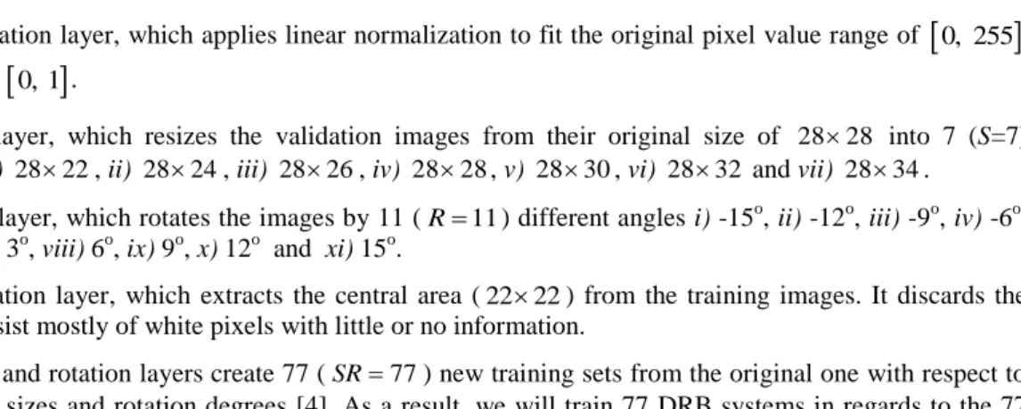
The pre-processing block of the proposed DRB classifier for handwritten digits recognition consists of the following layers, where we adopt the same rotation and scaling operation as used in references [12], [13] but without using elastic distortion:
1. Normalization layer, which applies linear normalization to fit the original pixel value range of
0, 255
into the range of
0, 1 .2. Scaling layer, which resizes the validation images from their original size of 28 28 into 7 (S=7) different sizes: i) 28 22 , ii) 28 24 , iii) 28 26 , iv) 28 28 , v) 28 30 , vi) 28 32 and vii) 28 34 .
3. Rotation layer, which rotates the images by 11 (R11) different angles i) -15o, ii) -12o, iii) -9o, iv) -6o,
v) -3o, vi) 0o, vii) 3o, viii) 6o, ix) 9o, x) 12o and xi) 15o.
4. Segmentation layer, which extracts the central area ( 22 22 ) from the training images. It discards the borders that consist mostly of white pixels with little or no information.
The scaling and rotation layers create 77 (SR77) new training sets from the original one with respect to different scaling sizes and rotation degrees [4]. As a result, we will train 77 DRB systems in regards to the 77 new training sets and later form an ensemble. Each DRB system consists of 10 AnYa type 0-order fuzzy rules with a large number of prototypes connected with a disjunction (Logical “OR”) as shown in Table II, corresponding to digits “0” to “9”. For each validation image, we just apply the normalization and segmentation operations.
Since the images within the MNIST dataset are quite small and simple, high-level feature descriptors are not suitable for this problem. Therefore, the feature descriptor used by the DRB classifier in this experiment is GIST, HOG or the combined GIST and HOG (CGH) features. However, due to the different descriptive abilities of these features, the performance of the DRB classifier is somewhat different. The recognition accuracy of the proposed DRB classifier using different feature descriptors is tabulated in Table III. The corresponding average training times for the 10 fuzzy rules are tabulated in Table IV.
Table III. Comparison between the Proposed Approach and the State-of-the-Art Approaches
Approaches DRB-GIST DRB-HOG DRB- CGH DRB Ensem ble DRB Cascade [5] Large Convolution al Networks [40] Large Convolution al Networks [21] Committee of 7 Convolution al Neural Networks [12] Committee of 35 Convolution al Neural Networks [13] Accuracy 99.30% 98.86% 99.32% 99.44 % 99.55% 99.40% 99.47% 99.73% 2% 99.77%
Training Time Less than 2 minute for each part
No Information
No Information
Almost 14 hours for each one of the DNNs.
PC-Parameters Core i7-4790 (3.60GHz), 16 GB DDR3 Core i7-920 (2.66GHz), 12
GB DDR3
GPU Used None 2 2 GTX 480 & GTX 580 Elastic
Distortion No No No Yes
Tuned
Parameters No Yes Yes Yes
Iteration No Yes Yes Yes
Randomness No Yes Yes Yes
Parallelization Yes No No No
Evolving
Ability Yes No No No
By further creating a DRB ensemble consisting of a DRB classifier trained with GIST features and a DRB classifier trained with HOG features, we achieve a better recognition performance, which is tabulated in Table III as well. In our previous work, we also proposed a DRB cascade [5] that further improves the recognition accuracy by using a SVM for conflict resolution, which is also presented in Table III. The conflict resolution only applies to a small number (about 5%) of the validation data for which the two highest confidence values are close to each other and thus there may be two possible winners with similar overall scores [5]. One of the
important advantages of the proposed DRB classifier is that it provides in a clear and explicit form per rule/class confidence level.
The only 56 images that are incorrectly recognized by the proposed DRB ensemble are depicted in Fig. 3 and the corresponding labels are given on top of these images. As we can see, none of these digits is written clearly and the majority of them are far different from the normal handwriting styles.
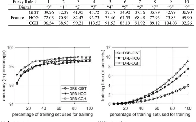
One of the most distinctive advantages of the proposed DRB classifier is its evolving ability, which means that there is no need for complete re-training of the classifier when new data samples are available. To illustrate this advantage, we train the DRB classifier with images in the form of an image stream (video). Meanwhile, the execution time and the recognition accuracy are recorded during the process. In this example, we use the original training set without rescaling or rotation, which speeds up the process significantly. The relationship curves of the training time (the average for each of the 10 fuzzy rules) and recognition accuracy with the growing amount of the training samples are depicted in Fig. 6.
Table IV. Computation Time for the Learning Process per Sub-system (in seconds)
Fuzzy Rule # 1 2 3 4 5 6 7 8 9 10 Digital “0” “1” “2” “3” “4” “5” “6” “7” “8” “9” Feature GIST 39.26 32.39 41.95 45.72 37.17 34.90 37.36 35.89 42.99 36.90 HOG 72.03 70.99 82.47 92.73 73.46 67.53 68.48 77.93 75.83 69.90 CGH 96.54 88.93 99.21 113.52 91.53 85.19 91.92 89.12 104.08 92.26 (a) Accuracy (b) Training time
Fig.6.The relationship curve of training time and recognition accuracy with different amount of training samples In order to evaluate the performance of the proposed DRB classifier, we also present the state-of-the-art approaches reporting the current best and the second best published results (with and without elastic distortion) worldwide in Table III.
As we can see, the approaches reported in [12], [13] using elastic distortion can achieve slightly better results than the approaches [21], [40] as well as the proposed DRB classifier. However, this comes at a price of using elastic distortion. This kind of distortion exhibits a significant randomness that may turn an unrecognizable digit into a recognizable one and vice versa, which also casts doubt on the effectiveness of the approaches in real-world applications. In addition, elastic distortion puts in question the achieved results’ repeatability and requires a cross-validation that further obstructs online applications and the reliability of the results [4].
Without using elastic distortion, the current published best result is 99.47% [21], which is comparable with the proposed DRB ensemble, but worse than the DRB cascade [5]. However, one needs to notice that the DCNNs require a large number of parameters (tens or hundreds of millions) to be optimized, hugely longer time and more complex accelerated hardware, cannot start “from scratch”, cannot evolve with the data stream and are not human-interpretable.
5.2. Singapore Dataset
Singapore dataset was constructed from a large satellite image of Singapore [17]. This dataset consists of 1086 images with 256 × 256 pixels size with 9 scene categories: i) airplane, ii) forest, ii) harbor, iv) industry, v)
meadow, vi) overpass, vii) residential, viii) river, and ix) runway. Examples of images of the 9 classes are given in Fig.7.
Fig.7. Examples of images from the Singapore dataset
The architecture of the proposed DRB classifier, as shown in Fig.8, consists of the following layers: 1. Normalization layer;
2. Rotation layer, which rotates the images by i) 0o, ii) 90 o, iii) 180 o and iv) 270o to improve the generalization ability of the classifier.
3. Segmentation layer, which splits each image into smaller pieces by a 64 64 size sliding window with the step size of 32 pixels in both horizontal and vertical directions. The segmentation layer cuts one image into
49 pieces.
4. Feature descriptor, which extracts the combined GIST and HOG features from each segment.
5. FRB system, which consists of 9 fuzzy rules, each of them is trained based on the segments of images of a particular class within the dataset.
6. Decision-maker, which generates the labels using equation (16).
Fig.8. Architecture for remote sensing (with low-level feature descriptors)
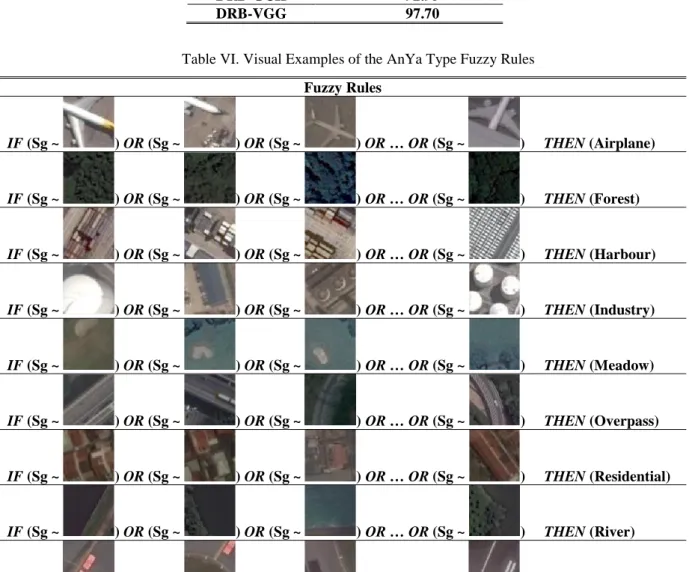
Following the commonly used experimental protocol [17], we firstly transform the images into grey-level ones and train the proposed DRB classifier with randomly selected 20% of images of each class and use the remainder as a validation data set. The experiment is repeated 5 times and the average accuracy is reported in Table V. Visual examples of the extracted IF…THEN… rules per class during experiments are given in Table VI.
The performance of the proposed DRB is also compared with the state-of-the-art approaches as follows: 1. Transfer Learning with Deep Representations (TLDP) [41];
3. Bag of Visual Words (BoVW) [47];
4. Scale-Invariant Feature Transform with Sparse Coding (SIFTSC) [11]; 5. Spatial Pyramid Matching Kernel (SPMK) [25].
and the recognition accuracies of the comparative approaches are reported in Table V as well. One can see that, the proposed approach is able to produce a significantly better recognition result than the best current methods. Furthermore, by using a smaller step size, the DRB classifier can grasp more details, and this leads to a better recognition performance.
Table V. Comparison between the Proposed Approach and the State-of-the-Art Approaches
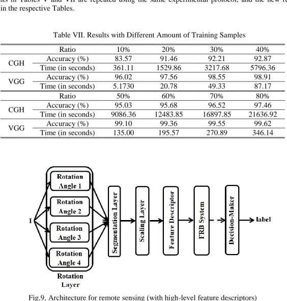
Method Accuracy (%) TLDP [41] 82.13 TLFP [17] 90.94 BoVW [47] 87.41 SIFTSC [11] 87.58 SPMK [25] 82.85 DRB-GCH 92.95 DRB-VGG 97.70
Table VI. Visual Examples of the AnYa Type Fuzzy Rules
Fuzzy Rules IF (Sg ~ ) OR (Sg ~ ) OR (Sg ~ ) OR… OR (Sg~ ) THEN (Airplane) IF (Sg ~ ) OR (Sg~ ) OR (Sg~ ) OR … OR (Sg~ ) THEN (Forest) IF (Sg~ ) OR (Sg~ ) OR (Sg~ ) OR … OR (Sg~ ) THEN (Harbour) IF (Sg~ ) OR (Sg~ ) OR (Sg~ ) OR … OR (Sg~ ) THEN (Industry) IF (Sg~ ) OR (Sg~ ) OR (Sg~ ) OR … OR (Sg~ ) THEN (Meadow) IF (Sg~ ) OR (Sg~ ) OR (Sg~ ) OR … OR (Sg~ ) THEN (Overpass) IF (Sg~ ) OR (Sg~ ) OR (Sg~ ) OR … OR (Sg~ ) THEN (Residential) IF (Sg~ ) OR (Sg~ ) OR (Sg~ ) OR … OR (Sg~ ) THEN (River) IF (Sg~ ) OR (Sg ~ ) OR (Sg~ ) OR … OR (Sg ~ ) THEN (Runway)
To show the evolving ability of the proposed DRB classifier, we randomly select out 20% of the images of each class for validation and train the DRB classifier with 10%, 20%, 30%, 40%, 50%, 60%, 70% and 80% of the dataset. The experiment is repeated five times and the average accuracy is tabulated in Table VII. The
average time for training is also reported, however, due to the unbalanced classes, the training time as tabulated in Table VII is the overall training time of the nine fuzzy rules.
As handwritten digits images in the MNIST dataset are much simpler, the low-level feature descriptors are sufficient for problems of this type. In contrast, remote sensing images have more fine details and a variety of semantic contents. Therefore, we further introduce the high-level feature descriptor, namely, the pre-trained VGG-VD-16 model, into the DRB classifier and use the original RGB remote sensing images for training. The architecture of the DRB classifier is adjusted as depicted in Fig. 9 to accommodate the high-level feature descriptor. As one can see, the adjusted DRB classifier is different from the one using low-level feature descriptors in terms of the following layers:
1. Segmentation layer, which splits each image into smaller pieces by a 192 192 pixels size sliding window with the step size of 64 pixels in both horizontal and vertical directions. The segmentation layer cuts one image into 4 pieces.
2. Scaling layer, which resizes the image segments into the size of 227 227 pixels;
3. Feature descriptor, which extracts a 1 4096 dimensional feature vector from each segment;
And the rotation layer, FRB layer and decision makers are the same as shown in Fig. 8. Then, the experiments in Tables V and VII are repeated using the same experimental protocol, and the new results are tabulated in the respective Tables.
Table VII. Results with Different Amount of Training Samples
Ratio 10% 20% 30% 40%
CGH Accuracy (%) 83.57 91.46 92.21 92.87
Time (in seconds) 361.11 1529.86 3217.68 5796.36
VGG Accuracy (%) 96.02 97.56 98.55 98.91
Time (in seconds) 5.1730 20.78 49.33 87.17
Ratio 50% 60% 70% 80%
CGH Accuracy (%) 95.03 95.68 96.52 97.46
Time (in seconds) 9086.36 12483.85 16897.85 21636.92
VGG Accuracy (%) 99.10 99.36 99.55 99.62
Time (in seconds) 135.00 195.57 270.89 346.14
Fig.9. Architecture for remote sensing (with high-level feature descriptors)
From the above experiments one can see that by using the high-level feature descriptor, both the recognition accuracy and the computational efficiency of the DRB classifier on the remote sensing problem are significantly boosted.
5.3. UCMerced Dataset
UCMerced dataset [47] consists of fine spatial resolution remote sensing images of 21 challenging scene categories (including airplane, beach, building, etc.). Each category contains 100 images of the same image size (256×256 pixels). The example images of the 21 classes are shown in Fig.10.
Following the commonly used experimental protocol [17], we randomly select 80% of images of each class for training and use the remainder as a validation set. The experiment is repeated 5 times and the average accuracy is reported in Table VIII. In this experiment, we use the same architecture as depicted in Fig. 9.
The performance of the proposed DRB is also compared with the state-of-the-art approaches as follows: 1. Two-Level Feature Representation (TLFP) [17];
2. Bag of Visual Words (BoVW) [47];
3. Scale-Invariant Feature Transform with Sparse Coding (SIFTSC) [11]; 4. Spatial Pyramid Matching Kernel (SPMK) [25],[48];
5. Multipath Unsupervised Feature Learning (MUFL) [15]; 6. Random Convolutional Network (RCNet) [50];
7. Linear SVM with Pre-Trained CaffeNet (SVM+Caffe) [39];
8. LIBLINEAR Classifier with the VGG-VD-16 Features (LIBL+VGG) [44]; 9. Linear SVM with the VGG-VD-16 Features (SVM+VGG).
Fig.10. Example Images from the UCMerced dataset
Table VIII. Comparison between the Proposed Approach and the-State-of-the-Art Approaches
Approach Accuracy Approach Accuracy
TLFR [17] 91.12% RCNet [50] 94.53%
BoVW [47] 76.80% SVM+ Caffe [39] 93.42%
SIFTSC [11] 81.67% LIBL+VGG [44] 95.21%
SPMK [48] 74.00% SVM+VGG 94.48%
MUFL [15] 88.08% DRB 96.14%
From the comparison given in Table VIII one can see that, the proposed DRB classifier, again, produced the best classification performance. Similarly, we randomly select out 20% of the images of each class for validation and train the DRB classifier with 10%, 20%, 30%, 40%, 50%, 60% and 70% of the dataset. The experiment is repeated 5 times, and the average accuracy and time required for training (per rule) are tabulated in Table IX. One can see from Table X that the DRB classifier can achieve 95%+ classification accuracy with less than 20 seconds for training each fuzzy rule in addition to the highly interpretable structure and
Table IX. Results with Different Amount of Training Samples
Ratio 10% 20% 30% 40%
Accuracy (%) 83.48 88.57 90.80 92.19
Time (in seconds) 0.27 1.36 3.96 5.83
Ratio 50% 60% 70% 80%
Accuracy (%) 93.48 94.19 95.14 96.10
Time (in seconds) 10.29 11.52 15.49 18.15
5.4. Caltech101 Dataset
Caltech 101 dataset [16] contains 9144 pictures of objects belonging to 101 categories plus one background category. The number of images in each class varies from 33 to 800. The size of each image is roughly 300 200 pixels. This data set contains both classes corresponding to rigid object (like bikes and cars) and classes corresponding to non-rigid object (like animals and flowers). Therefore, the shape variance is significant. The examples of this dataset are presented in Fig. 11.
The architecture of the DRB classifier for object recognition is depicted in Fig. 12, which is the same as the latter part of the DRB classifier for remote sensing problems as presented in Fig. 9. The images of the Caltech 101 dataset [16] are very uniform in presentation, aligned from left to right, and usually not occluded, therefore, the rotation and segmentation are not necessary.
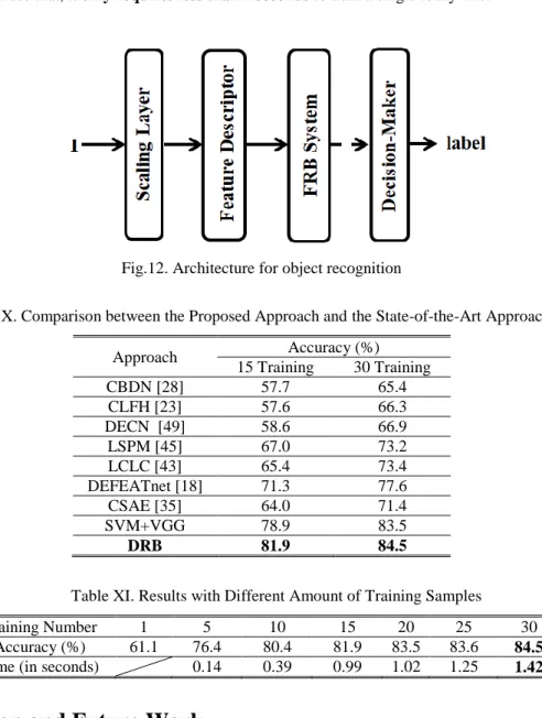
Following the commonly used protocol [18], we conduct the experiments by selecting 15 and 30 training images from each class and using the rest for validation. The experiment is repeated 5 times and the average accuracy is reported in Table X. We also compare the DRB classifier with the state-of-the-art approaches as follows:
1. Convolutional Deep Belief Network (CBDN) [28]; 2. Learning Convolutional Feature Hierarchies (CLFH) [23]; 3. Deconvolutional Networks (DECN) [49];
4. Linear Spatial Pyramid Matching (LSPM) [45]; 5. Local-Constraint Linear Coding (LCLC) [43]; 6. DEFEATnet [18];
7. Convolutional Sparse Autoencoders (CSAE) [35];
8. Linear SVM with the VGG-VD-16 Features (SVM+VGG).
Fig.11. Example images of the Caltech 101 dataset
As one can see from Table X that the DRB classifier easily outperforms all the comparative approaches in the object recognition problem. Same as the previous example, we randomly select out 1, 5, 10, 15, 20, 25, and 30 images of each class for training the DRB classifier and use the rest for validation. The experiment is
repeated 5 times, and the average accuracy and time consumption for training (per rule) are tabulated in Table XI, where we can see that, it only requires less than 2 seconds to train a single fuzzy rule.
Fig.12. Architecture for object recognition
Table X. Comparison between the Proposed Approach and the State-of-the-Art Approaches
Approach Accuracy (%) 15 Training 30 Training CBDN [28] 57.7 65.4 CLFH [23] 57.6 66.3 DECN [49] 58.6 66.9 LSPM [45] 67.0 73.2 LCLC [43] 65.4 73.4 DEFEATnet [18] 71.3 77.6 CSAE [35] 64.0 71.4 SVM+VGG 78.9 83.5 DRB 81.9 84.5
Table XI. Results with Different Amount of Training Samples
Training Number 1 5 10 15 20 25 30
Accuracy (%) 61.1 76.4 80.4 81.9 83.5 83.6 84.5
Time (in seconds) 0.14 0.39 0.99 1.02 1.25 1.42
6. Conclusion and Future Work
In this paper, a new powerful multilayer fuzzy rule-based (DRB) classifier for image recognition problems is proposed. It is a neuro-fuzzy architecture, but we stress its IF…THEN… highly interpretable rule-base aspect. Thanks to its prototype-based nature, the proposed approach can self-organize a transparent and human understandable fuzzy rule-based (FRB) system structure in a highly efficient way starting “from scratch”. Its one-pass type training process is non-parametric, entirely data-driven and fully automatic. Without any iteration, the DRB classifier is able to offer extremely high classification, comparable with human abilities and on par or surpassing best published mainstream deep learning alternatives. The proposed DRB classifier is a general approach for various problems and serves as a strong alternative to the state-of-the-art approaches by providing a fully human-interpretable structure after a very fast (in orders of magnitude faster than the mainstream deep learning methods), transparent, nonparametric training process. Numerical examples on four well-known benchmark datasets demonstrate the excellent performance and strong advantages of the proposed approach.
As future work, we are particularly interested in applying the DRB system on human face recognition problems. We will also apply the DRB system to other image processing problems and heterogeneous classification problems where the data are coming in different form (images/video, text/natural language as well as signals/physical variables). The convergence of the DRB systems will be studied as well. We are further interested to study collaborative scenarios whereby a set of distributed DRB classifiers exchange prototypes. Finally, we will also study the local optimality of the classifier structure.
Reference
[1] C. C. Aggarwal, A. Hinneburg, and D. A. Keim, “On the surprising behavior of distance metrics in high dimensional space,” in International Conference on Database Theory, 2001, pp. 420–434.
[2] P. Angelov, Autonomous learning systems: from data streams to knowledge in real time. John Wiley & Sons, Ltd., 2012.
[3] P. P. Angelov and X. Gu, “Autonomous learning multi-model classifier of 0-order (ALMMo-0),” in IEEE International Conference on Evolving and Autonomous Intelligent Systems, 2017, pp. 1–7. [4] P. P. Angelov and X. Gu, “MICE: Multi-layer multi-model images classifier ensemble,” in IEEE
International Conference on Cybernetics, 2017, pp. 436–443.
[5] P. Angelov and X. Gu, “A cascade of deep learning fuzzy rule-based image classifier and SVM,” in International Conference on Systems, Man and Cybernetics, 2017, pp. 1–8.
[6] P. P. Angelov, X. Gu, and J. Principe, “A generalized methodology for data analysis,” IEEE Trans. Cybern., DOI: 10.1109/TCYB.2017.2753880, 2017.
[7] P. Angelov and R. Yager, “A new type of simplified fuzzy rule-based system,” Int. J. Gen. Syst., vol. 41, no. 2, pp. 163–185, 2011.
[8] P. Angelov and X. Zhou, “Evolving fuzzy-rule based classifiers from data streams,” IEEE Trans. Fuzzy Syst., vol. 16, no. 6, pp. 1462–1474, 2008.
[9] R. G. Casey, “Moment Normalization of Handprinted Characters,” IBM J. Res. Dev., vol. 14, no. 5, pp. 548–557, 1970.
[10] K. Charalampous and A. Gasteratos, “On-line deep learning method for action recognition,” Pattern Anal. Appl., vol. 19, no. 2, pp. 337–354, 2016.
[11] A. M. Cheriyadat, “Unsupervised feature learning for aerial scene classification,” IEEE Trans. Geosci. Remote Sens., vol. 52, no. 1, pp. 439–451, 2014.
[12] D. Cireşan, U. Meier, L. M. Gambardella, and J. Schmidhuber, “Convolutional neural network committees for handwritten character classification,” in International Conference on Document Analysis and Recognition, 2011, vol. 10, pp. 1135–1139.
[13] D. Ciresan, U. Meier, and J. Schmidhuber, “Multi-column deep neural networks for image classification,” in Conference on Computer Vision and Pattern Recognition, 2012, pp. 3642–3649. [14] N. Dalal and B. Triggs, “Histograms of oriented gradients for human detection,” in IEEE Computer
Society Conference on Computer Vision and Pattern Recognition, 2005, pp. 886–893.
[15] J. Fan, T. Chen, and S. Lu, “Unsupervised feature learning for land-use scene recognition,” IEEE Trans. Geosci. Remote Sens., vol. 55, no. 4, pp. 2250–2261, 2017.
[16] L. Fei-Fei, R. Fergus, and P. Perona, “Learning generative visual models from few training examples: an incremental Bayesian approach tested on 101 object categories,” Comput. Vis. Image Underst., vol. 106, no. 1, pp. 59–70, 2007.
[17] J. Gan, Q. Li, Z. Zhang, and J. Wang, “Two-level feature representation for aerial scene classification,” IEEE Geosci. Remote Sens. Lett., vol. 13, no. 11, pp. 1626–1630, 2016.
[18] S. Gao, L. Duan, and I. W. Tsang, “DEFEATnet—A deep conventional image representation for image classification,” IEEE Trans. Circuits Syst. Video Technol., vol. 26, no. 3, pp. 494–505, 2016.
[19] S. Gao, Y. Zhang, K. Jia, J. Lu, and Y. Zhang, “Single Sample Face Recognition via Learning Deep Supervised Auto-Encoders,” IEEE Trans. Inf. Forensics Secur., vol. 6013, no. c, pp. 1–1, 2015. [20] I. Goodfellow, Y. Bengio, and A. Courville, Deep learning. Crambridge, MA: MIT Press, 2016. [21] K. Jarrett, K. Kavukcuoglu, M. Ranzato, and Y. LeCun, “What is the best multi-stage architecture for
object recognition?,” in IEEE International Conference on Computer Vision, 2009, pp. 2146–2153. [22] Y. Jia, E. Shelhamer, J. Donahue, S. Karayev, J. Long, R. Girshick, S. Guadarrama, and T. Darrell,
“Caffe: convolutional architecture for fast feature embedding∗,” in ACM International Conference on Multimedia, 2014, pp. 675–678.
[23] K. Kavukcuoglu, P. Sermanet, Y.-L. Boureau, K. Gregor, M. Mathieu, and Y. LeCun, “Learning convolutional feature hierarchies for visual recognition,” in Advances in neural information processing systems, 2010, pp. 1090–1098.
[24] L. Kuncheva, Combining pattern classifiers: methods and algorithms. Hoboken, New Jersey: John Wiley & Sons, 2004.
[25] S. Lazebnik, C. Schmid, and J. Ponce, “Beyond bags of features : spatial pyramid matching for recognizing natural scene categories,” in IEEE Computer Society Conference on Computer Vision and Pattern Recognition, 2006, pp. 2169–2178.
[26] Y. LeCun, Y. Bengio, and G. Hinton, “Deep learning,” Nat. Methods, vol. 13, no. 1, pp. 35–35, 2015. [27] Y. LeCun, L. Bottou, Y. Bengio, and P. Haffner, “Gradient-based learning applied to document
recognition,” Proc. IEEE, vol. 86, no. 11, pp. 2278–2323, 1998.
[28] H. Lee, R. Grosse, R. Ranganath, and A. Y. Ng, “Convolutional deep belief networks for scalable unsupervised learning of hierarchical representations,” in Annual International Conference on Machine Learning, 2009, pp. 1–8.
[29] T. M. Lehmann, C. Gönner, and K. Spitzer, “Survey: interpolation methods in medical image processing,” IEEE Trans. Med. Imaging, vol. 18, no. 11, pp. 1049–1075, 1999.
[30] Z. Li, J. Liu, J. Tang, and H. Lu, “Robust structured subspace learning for data representation,” IEEE Trans. Pattern Anal. Mach. Intell., vol. 37, no. 10, pp. 2085–2098, 2015.
[31] Z. Li and J. Tang, “Weakly supervised deep metric learning for community-contributed image retrieval,” IEEE Trans. Multimed., vol. 17, no. 11, pp. 1989–1999, 2015.
[32] Z. Li and J. Tang, “Weakly supervised deep matrix factorization for social image understanding,” IEEE Trans. Image Process., vol. 26, no. 1, pp. 276–288, 2017.
[33] F. Liu, J. Tang, Y. Song, Y. Bi, and S. Yang, “Local structure based multi-phase collaborative representation for face recognition with single sample per person,” Inf. Sci. (Ny)., vol. 346–347, pp. 198–215, 2016.
[34] D. G. Lowe, “Distinctive image features from scale-invariant keypoints,” Int. J. Comput. Vis., vol. 60, no. 2, pp. 91–110, 2004.
[35] W. Luo, J. Li, J. Yang, W. Xu, and J. Zhang, “Convolutional sparse autoencoders for image classification,” IEEE Trans. Neural Networks Learn. Syst., pp. 1–6, 2017.
[36] V. Mnih, K. Kavukcuoglu, D. Silver, A. A. Rusu, J. Veness, M. G. Bellemare, A. Graves, M. Riedmiller, A. K. Fidjeland, G. Ostrovski, S. Petersen, C. Beattie, A. Sadik, I. Antonoglou, H. King, D. Kumaran, D. Wierstra, S. Legg, and D. Hassabis, “Human-level control through deep reinforcement learning,” Nature, vol. 518, no. 7540, pp. 529–533, 2015.
[37] A. Okabe, B. Boots, K. Sugihara, and S. N. Chiu, Spatial tessellations: concepts and applications of Voronoi diagrams, 2nd ed. Chichester, England: John Wiley & Sons., 1999.
[38] A. Oliva and A. Torralba, “Modeling the shape of the scene: A holistic representation of the spatial envelope,” Int. J. Comput. Vis., vol. 42, no. 3, pp. 145–175, 2001.
[39] A. B. Penatti, K. Nogueira, and J. A. Santos, “Do deep features generalize from everyday objects to remote sensing and aerial scenes domains ?,” in IEEE Conference on Computer Vision and Pattern Recognition, 2015, pp. 44–51.
[40] M. Ranzato, F. J. Huang, Y. L. Boureau, and Y. LeCun, “Unsupervised learning of invariant feature hierarchies with applications to object recognition,” in Proceedings of the IEEE Computer Society Conference on Computer Vision and Pattern Recognition, 2007, pp. 1–8.
[41] A. B. Sargano, X. Wang, P. Angelov, and Z. Habib, “Human Action Recognition using Transfer Learning with Deep Representations,” in IEEE International Joint Conference on Neural Networks (IJCNN), 2017, pp. 463–469.
[42] K. Simonyan and A. Zisserman, “Very deep convolutional networks for large-scale image recognition,” in International Conference on Learning Representations, 2015, pp. 1–14.
[43] J. Wang, J. Yang, K. Yu, F. Lv, T. Huang, and Y. Gong, “Locality-constrained linear coding for image classification,” in IEEE Conference on Computer Vision and Pattern Recognition, 2010, pp. 3360– 3367.
[44] G. S. Xia, J. Hu, F. Hu, B. Shi, X. Bai, Y. Zhong, and L. Zhang, “AID: A benchmark dataset for performance evaluation of aerial scene classification,” IEEE Trans. Geosci. Remote Sens., vol. 55, no. 7, pp. 3965–3981, 2017.
[45] J. Yang, K. Yu, Y. Gong, and T. Huang, “Linear spatial pyramid matching using sparse coding for image classification,” in IEEE Conference on Computer Vision and Pattern Recognition, 2009, pp. 1794–1801.
[46] M. Yang, X. Wang, G. Zeng, and L. Shen, “Joint and collaborative representation with local adaptive convolution feature for face recognition with single sample per person,” Pattern Recognit., vol. 66, no. July 2016, pp. 117–128, 2017.
[47] Y. Yang and S. Newsam, “Bag-of-visual-words and spatial extensions for land-use classification,” in International Conference on Advances in Geographic Information Systems, 2010, pp. 270–279. [48] Y. Yang and S. Newsam, “Spatial pyramid co-occurrence for image classification,” in Proceedings of
the IEEE International Conference on Computer Vision, 2011, pp. 1465–1472.
[49] M. Zeiler, D. Krishnan, G. Taylor, and R. Fergus, “Deconvolutional networks,” in IEEE Conference on Computer Vision and Pattern Recognition, 2010, pp. 2528–2535.
[50] L. Zhang, L. Zhang, and V. Kumar, “Deep learning for remote sensing data,” IEEE Geosci. Remote Sens. Mag., vol. 4, no. 2, pp. 22–40, 2016.