Real-time pre-processing technique for drift detection, feature tracking, and feature selection using adaptive micro-clusters for data stream classification

(1)

Detection, Feature Tracking, and Feature Selection

using Adaptive Micro-Clusters for Data Stream

Classification

Thesis Submitted for the Degree of Doctor of Philosophy,

School of Mathematical, Physical, and Computational Sciences

by

Mahmood Shakir Hammoodi

Supervisor: Dr. Frederic Stahl

(2)

Data streams are unbounded, sequential data instances that are generated with high Velocity. Data streams arrive online (i.e., instance by instance) and there is no control over the order in which data instances arrive either within a data stream or across data streams. Classifying sequential data instances is a challenging problem in machine learning with applications in network intrusion detection, financial markets and sensor networks. The automatic labelling of unseen instances from the stream in real-time is the main challenge that data stream clas-sification faces. For this, the classifier needs to adapt to concept drifts and can only have a single-pass through the data with a limited amount of memory if the stream is generating data instances at a high Velocity. Nowadays the focus of Data Stream Mining (DSM) lies in the development of data mining algorithms rather than on pre-processing techniques. To the best of the author knowledge, at present, there are no developments for truly real-time feature selec-tion in a streaming setting. This research work presents a real-time pre-processing technique, in particular, feature tracking in combination with concept drift detection. The feature tracking is designed to improve DSM classification algorithms by enabling real-time feature selection. The pre-processing technique is based on tracking adaptive statistical summaries of the data and class label distributions, known as Micro-Clusters. Thus the three objectives of this re-search were to develop a real-time pre-processing technique that can (1) detect a concept drift, (2) identify features that were involved in concept drift and thus potentially change their rele-vance and (3) build a real-time feature selection method based on the developments mentioned above. The evaluation of the developed technique is based on artificial data streams with known ground truth and real datasets with and without artificially induced concept drift (i.e., controlled and uncontrolled real datasets). It was observed that the developed method for concept drift detection did detect induced concept drifts very well compared with alternative concept drift detection methods. Overall the research represents a first attempt to resolve real-time feature selection for DSM tasks. It has been shown that the technique can indeed identify concept drift,

(3)

real-time. It has also been shown that the developed method for real-time feature selection can improve the accuracy of data stream classification tasks.

(4)

I confirm that this thesis is my own work. I also declare and certify that, to the best of my knowledge, this thesis does not infringe upon anyone’s copyright nor violate any proprietary rights. It is submitted for the purpose of a PhD degree requirement to the School of Mathemat-ical, PhysMathemat-ical, and Computational Sciences, the University of Reading, UK. This thesis has not been submitted before for any degree or exam of any other university or institute.

(5)

This is to certify that the thesis entitled "Real-Time Pre-Processing Technique for Drift De-tection, Feature Tracking, and Feature Selection using Adaptive Micro-Clusters for Data Stream Classification" has been prepared under my supervision by Mahmood Shakir Ham-moodi for the award of the Degree of Philosophy in Computer Science in the School of Mathe-matical, Physical, and Computational Sciences, the University of Reading.

Dr. Frederic Stahl

Associate Professor

Department of Computer Science University of Reading

Polly Vacher Building Whiteknights

Reading RG6 6AY

(6)

First of all, I am thankful to Allah (S.W.T), the All-Mighty, who blessed me with the strength and courage to complete this work.

I would like to express my thanks to the Ministry of Higher Education and Scientific Re-search of the Republic of Iraq, the Iraqi Cultural Attaché in London, and the University of Babylon for giving me this opportunity.

This thesis has been completed with the help of many people. I am particularly grateful to my supervisor, Associate Professor Dr Frederic Stahl whose moral support and encourage-ment was essential to finish this piece of work. He was always kind and cooperative. I am also indebted to my colleague Mark Tennant, who has always been a source of inspiration and encouragement.

I also would like to express my thanks to my beloved wife, Mithal, who has offered moral support, encouragement and patient companionship during my study. My thanks are also due to my uncle Abo Wissam, Um Wissam, Wissam, and my children, Hassan and Murtadha. They were the spirit which always encouraged me to continue with my study.

In the end, I acknowledge the role of my family in the accomplishment of this work. The prayers of my parents and the support of my brothers and my sisters who have made all this possible.

And finally, I would like to express my sincere gratitude to all those mentioned above who provided not only much needed time but also their continued support and inspirations which strengthened my pledge to overcome all obstacles in completing this task, and I dedicate this thesis to these people whom I love very much.

(7)

Page

Abstract ii

Declaration iv

Certificate v

Acknowledgements vi

List of Tables xii

List of Figures xix

List of Abbreviations xxvii

1 Introduction 1

1.1 Background and Problem Statement of the Research . . . 1

1.2 Scope of Research . . . 3

1.3 Motivations for Research . . . 4

1.4 Research Objectives . . . 4

1.5 Methodology of Research . . . 5

1.5.1 Literature Review Stage . . . 5

1.5.2 Design a Framework of the Developed Methods Stage . . . 6

1.5.3 Implementation Stage . . . 7

1.5.4 Evaluation Stage . . . 8

1.6 Organisation of Thesis . . . 8

1.7 Summary . . . 9

(8)

2.1.1 Workflow of DSM . . . 12

2.1.2 Concept Drift . . . 13

2.2 Overview of General Data Stream Processing Techniques . . . 14

2.2.1 Statistical Summaries with Single-Pass Processing . . . 15

2.2.2 Windowing Approaches . . . 15

2.2.3 Adaptive Learning Algorithms . . . 15

2.3 Data Stream Pre-Processing Techniques . . . 16

2.3.1 Minimising the Effect of Feature-Bias . . . 16

2.3.2 Minimising the Effect of Noise . . . 17

2.3.3 Minimising the effect of Outliers . . . 18

2.3.4 Concept Drifts Detection (CDD) Methods . . . 19

2.3.5 Feature Selection (FS) Methods . . . 22

2.4 Adaptive DSM Algorithms . . . 27

2.4.1 Adaptive Data Stream Classification Algorithms . . . 27

2.4.2 Adaptive Data Stream Clustering Algorithms . . . 30

2.5 Summary of Reported Literature . . . 34

2.6 Summary . . . 36

3 Micro-Cluster Nearest Neighbour (MC-NN) 37 3.1 The Structure of MC-NN Micro-Clusters . . . 38

3.2 Absorbing Instances . . . 39

3.3 Splitting of a Micro-Cluster using Variance . . . 41

3.4 Death and Removal of a Micro-Cluster using Triangle Numbers . . . 42

3.5 Taking MC-NN Forward to Develop a Real-time Pre-Processing Technique . . 44

3.6 Experimental Setup . . . 45

3.6.1 Artificial Datasets . . . 45

3.6.2 Real Datasets . . . 46

3.7 Summary . . . 49

4 Real-Time Concept Drift Detection Method using Adaptive Micro-Clusters 50 4.1 Detecting Concept Drift using Adaptive Micro-Clusters . . . 50

(9)

4.4 Conclusion . . . 61

5 Real-Time Feature Tracking Method using Adaptive Micro-Clusters 62 5.1 Minimising the Effect of Feature-Bias using Real-Time Min-Max Normalisation 63 5.2 Minimising the Effect of Noise using Low Pass Filter (LPF) . . . 63

5.3 Real-Time Feature Tracking . . . 67

5.3.1 Velocity of Features . . . 67

5.3.2 Measuring of the Data Stream Spread using IQR . . . 68

5.3.3 Splitting of a Micro-Cluster using IQR . . . 68

5.3.4 Comparison of Splitting using IQR or Variance . . . 69

5.3.5 First-In-First-Out (FIFO) Queue with SkipList . . . 71

5.4 Empirical Evaluation of Real-Time Feature Tracking Method using Variance and IQR . . . 79

6 Real-Time Feature Selection Method using Adaptive Micro-Clusters 105 6.1 Feature Analysis and Feature Selection . . . 106

6.2 Monitoring and Analysis of Temporarily Irrelevant Features . . . 107

6.3 Worked Example . . . 108

6.4 Empirical Evaluation of Real-Time Feature Selection Method . . . 109

7 Conclusion and Future Works 119 7.1 Summary . . . 119

7.2 Contributions of Research . . . 121

7.3 Limitations of the Study . . . 122

7.4 Future Works . . . 123

7.4.1 Extensions and Improvements . . . 123

7.4.2 Future Directions . . . 123

References 126

Appendix A Percentage Difference of Split and Death Rates with Low Pass Filter

(10)

A.2 Uncontrolled Real Datasets . . . 141

Appendix B FIFO Queue Size 144 B.1 FIFO Queue in combination with Percentage Difference of Split and Death Rates 144 B.1.1 Artificial and Controlled Real Datasets . . . 144

B.1.2 Uncontrolled Real Datasets . . . 145

B.2 FIFO Queue in combination with Alpha Rate of LPF . . . 146

B.2.1 Artificial and Controlled Real Datasets . . . 146

B.2.2 Uncontrolled Real Datasets . . . 147

Appendix C Percentage Difference of Information Gain for Real-Time Feature Se-lection 149 Appendix D Error Threshold for Splitting a Micro-Cluster 152 D.1 Artificial and Controlled Real Datasets . . . 152

D.2 Uncontrolled Real Datasets . . . 153

Appendix E Percentage Number of Features with Maximum Velocity Combined with Variance or IQR 156 E.1 Artificial Datasets . . . 156

E.2 Controlled Real Datasets with 6 Features . . . 158

E.3 Uncontrolled Real Datasets . . . 159

Appendix F Actual Values of Split and Death Rates 161 Appendix G The Effects of Feature-Bias, Noise, and Outliers on Velocity of Features 167 Appendix H Gradual Concept Drift Detection using Artificial Datasets 172 H.1 Experimental Setup of Artificial Datasets . . . 172

H.2 Results . . . 173

H.2.1 Real-Time Concept Detection Method . . . 173

H.2.2 Real-Time Feature Tracking Method using Variance and IQR . . . 175

Appendix I Recurring Concept Drift Detection using Artificial Datasets 179 I.1 Experimental Setup of Artificial Datasets . . . 179

(11)

I.2.1 Real-Time Concept Detection Method . . . 180 I.2.2 Real-Time Feature Tracking Method using Variance and IQR . . . 182

(12)

Page

Table 2.1 Summary of concept drift detection methods. . . 22

Table 2.2 Summary of feature selection methods. . . 27

Table 2.3 Summary of data stream classification algorithms. . . 29

Table 2.4 Summary of data stream clustering algorithms. . . 34

Table 2.5 Summary of the reported literature. . . 36

Table 3.1 The structure of MC-NN Micro-Clusters. . . 38

Table 3.2 Setup of the artificial datasets. Drifts were generated through the individ-ual data stream generators and by swapping features. . . 47

Table 3.3 Setup of the real datasets for the controlled set of experiments for concept drift detection and feature tracking. . . 47

Table 3.4 Setup of real datasets for the uncontrolled set of experiments for concept drift detection, feature tracking and real-time feature selection. . . 48

Table 4.1 Adaptation to concept drift using the initially developed and other state-of-the-art methods. . . 58

Table 4.2 Summary of concept drift adaptation experiments referring to Table 4.1. . 59

Table 5.1 Summary of the experimental results with artificial datasets generated with noise levels of 0%, 5%, 15%, 25%, and 35%. The results are reported for the Time 6 which is the time of swapped features. . . 88

Table 5.2 Summary of the experimental results with artificial datasets generated with noise levels of 0%, 5%, 15%, 25%, and 35%. The results are reported for Time 6 which is the point at which features had been swapped. . . 97

(13)

results are reported for the time of drift onset (Table 3.3) which is the time at which features were swapped. . . 104

Table 6.1 Summary of the results for the experiments using real datasets with Ho-effding Tree Classifier. . . 114 Table 6.2 Summary of the results for the experiments using real datasets with

Naive-Bayes Classifier. . . 118

Table A.1 Summary of concept drifts adaptation experiments using artificial and controlled real dataset with different values (from 10% to 100%) ofPercentage DifferenceofSplit andDeathrates in combination with α. The results are

re-ported for the Time 6 which is the time at which features were swapped. Where a first number refers to number offalse positive detections, whereas a second number (between round brackets) refers to number oftrue positivedetections. . 141 Table A.2 Summary of average accuracy achieved using uncontrolled real dataset

(CoverType) with different values (from 10% to 100%) ofPercentage Difference ofSplitandDeathrates in combination withα. . . 142

Table A.3 Summary of average accuracy achieved using uncontrolled real dataset (Diabetic Retinopathy Debrecen) with different values (from 10% to 100%) of Percentage DifferenceofSplitandDeathrates in combination withα. . . 142

Table A.4 Summary of average accuracy achieved using uncontrolled real dataset (Gesture Phase Segmentation) with different values (from 10% to 100%) of Percentage DifferenceofSplitandDeathrates in combination withα. . . 142

Table A.5 Summary of average accuracy achieved using uncontrolled real dataset (Statlog (Landsat Satellite)) with different values (from 10% to 100%) of Per-centage DifferenceofSplitandDeathrates in combination withα. . . 143

Table A.6 Summary of average accuracy achieved using uncontrolled real dataset (Waveform (with noise)) with different values (from 10% to 100%) of Percent-age DifferenceofSplitandDeathrates in combination withα. . . 143

(14)

controlled real dataset with different values (from 10% to 100%) of

DifferenceofSplitandDeath rates in combination with differentFIFO’s sizes (100, 500, and 1000). The results are reported for the Time 6 which is the time at which features were swapped. Where a first number refers to number offalse positivedetections, whereas a second number (between round brackets) refers to number oftrue positivedetections. . . 145

Table B.2 Summary of average accuracy achieved using uncontrolled real dataset (CoverType) with different values (from 10% to 100%) ofPercentage Difference ofSplit andDeathrates in combination with differentFIFO’s sizes (100, 500, and 1000). . . 145

Table B.3 Summary of average accuracy achieved using uncontrolled real dataset (Diabetic Retinopathy Debrecen) with different values (from 10% to 100%) of Percentage Difference of Split and Death rates in combination with different FIFO’s sizes (100, 500, and 1000). . . 145

Table B.4 Summary of average accuracy achieved using uncontrolled real dataset (Gesture Phase Segmentation) with different values (from 10% to 100%) of Percentage Difference of Split and Death rates in combination with different FIFO’s sizes (100, 500, and 1000). . . 146

Table B.5 Summary of average accuracy achieved using uncontrolled real dataset (Statlog (Landsat Satellite)) with different values (from 10% to 100%) of Per-centage DifferenceofSplitandDeathrates in combination with differentFIFO’s sizes (100, 500, and 1000). . . 146

Table B.6 Summary of average accuracy achieved using uncontrolled real dataset (Waveform (with noise)) with different values (from 10% to 100%) of Percent-age Difference of Split andDeath rates in combination with different FIFO’s sizes (100, 500, and 1000). . . 146

(15)

trolled real dataset with different values (from 10% to 100%) ofαrate in

combi-nation with differentFIFO’s sizes (100, 500, and 1000). The results are reported for the Time 6 which is the time at which features were swapped. Where a first number refers to number offalse positivedetections, whereas a second number (between round brackets) refers to number oftrue positivedetections. . . 147 Table B.8 Summary of average accuracy achieved using uncontrolled real dataset

(CoverType) with different values (from 10% to 100%) of α rate of LPF in

combination with differentFIFO’s sizes (100, 500, and 1000). . . 147 Table B.9 Summary of average accuracy achieved using uncontrolled real dataset

(Diabetic Retinopathy Debrecen) with different values (from 10% to 100%) of

α rate ofLPFin combination with differentFIFO’s sizes (100, 500, and 1000). 147

Table B.10 Summary of average accuracy achieved using uncontrolled real dataset (Gesture Phase Segmentation) with different values (from 10% to 100%) ofα

rate ofLPFin combination with differentFIFO’s sizes (100, 500, and 1000). . 148 Table B.11 Summary of average accuracy achieved using uncontrolled real dataset

(Statlog (Landsat Satellite)) with different values (from 10% to 100%) ofα rate

ofLPFin combination with differentFIFO’s sizes (100, 500, and 1000). . . 148 Table B.12 Summary of average accuracy achieved using uncontrolled real dataset

(Waveform (with noise)) with different values (from 10% to 100%) ofα rate of

LPFin combination with differentFIFO’s sizes (100, 500, and 1000). . . 148

Table C.1 Summary of average accuracy achieved using uncontrolled real dataset (CoverType) with different values (from 10% to 100%) ofPercentage Difference of Information Gain in combination with differentFIFO’s sizes (100, 500, and 1000). . . 150 Table C.2 Summary of average accuracy achieved using uncontrolled real dataset

(Diabetic Retinopathy Debrecen) with different values (from 10% to 100%) of Percentage Difference of Information Gain in combination with different FIFO’s sizes (100, 500, and 1000). . . 150

(16)

( ) with different values (from 10% to 100%) of centage Difference of Information Gain in combination with different FIFO’s sizes (100, 500, and 1000). . . 150 Table C.4 Summary of average accuracy achieved using uncontrolled real dataset

(Statlog (Landsat Satellite)) with different values (from 10% to 100%) of Per-centage Difference of Information Gain in combination with different FIFO’s sizes (100, 500, and 1000). . . 150 Table C.5 Summary of average accuracy achieved using uncontrolled real dataset

(Waveform (with noise)) with different values (from 10% to 100%) of Percent-age Differenceof Information Gain in combination with differentFIFO’s sizes (100, 500, and 1000). . . 151

Table D.1 Summary of concept drifts adaptation experiments using artificial and controlled real dataset with different values (from 10% to 100%) ofPercentage DifferenceofSplit andDeathrates in combination with Θ. The results are

re-ported for the Time 6 which is the time at which features were swapped. Where a first number refers to number offalse positive detections, whereas a second number (between round brackets) refers to number oftrue positivedetections. . 153 Table D.2 Summary of average accuracy achieved using uncontrolled real dataset

(CoverType) with different values (from 10% to 100%) ofPercentage Difference ofSplitandDeathrates in combination withΘ. . . 153

Table D.3 Summary of average accuracy achieved using uncontrolled real dataset (Diabetic Retinopathy Debrecen) with different values (from 10% to 100%) of Percentage DifferenceofSplitandDeathrates in combination withΘ. . . 154

Table D.4 Summary of average accuracy achieved using uncontrolled real dataset (Gesture Phase Segmentation) with different values (from 10% to 100%) of Percentage DifferenceofSplitandDeathrates in combination withΘ. . . 154

Table D.5 Summary of average accuracy achieved using uncontrolled real dataset (Statlog (Landsat Satellite)) with different values (from 10% to 100%) of Per-centage DifferenceofSplitandDeathrates in combination withΘ. . . 154

(17)

( ) with different values (from 10% to 100%) of

age DifferenceofSplitandDeathrates in combination withΘ. . . 155

Table E.1 Summary of the experimental results with artificial datasets. 3 percentage numbers are stated in the table which are 25%, 50%, and 75%. These percent-ages represent the highest percentage number of features with maximum Veloc-itycombined withVariance. The original MC-NN withVariancewas used. The results are reported for the Time 6 which is the time of swapped features. . . 157 Table E.2 Summary of the experimental results with artificial datasets. 3 percentage

numbers are stated in the table which are 25%, 50%, and 75%. These per-centages represent the highest percentage number of features with maximum Velocitycombined withIQR. The new MC-NN withIQRwas used. The results are reported for the Time 6 which is the time of swapped features. . . 158 Table E.3 Summary of the experimental results with controlled real datasets. 3

per-centage numbers are stated in the table which are 25%, 50%, and 75%. These percentages represent the highest percentage number of features with maximum Velocitycombined withVariance. The original MC-NN withVariancewas used. The results are reported for the Time 6 which is the time of swapped features. . 159 Table E.4 Summary of the experimental results with controlled real datasets. 3

per-centage numbers are stated in the table which are 25%, 50%, and 75%. These percentages represent the highest percentage number of features with maximum Velocitycombined withIQR. The new MC-NN withIQRwas used. The results are reported for the Time 6 which is the time of swapped features. . . 159 Table E.5 Summary of the experimental results with uncontrolled real datasets. 3

percentage numbers are stated in the table which are 25%, 50%, and 75%. These percentages represent the highest percentage number of features with maximum Velocitycombined withIQR. The results are reported for the average accuracy of the Hoeffding Tree classifier achieved using the developed real-time feature selection method. . . 160 Table H.1 Setup of the artificial datasets. Drifts were generated by swapping features

(18)

of-the-art methods. . . 174 Table H.3 Summary of concept drift adaptation experiments highlighted in Table H.2. 175 Table H.4 Summary of the experimental results with artificial datasets generated.

The results are reported for the Time 6 which is the time of swapped features. . 178 Table I.1 Setup of the artificial datasets. Drifts were generated by swapping features. 179 Table I.2 Adaptation to concept drift using the initially developed and other

state-of-the-art methods. . . 181 Table I.3 Summary of concept drift adaptation experiments highlighted in Table I.2. 182 Table I.4 Summary of the experimental results with artificial datasets generated.

(19)

Page

Figure 1.1 An example of Micro-Clusters with two features. . . 6

Figure 1.2 The framework of the developed methods. . . 7

Figure 2.1 Workflow of feature selection and concept drift detection with a classi-fier. . . 12

Figure 2.2 Workflow of Data Stream Mining. . . 13

Figure 2.3 Types of concept drifts. . . 14

Figure 2.4 An example ofIQR. . . 19

Figure 3.1 An example of adding a new instance to the nearest Micro-Cluster. . . . 39

Figure 3.2 An example of two features within two Micro-Clusters. . . 40

Figure 3.3 An example of adding a new instance to the nearest Micro-Cluster. . . . 40

Figure 3.4 An example of creating a new Micro-Cluster. . . 41

Figure 3.5 Splitting of a Micro-Cluster according to the feature with the highest Variance. . . 42

Figure 3.6 The process of calculating theTriangle Numberfor a Micro-Cluster. . . 43

Figure 3.7 An example of Triangle Number calculation. The shaded areas signify the time stamps. Where the Micro-Cluster has participated in absorbing new instances for a specific time stamp. . . 44

Figure 4.1 An example of Micro-ClusterSplitandDeathrate. . . 51

Figure 4.2 An example of concept drift detection using the Micro-ClustersSplitand Deathrates. . . 52

Figure 4.3 The results ofSEAData Stream Generator using Micro-Cluster Percent-age DifferenceofSplitandDeathrates for drift detection. . . 54

(20)

of and rates for drift detection. . . 55

Figure 4.5 The results ofRandom TreeData Stream Generator using Micro-Cluster Percentage DifferenceofSplitandDeathrates for drift detection. . . 56

Figure 4.6 The results of CoverType Dataset with 6 Features using Micro-Cluster Percentage DifferenceofSplitandDeathrates for drift detection. . . 57

Figure 4.7 The results of Diabetic Retinopathy Debrecen Dataset with 6 Features using Micro-Cluster Percentage Difference of Split and Death rates for drift detection. . . 59

Figure 4.8 The results ofGesture Phase SegmentationDataset with 6 Features using Micro-ClusterPercentage DifferenceofSplitandDeathrates for drift detection. 59 Figure 4.9 The results of Statlog (Landsat Satellite)Dataset with 6 Features using Micro-ClusterPercentage DifferenceofSplitandDeathrates for drift detection. 60 Figure 4.10 The results of Waveform (with Noise) Dataset with 6 Features using Micro-ClusterPercentage DifferenceofSplitandDeathrates for drift detection. 60 Figure 5.1 Flowchart of Min-MaxNormalisation. . . 64

Figure 5.2 An example of Min-MaxNormalisationin real-time. . . 65

Figure 5.3 Flowchart ofLPF. . . 66

Figure 5.4 An example ofLPF. . . 67

Figure 5.5 An example of featureVelocity. . . 68

Figure 5.6 Splitting of a Micro-Cluster withIQR. . . 69

Figure 5.7 An example of splitting a Micro-Cluster withVarianceandIQR. . . 70

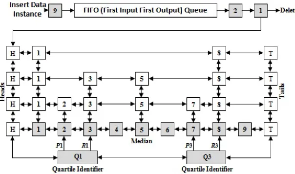
Figure 5.8 Real-time sorting of the feature data values using aSkipList. . . 72

Figure 5.9 An example of the update for the Quartile Identifiersfor Case 1 with a value inserted left ofQ1. . . 73

Figure 5.10 An example of the update for theQuartile Identifiersfor Case 1 with a value inserted between ofQ1andQ3. . . 74

Figure 5.11 An example of the update for theQuartile Identifiersfor Case 1 with a value inserted right ofQ3. . . 75

Figure 5.12 An example of the update for theQuartile Identifiersfor Case 2 with a value inserted left ofQ1. . . 76

(21)

value inserted between and . . . 76 Figure 5.14 An example of the update for theQuartile Identifiersfor Case 2 with a

value inserted right ofQ3. . . 77 Figure 5.15 An example of the update for theQuartile Identifiersfor Case 3 with a

value inserted left ofQ1. . . 78 Figure 5.16 An example of the update for theQuartile Identifiersfor Case 3 with a

value inserted betweenQ1andQ3. . . 78 Figure 5.17 An example of the update for theQuartile Identifiersfor Case 3 with a

value inserted right ofQ3. . . 79 Figure 5.18 The results ofSEAdata stream generator with a noise level of 0% using

Micro-Clusters for tracking features. . . 80 Figure 5.19 The results ofSEAdata stream generator with a noise level of 5% using

Micro-Clusters for tracking features. . . 82 Figure 5.23 The results of HyperPlanedata stream generator with a noise level of

0% using Micro-Clusters for tracking features. . . 82 Figure 5.24 The results of HyperPlanedata stream generator with a noise level of

35% using Micro-Clusters for tracking features. . . 84 Figure 5.28 The results ofRandom Tree data stream generator with a noise level of

(22)

35% using Micro-Clusters for tracking features. . . 87 Figure 5.33 The results ofSEAdata stream generator with a noise level of 0% using

Micro-Clusters for tracking features. . . 91 Figure 5.38 The results of HyperPlanedata stream generator with a noise level of

(23)

35% using Micro-Clusters for tracking features. . . 96 Figure 5.48 The results of CoverType dataset with 6 features (2 features swapped)

using Micro-Clusters for tracking features. . . 98 Figure 5.49 The results of CoverType dataset with 6 features (4 features swapped)

using Micro-Clusters for tracking features. . . 99 Figure 5.50 The results ofDiabetic Retinopathy Debrecendataset with 6 features (2

features swapped) using Micro-Clusters for tracking features. . . 99 Figure 5.51 The results ofDiabetic Retinopathy Debrecendataset with 6 features (4

features swapped) using Micro-Clusters for tracking features. . . 100 Figure 5.52 The results of Gesture Phase Segmentation dataset with 6 features (2

features swapped) using Micro-Clusters for tracking features. . . 100 Figure 5.53 The results of Gesture Phase Segmentation dataset with 6 features (4

features swapped) using Micro-Clusters for tracking features. . . 101 Figure 5.54 The results ofStatlog (Landsat Satellite) dataset with 6 features (2

fea-tures swapped) using Micro-Clusters for tracking feafea-tures. . . 101 Figure 5.55 The results ofStatlog (Landsat Satellite) dataset with 6 features (4

fea-tures swapped) using Micro-Clusters for tracking feafea-tures. . . 102 Figure 5.56 The results ofWaveform (with Noise)dataset with 6 features (2 features

swapped) using Micro-Clusters for tracking features. . . 102 Figure 5.57 The results ofWaveform (with Noise)dataset with 6 features (4 features

swapped) using Micro-Clusters for tracking features. . . 103 Figure 6.1 Process of feature selection in real-time. . . 108 Figure 6.2 An example of feature analysis, feature selection, and monitoring of

temporarily irrelevant features. Assumed Information Gains are indicated in italics, and actual Information Gain calculations are not in italics. . . 109 Figure 6.3 The results ofCoverTypedataset using Micro-Clusters for concept drift

(24)

for concept drift detection with/without real-time feature selection. . . 112 Figure 6.5 The results ofGesture Phase Segmentationdataset using Micro-Clusters

for concept drift detection with/without real-time feature selection. . . 113 Figure 6.6 The results of Statlog (Landsat Satellite) dataset using Micro-Clusters

for concept drift detection with/without real-time feature selection. . . 113 Figure 6.7 The results ofWaveform (with Noise) dataset using Micro-Clusters for

concept drift detection with/without real-time feature selection. . . 114 Figure 6.8 The results ofCoverTypedataset using Micro-Clusters for concept drift

detection with/without real-time feature selection. . . 115 Figure 6.9 The results ofDiabetic Retinopathy Debrecendataset using Micro-Clusters

for concept drift detection with/without real-time feature selection. . . 115 Figure 6.10 The results ofGesture Phase Segmentationdataset using Micro-Clusters

for concept drift detection with/without real-time feature selection. . . 116 Figure 6.11 The results of Statlog (Landsat Satellite) dataset using Micro-Clusters

for concept drift detection with/without real-time feature selection. . . 116 Figure 6.12 The results ofWaveform (with Noise) dataset using Micro-Clusters for

concept drift detection with/without real-time feature selection. . . 117 Figure 7.1 Workflow of Data Stream Mining for real-time feature extraction. . . . 124 Figure 7.2 Example of important and extreme limits of feature data’s range using

IQR. . . 125

Figure F.1 The actual values ofSplitandDeathrates ofSEAdata stream generator for drift detection. . . 162 Figure F.2 The actual values of Split and Death rates of HyperPlane data stream

generator for drift detection. . . 163 Figure F.3 The actual values of SplitandDeath rates ofRandom Tree data stream

generator for drift detection. . . 164 Figure F.4 The actual values of Split andDeathrates of CoverTypedataset with 6

features for drift detection. . . 164 Figure F.5 The actual values ofSplit andDeathrates ofDiabetic Retinopathy

(25)

dataset with 6 features for drift detection. . . 165 Figure F.7 The actual values ofSplit andDeathrates ofStatlog (Landsat Satellite)

dataset with 6 features for drift detection. . . 165 Figure F.8 The actual values of Split and Death rates of Waveform (with Noise)

dataset with 6 features for drift detection. . . 166

Figure G.1 The results of CoverType dataset with 6 features (2 features swapped) using Min-Max,LPF, andIQRfor minimising the effects of feature-bias, noise, and outliers. . . 168 Figure G.2 The results of CoverType dataset with 6 features (4 features swapped)

using Min-Max,LPF, andIQRfor minimising the effects of feature-bias, noise, and outliers. . . 168 Figure G.3 The results ofDiabetic Retinopathy Debrecendataset with 6 features (2

features swapped) using Min-Max,LPF, andIQRfor minimising the effects of feature-bias, noise, and outliers. . . 168 Figure G.4 The results ofDiabetic Retinopathy Debrecendataset with 6 features (4

features swapped) using Min-Max,LPF, andIQRfor minimising the effects of feature-bias, noise, and outliers. . . 169 Figure G.5 The results of Gesture Phase Segmentation dataset with 6 features (2

features swapped) using Min-Max,LPF, andIQRfor minimising the effects of feature-bias, noise, and outliers. . . 169 Figure G.6 The results of Gesture Phase Segmentation dataset with 6 features (4

features swapped) using Min-Max,LPF, andIQRfor minimising the effects of feature-bias, noise, and outliers. . . 169 Figure G.7 The results ofStatlog (Landsat Satellite) dataset with 6 features (2

fea-tures swapped) using Min-Max, LPF, and IQR for minimising the effects of feature-bias, noise, and outliers. . . 170 Figure G.8 The results ofStatlog (Landsat Satellite) dataset with 6 features (4

fea-tures swapped) using Min-Max, LPF, and IQR for minimising the effects of feature-bias, noise, and outliers. . . 170

(26)

swapped) using Min-Max, , and for minimising the effects of feature-bias, noise, and outliers. . . 170 Figure G.10 The results ofWaveform (with Noise)dataset with 6 features (4 features

swapped) using Min-Max,LPF, andIQRfor minimising the effects of feature-bias, noise, and outliers. . . 171 Figure H.1 The results ofSEAdata stream generator using Micro-ClusterPercentage

DifferenceofSplitandDeathrates for drift detection. . . 173 Figure H.2 The results of HyperPlane data stream generator using Micro-Cluster

Percentage DifferenceofSplitandDeathrates for drift detection. . . 173 Figure H.3 The results ofRandom Tree data stream generator using Micro-Cluster

Percentage DifferenceofSplitandDeathrates for drift detection. . . 174 Figure H.4 The results ofSEAdata stream generator using Micro-Clusters for

track-ing features. . . 176 Figure H.5 The results of HyperPlanedata stream generator using Micro-Clusters

for tracking features. . . 176 Figure H.6 The results ofRandom Treedata stream generator using Micro-Clusters

for tracking features. . . 177 Figure I.1 The results ofSEAdata stream generator using Micro-ClusterPercentage

DifferenceofSplitandDeathrates for drift detection. . . 180 Figure I.2 The results of HyperPlane data stream generator using Micro-Cluster

Percentage DifferenceofSplitandDeathrates for drift detection. . . 180 Figure I.3 The results ofRandom Tree data stream generator using Micro-Cluster

Percentage DifferenceofSplitandDeathrates for drift detection. . . 180 Figure I.4 The results ofSEAdata stream generator using Micro-Clusters for

track-ing features. . . 182 Figure I.5 The results of HyperPlanedata stream generator using Micro-Clusters

for tracking features. . . 183 Figure I.6 The results ofRandom Treedata stream generator using Micro-Clusters

(27)

ADWIN ADaptive sliding WINdow

CUSUM CUmulative SUM

DSM Data Stream Mining

DDM Drift Detection Method EDDM Early Drift Detection Method

EWMA Exponential Weighted Moving Average FIFO First In First Out

FS Feature Selection

IQR Interquartile Range

LPF Low Pass Filter

MC-NN Micro-Cluster Nearest Neighbour

Min-Max Minimum-Maximum

MOA Massive Online Analysis

(28)

Introduction

This chapter presents the research background and discusses the importance of developing dy-namic feature selection techniques in combination with real-time concept drift detection meth-ods. There is an apparent lack of techniques that can do both in the field of data stream mining. The discussion introduces the main research areas and factors that have significantly affected the Data Stream Mining algorithms. Then the research problem is discussed under academic and methodological perspectives. Next, the scope of research, motivations for research, the re-search objectives, and methodology of rere-search are presented. The chapter is concluded with an outline of the thesis and summary of the chapter.

1.1

Background and Problem Statement of the Research

Velocity in Big Data Analytics (Ebbers et al., 2013) refers to data that is generated at ultra-high speed and is live-streamed (i.e., a data stream) whereupon the processing and storing of it in real-time constitutes significant challenges to current computational capabilities in com-puting systems (Babcock et al., 2002; Gaber et al., 2005). Thus, Data Stream Mining (DSM) has been developed. Useful information from a data stream can be extracted using DSM. In other words, DSM is the analysis of unbounded and sequential data instances that are unseen, generated, labelled automatically, and arrive with a highVelocityin real-time. Thus in DSM, algorithms need to be capable of learning over a single-pass through the training data (Gaber et al., 2005). The general area of DSM covered by this research is to solve problems associated with lack of pre-processing techniques in the context of data stream classification, which is the prediction of class labels of new instances in the data stream in real-time. Potential applications

(29)

that need real-time data stream classification techniques are for data streams in the chemical process industry (Kadlec et al., 2009), intrusion detection in telecommunications (Jadhav et al., 2013), credit card fraud detection (Salazar et al., 2012), Internet traffic management and weblog analysis (Gama, 2010), sensor networks, etc.

Data stream classification need not only be able to incrementally learn but also be able to adapt to concept drift over a statistical time window using the most recent data from the stream (Gama and Gaber, 2007; Bifet, 2009; Hoens et al., 2012).

A concept drift occurs if the pattern encoded in the data stream changes. DSM has devel-oped various real-time versions of established predictive data mining algorithms that adapt to concept drift and keep the model accurate over time, such as CVFDT (Hulten et al., 2001) and G-eRules (Le et al., 2017). The benefit of classifier independent concept drift detection meth-ods is that they give information about the dynamics of data generation (Gama et al., 2014). Common drift detection methods are for example ADaptive sliding WINdow (ADWIN) (Bifet and Gavalda, 2007), Drift Detection Method (DDM) (Gama et al., 2004) and the Early Drift Detection Method (EDDM) (Baena-Garcıa et al., 2006).

However, these methods are suffering from feature-bias, outliers, and noise (Dongre and Malik, 2014; Brzezinski and Stefanowski, 2014; Frías-Blanco et al., 2015). In addition, no drift detection method devised to-date can provide potentially highly valuable insights as to which features are involved in the concept drift. For example, if a feature is contributing to a concept drift, it can be assumed that the feature may have become either more or less relevant to the cur-rent concept. This has inspired the development of a real-time feature tracking method based on feature contribution information for the purpose of feature selection to identify features that have become relevant or irrelevant due to concept drift. Thus, in this research, a technique for detecting causality of drifts, and providing the feature contribution information over a statistical time window of data instances which is kept in short-term memory in real-time has been devel-oped. Based on this, tracking features and identifying the relevant features of a classifier for the purpose of feature selection in real-time have also been developed.

Feature contribution information in this research is formulated or represented asVelocity and the spread of a feature’s data. Velocityis the rate of change of features centroidsover a statistical time window (i.e., the difference between the current and previous centroidof each feature). Regarding feature selection, common feature selection methods are for example Linear Discriminant Analysis (LDA), Canonical Correlation Analysis (CCA), Multi-View CCA, and

(30)

Principal Component Analysis (PCA) (Ahsan and Essa, 2014; Lee et al., 2015). These methods can be applied to a sample of the data stream before commencing the training and adaptation of a data stream classifier. However, this would not account for changes in the relevance of features over time for the classification task at hand due to concept drift which can only be dealt with by re-running the above methods to update the feature rankings to accommodate any drifts. However, this can potentially be an expensive procedure especially if there are many dimensions in the data, hence the rationale for a single-pass method requiring the re-evaluation of only the features whose classification relevance has changed since the last pass.

This research, therefore, describes a concept drift detection method for data stream classifi-cation algorithms with the feature tracking information feedforward capability linking features to concept drifts over a statistical time window for feature selection purposes. The method only needs to examine features that have potentially changed their relevance and only when there is an indication that the relevance of a feature may have changed. The developed method can be used with any learning algorithm either as a real-time wrapper or a batch classifier or realised inside a real-time adaptive classifier (Domingos and Hulten, 2000).

1.2

Scope of Research

This study aims to improve the DSM classification algorithms in terms of the classification tasks’ accuracy through enabling real-time concept drift detection with automatic dimensional-ity reduction in specific feature selection. In this study, the focus is given more on both detecting drifts and feature selection with adaptive summaries of the data and class distributions with con-tinuous features, known as Micro-Clusters (Zhang et al., 1996; Aggarwal et al., 2003; Tennant et al., 2017). Micro-Clusters group the data points according to their similarities of charac-teristics using a distance function such as Euclidean distance. Feature extraction is out of the scope of this study. However, it can be developed by further developing this research regarding identifying and detecting redundant features. Feature-bias, outliers and noise may influence DSM techniques (i.e., clustering and classification). Thus, robustness handling or minimising the effect of feature-bias, outliers, and noise has been taken into consideration in this research study. In addition, the in this research developed technique (i.e., a pre-processing technique) is independent of the data mining algorithm, i.e., this is also out of the scope of this study. However, a classifier can be developed by embedding the developed technique to identify and

(31)

detecting the best feature subset in real-time.

1.3

Motivations for Research

This section discusses the main factors that motivate the research undertaken and investigated which is the problem of real-time feature selection. Nowadays the focus of DSM lies in the development of data mining algorithms rather than on pre-processing techniques. The feature selection previously proposed are typically applied before a classifier is introduced as they are not designed for data streams as they do not take into consideration that the relevance of a feature for a classification task may change over time. To the best of the author knowledge, at present, there are no developments for truly real-time feature selection in a streaming setting. This is important as features may potentially change their relevance for data mining tasks based on specific measures of relevance such as Information Gain. Thus the three objectives of this research were to develop a real-time pre-processing technique that can detect a concept drift, identify features that were involved in concept drift and thus potentially change their relevance, and build a real-time feature selection method.

1.4

Research Objectives

The objective of this work is to highlight the problems associated with lack of pre-processing techniques to a DSM algorithm in real-time. This will improve the accuracy of the classification task of a data stream classifier.

1. To develop and comparatively evaluate a method to identify a drift point (i.e., concept drift) through tracking the significant changes in the statistical summaries in real-time, 2. To develop and evaluate a method to detect causality of drifts (which is identified by

the developed method in Objective 1 above) through providing the historical statistics of each feature for identifying which features were involved in drifting over a statistical time window in real-time,

3. To develop a method to continuously analyse the historical statistics provided by the developed method in Objective 2 above with the purpose of selecting the relevant features for adaptive data stream classifier (i.e., dynamic adjustment feature selection in real-time).

(32)

1.5

Methodology of Research

This section illustrates the methodology of this research study which can be outlined as follows: literature review stage, design stage of the developed framework and methods, implementation stage, and evaluation stage.

1.5.1

Literature Review Stage

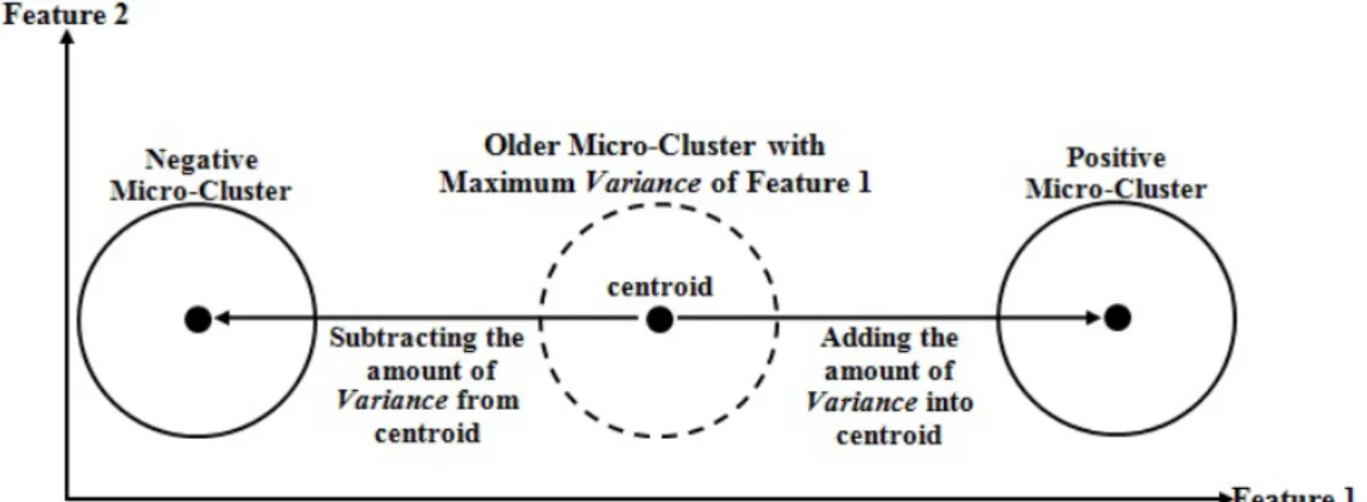
In this stage, the related concepts to the research study are reviewed which are concept drift, feature selection, data stream classification, and data stream clustering. The review includes the concepts related to the various methods and algorithms previously proposed. The review also identifies initially what needs to be improved in order to make effective data stream pre-processing technique in specific real-time feature selection method. This method does not need to examine the entire feature space. This can be achieved by applying concept drift detection method in combination with feature tracking method, and providing the statistical summaries feedforward capability linking features to concept drifts over a statistical time window. In addition, in this stage, the original MC-NN algorithm which was developed by (Tennant et al., 2017) is summarised as it has been identified as a promising classification approach. MC-NN has originally been developed for predictive data stream analytics using Micro-Clusters which are able to adapt to unexpected changes on the stream. However, this research is not concerned with the classification capabilities of MC-NN but in the behaviour of its underlying model during concept drift. Moving in different directions (i.e., a direction represents a feature) is the original purpose of a Micro-Cluster in order to adapt to concept drift and maintain an accurate model. This has inspired the idea of this research study (i.e., tracking the behaviour of Micro-Clusters) to be modified to detect concept drift, causality of concept drift, and enabling continuous feature selection. Figure 1.1 shows an example of Micro-Clusters with two features (i.e., two directions). A Micro-Cluster can move in one or more directions.

(33)

Figure 1.1: An example of Micro-Clusters with two features.

The review also includes an evaluation which aims to show which method or algorithm previously proposed is capable of handling both concept drift detection and dynamic feature selection, as well as providing the statistical summaries with single-pass processing through streaming data in real-time.

1.5.2

Design a Framework of the Developed Methods Stage

In this stage, three developed methods are identified and designed. A method to identify a drift point (i.e., concept drift) in real-time. A method for detecting causality of drifts providing the historical statistics (i.e., Velocity and the spread of a feature’s data) of tracked features over a statistical time window in real-time. A method for identifying irrelevant features which are involved in drifting detected in the aforementioned methods through analysing the tracked fea-tures and applying dynamic adjustment feature selection in real-time. The developed methods are embedded in a proposed framework which consists of minimising the effect of feature-bias, minimising the effect of noise, drift detection with tracking the involved features, and feature se-lection. The central components of this framework are drift detection with tracking the involved features and feature selection. The MC-NN approach that has been reviewed in Stage 1.5.1 is used in the central components which detect drifts and provide statistical information for the purpose of tracking which features were involved. The aims and functions of each component

(34)

are determined, as well as the input and output of each component are identified (Chapters 4, 5, and 6), so that a clear interaction and flow between the components are achieved. Figure 1.2 illustrates the proposed framework.

Figure 1.2: The framework of the developed methods.

The major tasks of the proposed framework are to detect a concept drift with the feature tracking information feedforward capability linking features to concept drifts over a statistical time window for feature selection purposes. This method does not need to examine the entire feature space using the adaptive Micro-Clusters.

1.5.3

Implementation Stage

The proposed framework consists of the developed methods that have been designed in stage 1.5.2 is implemented and realised in the Java-based Massive Online Analysis (MOA) framework (Bifet et al., 2010).

Two types of data were used, artificial data stream generators from the MOA framework and real datasets. The reason for using artificial datasets is because MOAs data stream gener-ators enable the introduction of different kinds of concept drift deliberately and thus allow this research to evaluate against a ground truth regarding concept drift.

(35)

1.5.4

Evaluation Stage

In this stage, the performance of the developed method for concept drift detection is evaluated with respect totrue positivedetections of known ground truth concept drifts in comparison with the competing alternative concept drift detection methods. Regarding the performance of the developed method for feature tracking is evaluated with respect to true positive detections of features involved in drifting. Whereas, the performance of the developed method for real-time feature selection is evaluated with respect to the accuracy of a data stream classifier achieved using the developed method compared with not using the method. Where the data stream clas-sification method chosen was Hoeffding Tree as well as incremental NaiveBayes.

1.6

Organisation of Thesis

The rest of this thesis is organised as follows. Chapter 2 analyses literature about the fun-damental meaning of concept drift, feature selection, data stream classification, data stream clustering, and Micro-Clusters.

Chapter 3presents the structure of Micro-Cluster Nearest Neighbour (MC-NN) algorithm developed by (Tennant et al., 2017). MC-NN has originally been developed for predictive data stream analytics and is modified in this research to serve as the basis for the methods developed.

Chapter 4presents the developed method for detecting drifts which is based on the Micro-Cluster structure of the MC-NN classifier presented in Chapter 3. A research paper has been published which consists of the developed method for drift detection with a preliminary result which shows that the developed method is capable of detecting a concept drift but also delivers an indication which features are involved.

• Title: Towards Online Concept Drift Detection with Feature Selection for data stream classification,

• Authors: Mahmood Shakir Hammoodi, Frederic Stahl, and Mark Tennant,

• Year: 2016,

• Publisher: IOS Press (ECAI).

Chapter 5presents the developed method for tracking the features involved in drifting by monitoring statistical information provided by adaptive Micro-Clusters. A research paper has

(36)

been published which consists of the developed method for tracking feature in combination with drift detection as well as preliminary results which show that the developed methods are capable of detecting a concept drift and delivering an indication which features are involved compared with alternative concept drift detection methods.

• Title: Towards Real-Time Feature Tracking Technique using Adaptive Micro-Clusters,

• Authors: Mahmood Shakir Hammoodi, Frederic Stahl, Mark Tennant, and Atta Badii,

• Year: 2017,

• Publisher: BCS Specialist Group on Artificial Intelligence.

Chapter 6 presents the developed method for dynamic feature selection in real-time. A research paper has been published which consists of the holistic work of this research study, as well as an in-depth evaluation of the developed methods which are drift detection method, fea-ture tracking method, and real-time feafea-ture selection method with respect to different artificial and real datasets.

• Title: Real-Time Feature Selection Technique with Concept Drift Detection using Adap-tive Micro-Clusters for Data Stream Mining,

• Authors: Mahmood Shakir Hammoodi, Frederic Stahl, and Atta Badii,

• Year: 2018,

• Publisher: Elsevier on Knowledge-Based Systems.

Conclusion and future works as guidelines for further research that can be added to the work drawn from this thesis are summarised inChapter 7.

1.7

Summary

This chapter explains the background of this thesis. It discussed the main factors that have sig-nificantly affected the DSM algorithms. This study is motivated by the apparent lack of research in real-time feature selection in a streaming setting. In addition, it is argued that the DSM clas-sification algorithms can be improved in terms of accuracy of clasclas-sification task by applying a real-time pre-processing technique which detects drifts and selects relevant features for the

(37)

classifier dynamically. Some backgrounds and concepts of concept drift, feature selection, data stream classification, and data stream clustering will be explained in greater detail in the next chapter.

(38)

Background and Literature Review

In Chapter 1, the aims and objectives were highlighted and described which led to defining the research problem. Chapter 2 presents the background and literature review that formulates the foundation on which this research is based. This chapter discusses the concepts of data stream pre-processing technique, concept drift, feature selection, data stream classification, and data stream clustering. The chapter also reviews related and relevant methods and algorithms. This identifies initially what needs to be improved in order to make an effective data stream pre-processing technique in specific real-time feature selection method. This can be achieved by applying concept drift detection method in combination with feature tracking method. This could be used with any learning algorithm either as a real-time wrapper or a batch classifier or realised inside a real-time adaptive classifier (Domingos and Hulten, 2000). The chapter is organised as follows. In Section 2.1, Data Stream Mining (DSM) is explained. Section 2.2 gives an overview of general data stream processing techniques. The data stream pre-processing techniques are presented in Section 2.3. Adaptive DSM algorithms are discussed in Section 2.4. Section 2.5 analyses the reported methods and algorithms in this chapter with respect to the research objectives. Section 2.6 summarises this chapter.

2.1

Data Stream Mining (DSM)

DSM is the analysis of unbounded and sequential data instances that are unseen and arrive with a highVelocity in real-time. In other words, the stream arrives online (i.e., instance by instance) and there is no control over the order in which data instances arrive either within a data stream or across data streams. Once an instance from a data stream has been handled, it can

(39)

not be retrieved as it is discarded (Gama and Gaber, 2007). The main characteristics of streams include susceptibility to concept drift which is a problem and an area of research as well as handling dimensionality, i.e., features may become irrelevant to a classifier in general over time (Brzezi´nski, 2010; Ahsan and Essa, 2014; PhridviRaj and GuruRao, 2014). This implies the following requirements on data mining algorithms learning from data streams in real-time:

1. One data instance at a time is examined and processed.

2. A limited amount of memory is required. 3. Predict at any time and demand.

4. Adapt to concept drift in case of changes in the patterns encoded in the data stream.

5. Irrelevant features to a classifier have to be discarded and monitored in real-time, i.e., feature selection needs to be applied dynamically over time.

Next in Section 2.1.1, a general overview of workflow of DSM will be presented.

2.1.1

Workflow of DSM

This section presents the workflow of DSM in terms of feature selection and concept drift detection. Figure 2.1 shows the typical workflow of feature selection and concept drift detection in predictive data stream analysis. The best candidate features from given training data are typically identified and selected by feature selection. The existing feature selection methods need to be applied in advance (i.e., offline) (see Section 2.3.5). A classifier is then introduced to build a model using the selected features which may change over time. Thus, dynamic feature selection is required. Whereas, concept drift detection methods are either applied offline or unable to handle unexpected changes in data (see Section 2.3.4). In addition, in these methods, the features involved in drifting are not identified i.e., the features that cause the drift.

(40)

Thus, adaptive and computationally efficient algorithms are required to analyse streaming data in real-time in terms of concept drift detection with dynamic feature selection which does not to examine the entire feature space, as shown in Figure 2.2. Where Test and Train refer to Test-Then-Train or Prequential. Each individual data instance is used to test the model before it is used for training over time stamps (Bifet and Frank, 2010). Where a time stamp is the current time of a data instance that is used to test and train the model. Examining unexpected change in data (i.e., concept drift) is applied over a statistical windowing approach with a fixed size (i.e., time window with 1000 data instances as an example). Where a time window is a set of time stamps. Hence, features which were involved in drifting are discarded using feature selection (i.e., irrelevant to a classifier). However, the discarded features are ranked and evaluated over time to be selected as relevant to a classifier using feature selection (i.e., dynamic feature selection). Based on this the accuracy of a classification task of a data stream classifier will be improved.

Figure 2.2: Workflow of Data Stream Mining.

Next in Section 2.1.2, a general overview of concept drift will be presented as its the under-lying motivation of this research study.

2.1.2

Concept Drift

A concept drift occurs if the pattern encoded in the data stream changes over time. The gathered data changes or shifts after a stability period. Identifying a drift point as distinct from noise or outlier is the first and most challenging task for drift detection algorithms (Bose et al., 2014; Gama et al., 2014). Thus analytics algorithms need to adapt. This issue of concept drift needs to be considered in order to mine relevant data with appropriate accuracy. At least four types

(41)

of drift can be identified; gradual, sudden, recurring, and incremental, as well as noise and outliers which may occur in the data stream (Aggarwal and Yu, 2001; Brzezi´nski, 2010; Bose et al., 2014; Gama et al., 2014). The different types of concept drift are depicted in Figure 2.3.

Figure 2.3: Types of concept drifts.

Regarding Figure 2.3gradual concept driftrefers to a present concept progressively chang-ing into a new concept within a short period of time whereas sudden concept drift refers to the instant replacement of the current concept by a new concept. A recurring concept drift refers to a previous concept re-appearing at a later stage, this can be both sudden or gradual. An incremental concept drift refers to a constantly evolving concept and these are generally hard to detect. Outliers and noise are not concept drifts. Often it is challenging for concept drift detection methods to distinguish noise and outliers from real concept drift (Brzezinski and Stefanowski, 2014; Gama et al., 2014).

Next in Section 2.2, an overview of general data stream processing techniques is presented, and in Section 2.3 DSM in terms of handling and adapting to concept drift is presented in greater detail.

2.2

Overview of General Data Stream Processing Techniques

This section presents the techniques which are frequently used for processing data streams in terms of handling and adapting to concept drift which are statistical summaries with single-pass processing, windowing approaches, and adaptive algorithms.

(42)

2.2.1

Statistical Summaries with Single-Pass Processing

In data stream processing, handling and adapting to unexpected changes (i.e., concept drift) can be achieved by providing and performing statistical summaries over the most recent data instances, and over summarised versions of the old instances. This is called online-offline pro-cessing (Ren and Ma, 2009). However, a data stream may be unbounded and arrive continuously at a highVelocityover time. This poses challenges as multiple scans over the stream is not pos-sible or infeapos-sible in real-time. Only single-pass processing through the data is required. This will be highlighted in more detail in Section 2.4.

2.2.2

Windowing Approaches

In data streams, the most recent information from the stream is likely to represent the new changes in the data distribution which can be used for the purpose of analysis of concept drift. Windowing approaches have been used to deal with concept drift using only recent data instead of the whole data stream (Gama and Gaber, 2007; Bifet, 2009; Hoens et al., 2012). There are three commonly used models in data streams which aresliding windows,damped windows, and landmark windows(Silva et al., 2013). In thesliding windows, only the most recent information from the data stream is kept in a data structure (i.e., a first in, first out (FIFO) queue) whose size can be fixed or identified in advance. The first value added to the window will be the first one to be removed. The damped windowsprovide the most recent information by associating weights with instances from the data stream. The weights of the instances decrease with time, and more recent instances receive a higher weight than older instances. Regarding thelandmark windows, the whole data stream is divided into chunks (i.e., windows) to be handled as updating units. When a new landmark arrives, all instances saved into the window are deleted, and the new instances from the current landmark are saved in the window until a new landmark arrives. However, in data stream monitoring or analytics, thesliding windowis frequently used as it is keeping the most recent information of the stream (Zhu and Shasha, 2003; Lakshmi and Reddy, 2015).

2.2.3

Adaptive Learning Algorithms

Adaptive learning algorithms often need to be operated in environments that are changing rapidly or unexpectedly over time. If the data generating process is unstable, the underlying

(43)

concept may be drifting over time. The ability to incorporate new data is a desirable property of these algorithms and is considered as a natural extension for the incremental learning algorithms (Gama et al., 2014). Adaptive DSM algorithms will be highlighted in more detail in Sections 2.4.1 and 2.4.2.

2.3

Data Stream Pre-Processing Techniques

In general, when applying data mining algorithms, low-quality data will lead to low-quality data mining models. Hence, pre-processing techniques have to be taken into consideration in order to guarantee a quality of the models, and it can often have a significant effect on generalisation performance of a machine learning algorithm (Gaber et al., 2005; Han et al., 2011). Several types of problems can be resolved by applying a data stream pre-processing technique which consists of minimising the effect of feature-bias, noise, and outliers as well as feature subset selection which is the process of identifying and removing irrelevant features which may not be related to the target concept (Hu, 2003; Kotsiantis et al., 2006; Yan et al., 2006; Davis and Clark, 2011). Moreover, in real-world data, the gathered data often changes or shifts after a minimum stability period. A concept drift detection method needs to be considered and taken into consideration in the pre-processing technique in order to mine relevant data with appropriate accuracy (Ramírez-Gallego et al., 2017). This will be highlighted in the next sections.

2.3.1

Minimising the Effect of Feature-Bias

Normalisation is applied to fit the data (i.e., each feature of a new training instance) to be almost distributed in a pre-defined boundary such as [0,100]. Normalisationis used to avoid feature-bias which can potentially lead to mis-classifications as the relevant relations between target class labels and features are considered by the classifier to be more or less important than they actually are (Fan and Davidson, 2006; Pelayo Ramirez, 2011).

Three frequently used types ofNormalisationare i.e. Min-Max (see Equation 2.1), Decimal Scaling (see Equation 2.2), and Z-Score (see Equation 2.3) (Ogasawara et al., 2010).

x=

current value−minx maxx−minx

(44)

x= x

(10d₎ (2.2)

x= x−µ

σ (2.3)

xis a feature value of the new data instance. Min-Max is a simpleNormalisationtechnique to fit the data in a pre-defined boundary with a minrange(default 0) and a maxrange(default 100). Decimal Scaling moves the decimal point of a feature valuexdepending on its maximum absolute value. Whereby d equals to MAX(|y|)<1 (i.e., the smallest value of a featurey). Lastly, Z-Score normalises a feature valuexaccording to its corresponding meanµand standard

deviationσ feature values. However, Decimal Scaling and Z-Score rely on theσ and theµ and

thus require the buffering of data beforeNormalisationcan be applied. Whereas, minxand max xof Min-Max can be re-initialised over time stamps as the buffering of data is not required. It does not rely on theσ and theµ as it can be updated instance by instance. In addition, Liu et al.

(2011) and Patro and Sahu (2015) stated that in Min-Max, a complex calculation is not required, and it has better performance in terms ofNormalisationin comparison with the aforementioned techniques. This has inspired the idea of applying Min-Max in real-time in this research study.

2.3.2

Minimising the Effect of Noise

Noise is defined as a random error or Variance in a measured variable, or randomly occur-ring errors (i.e., data inconsistency, out-of-range values) (Zhang, 2008). In machine learning algorithms, mis-classification could happen as noise is misleading relationships between the features and the class labels (Hickey, 1996; Zhang, 2008). Thus, minimising the effect of noise is required. There are some techniques proposed for the purpose of filtering such as the Kalman filter and Grid-based filter (Bhowmik and Roy, 2007) which require buffering of data before filtering (Arulampalam et al., 2002). In the Kalman filter, the posterior density at every time is Gaussian which is parameterized in terms of µ and Covariance. Whereas, in Grid-based

tech-nique, the optimal recursion of the filtered density is provided when the state space is discrete and consists of all relevant information required to describe the data. Where, the state space refers to the Euclidean space in which the variables (i.e., the number of inputs, outputs, and states) on the axes are the state variables which can be expressed as vectors. State variables are variables whose values developed gradually through time. However, there is another technique

(45)

proposed called Low Pass Filter (LPF) (Rosenholtz and Zakhor, 1991; Schall et al., 2005). It does not rely on the σ and the µ as it can be updated instance by instance. This has inspired

the idea of applyingLPF in real-time in this research study. LPF is a filter that passes signals (i.e., the Velocity of a feature) with a frequency lower than a certain cut-off frequency α and

attenuates signals with frequencies higher than the cut-off frequency using Equation 2.4.

new f ilter[x] =α∗new value[x] + (1−α)∗old f ilter[x] (2.4)

x is a feature value of the new data instance. new f ilter[x] and old f ilter[x] can be re-initialised over time stamps as the buffering of data is not required.

2.3.3

Minimising the effect of Outliers

Outliers are data stream instances outside the expected range of values. In other words, it is an observation that is numerically distant from the rest of the data (Zhang, 2008). Hence, it has a significant effect on statistical analysis (Zhang, 2008). Thus, minimising the effect of outliers is needed. There are some techniques proposed for the purpose of outliers detection such as Distance-based and Density-based (Knox and Ng, 1998; Knorr and Ng, 1999; Ramaswamy et al., 2000; Breunig et al., 2000) which are generally unable to deal with the curse of high dimensionality (Aggarwal and Yu, 2005). However, there is another technique proposed to minimise the effect of outliers which is called Inter Quartile Range (IQR). It is considered a more robust method to outliers (Leys et