On the Accuracy and Properties of Recent Macroeconomic Forecasts

ON THE ACCURACY AND PROPERTIES OF RECENT ACROECONOIC FORECASTS

Victor Zarnowitz*

University

of Chicago

and

National Bureau of Econoiic Research

Working Paper No. 229

NAIIONAL BUREAU OF ECONOMIC RESEARCH, INC.

261 Madison Avenue New York, N.Y. 10016

Revised February 1978

Preliminary; Not for Quotation

NBER working papers are distributed informally and in limited number for comments only. They should not be quoted without written permission.

This report has not undergone the review accorded official NBER publications; in particular, it has not yet been submitted

for approval by the Board of Directors.

NOTE:

This

is an abbreviated version of a report on work in progress supported by grants from the National Science Foundation and the Earhart Foundation to the National

Bureau of Economic flesearch.

*1 am grateful to Dennis Bushe, Thomas TZutzen, and oert Osterlund for assistance with research and preparation of

ON THE ACCURACY AND PROPERTIES OF

RECENT MACROECONOMIC FO!ECASTS

Abstract

The aim of this study is to contribute to the measurement and analysis

of errors in economists' predictions of changes in aggregate income, output,

and. the prIce level. n11

sample

studies of forecasts can be instructive,

it their limitations must be recognized. Compilation of consistent forecast

records extending over longer periods of tine is necessary to establish a

reasonably reliable base for assessments of forecasting behavior and. perfor—

mance. Thus the historical record of post—World War II forecasts assembled

in the 1960's by the NB is here extended and updated.

The end—of—year predictions of annual percentage changes in GNP earn

good marks for overall accuracy when judged according to realistic rather

than ideal standards. Moreover, they are found to have improved significantly

in the period since the early l96O s compared with the previous years after

World War II.

The corresponding predictions for GNP in constant dollars (real

growth) and the GNP implicit price index (inflation) are considerably poorer.

The former suffer fran large turning point errors, the latter from large

underestimation errors. Indeed, forecasts of inflation are not much better

than projections of the most recently observed inflation rates, and they lag

behind the actual rates much like such projections. But the errors in

forecasts of real growth are negatively correlated with the errors in forecasts

Forecasts

for the year as a whole can

be

_{satisfactory when based}

on

a

good record for the first two

_quarters;

they tend.

_{to be more accurate than} forecasts

with longer spans. An exaiination of the recent multiperiod

pre-dictions fr veU—kiown econometric models and. business outlook

surveys shov

that

the errors for real growth and inflation cumulated rapid.ly beyond. the

spans.of 2 to 1 cpiarters. Previous studies have shon the cumulation to be

as

a

rule less than proportional to the increase in the span, but in the

period of recession and recovery 1973—75 the build—up of

errors was much greater.

Again the nominal GNP forecasts benefitted from offsetting errors

as the rise in

prices was heavily underestimated and

the downturn in real

activity was missed. Forecasters were generally unprepared for the concurrence

of accelerating inflation and slowing, then declining output rates: they

optimistically

(and. probably also from a lingering faith in a simple Phillips trade-off) kept anticipating less inflation and

more

_growth.

At

the present time, the predictive value of detailed multiperiod

forecasts reaching out further than a few quarters ahead must be rather

heavily discounted. No doubt, in periods less turbulent than the recent

past the longer forecasts can be considerably more accurate, but thiz fair—

weather

argument is not very persuasive or helpful.

Victor Zarnowitz

Graduate School of !3usiness

University of Chicago

Chicago, Illinois 60637

312/753—3615

Victor Zarnowitz

I.

On Some Uses and

limitations

of Forecast Data

How

and how well economists forecast, and how much their predictions

•

help or hurt public and. private decision mdcing, are matters that

ought

to

receive much attention of the profession. This is so ot only because of

their direct

interest to the authors, users, and critics of the forecasts,

but

also because

of

their intrinsic

but less evident academic interest. hat

is

the practical applicability of economic analysis in this critical area?

l4hat

is the quality

of

foresight and counsel that can

be expected of

respon-sible economists?

These are

broad

questions which

are not

easy to answer,

but they

are basic

and.

surely deserve

to be tackled. This

requires

that we

systematically confront forecasts as indications of

how economists

cx ante thought

events

are likely

to

un.fold

with

cx post knowledge of what actually

did.

happen and how.

The aims, from tie

least

to t.e

most

ambitious, are

(1)

to

measure forecast errors, (2) to explain them, and (3)

to

learn how to

reduce them in the future.

Success

in forecasting may be occasional and. fortuitous or

intuitive,

but

progress in. forecasting, to the extent it is possible, can only come from

advances of science, not art or chance. It presupposes

that

su.fficiently

important and persistent

regularities in economic processes and

relationships

ed.st

and

be properly identified and. used. Learning processes are

involved,

which

can be

time-consuming

arid, discontinuous,

reflecting in. part

the shifts

and

discontinuities in

the econrmc change itself,

in

part the inadequacies

of

measurement

and

analysis.

Data

on economic forecasts generally cover short tine periods. Iørlg

tine series on

consistent

predictions simply do not exist. Few if

any

that

matter (source,

target,

timing,

assumptions,

data, models,

and

methods used),

so that it

is often d.ifficult to determine what constitutes a suitable

"sample"

of forecasts of a given type. Moreover, few forecasters leave their

models and. techniq.ues unchanged for long as they seek inprovements and try to

adapt to new developments in the economy. Hence, a particular forecaster's

past record is often a hi.ly uncertain basis for inferences how he will

perform in the future.

Even

more hazardous, if not irresponsible, are attempts to grade

fore-casters on the evidence of how well they predicted change in. a particular

short period, say, a year or a few years. C].early, on any individual occasion

sce forecasters will, be ahead of others by sheer chance or for some

idio-syncratic reasons. Strong evidence of significant and stable differences over

time would be required to rank the forecasting individuals, groups, or models

with a modicum of confidence, and, such evidence is essentially lacking

(Zarnowitz, 1967, 1971; Christ; McNees, 1975).

The proliferation in recent years of mu.ltiperiod. quarterly

macro-forecastz offers no substitute for long historical series. These are rich

data

containing much interesting material that certainly deserves to be

care-fully recorded and analyzed. However, such forecasts, and. so their errors,

tend. to be internally correlated in at least two ways: (a) serially, Within

each

sequence made from a given base period. and (b) across the successive

sequences, which overlap and thus refer partially to the sane target period.

Each multiperiod forecast is a joint product of the common infornation,

technique, and juderit used, and each depends on previo..s forecasts of which

it is to some extent a revision. Thus, errors in the data, models, procedures,

and jtidents, autocorrelated disturbances, and certain types of distributed

multi-period

forecasts. The

resulting

complex correlation structures resist

estima-tion,

given the small samples of comparable predictions from any giverx source.

Consequently, measures of average accuracy, bias, etc., calcui.ated

from such

samples are difficult to interpret from the viewpoint of

statistical inference

(Spivey and. Wrobleski).

Two conclusions are surely

valid.. First,

small-sample studies cf

fore-casts are still needed and can be instructive, but their llmi tations must be

recognized. Second, it is necessary to compile and. examine forecast records

extending as far back in time as possible, so as to gain information, take a

lcnger view of forecasting behavior and. performance, and place the short

records of recent predictions in a proper perspective. Historical data on•

post-World. War II forecasts assembled in the 1960's by the National Bureau.

of Economic Research provide a good base here, which I was able to partially

extend and update. Some pre1cm1nary results for annual forecasts of three

variables

are

reported below.

II.

The Record of Annual GNP Forecasts Since 1914.7

In the

early post-World

War

II

period, most forecasts were made near the end of the

calendar

year

for

the next year

and

most referred to GNP

in

current

dollars. The evidence

we have on such forecasts goes back to 1914.7

but is quite fragmentary for the late 1914O's and early 1950's.

The period of transition from the

war

economy witnessed the largest

errors on record in the

GNP

forecasts.

Even after the 1914.5-14.6 predictions

were

shown to have greatly underestimated the then prev±ling levels ci' economic

activity (Klein, 1914.6), expectations of a business slump stubbornly persisted.

One =a].l, reputable group of private forecasters came up with an

average

prediction for 1914.7 of a 6

percent

decline in G?, whereas the actual change

fractional

decline but GNP

instead

advanced again at much the same surprisingly

high rate. The failure of forecasts during these years was widespread, with

but a few partial except±ons; the develonents of the time could not be

predicted well, with estimates based on data and relationships for the 1930's

and false analogies with the early post-World War I period. When a recession

finally cane late in 191.8, it proved shorter than many had. expected. A

"consensus forecast" by znre than 30 respondents polled in December l9!.8

anticipated well the decline of nearly 2% in TP during 1919, but a year

1tter the sane group was wide off the mark in predicting a d.rop of

3.5%

while

GP actually staged a strong cneback in 1950 with a rise exceeding 10%.

•

The evidence for the period 1953-76 is stimr'ized in Table 1 in terms

.of compar1sou. between the predicted and the actual annual percentage changes.

It is generally instructive to analyze forecast errors in terms of levels,

absolute changes, and percentage changes but, if a choice must be made for

succinctness,

there

are several good reasons for using percentage changes

'where

technically

appropriate,

particularly

for

variables with strong trends. (1). What Is predicted in the first

place

_{is change}

from

the

last

known or

estimated level, and

percent

_{changes often vary}

less

with the levels

and are

more

stable

and comparable over time than

d.oflar changes.

_{(2) The percent} change

forecasts

are

apt

to be less affected by

data revisions. (3) some

important measures of

predictive performance, such as rre1ations with

actual

values, are much more meaningful for change forecasts than for level

forecasts.

(14.) It is the rates of growth

in economic aggregates (income,

output,

prices) that are of main

interest

_{to analysts and policy. makers.}

The

forecasts are made late in the year

t -

1

or,

in a few cases,

very early in the target year t;

typically,

the forecasters know the official

TABLE 1 J)*4A3Y NEASUBE8 OF ERROR FOB. MUIJAL PREDICTIONS OF PERCE1ITAON OLANCIB IN WIP 1953-76 Line period and No. of Years Chvered Livingston Survey,

)ean

ForecastC

(1)

Selected

private

Precasts,

)4eanb

(2)

N.Y. Yore- ASA/NBER Econonic

casters

Survey, Report Michigan %*arton Club, )lean Median

of

tha

Model!

de1

Forecast0

Forecaat'

piesident (3) e) (5) (6) (7)

Extrapolations

—- Actual

Inst

Average changeb Changet (8) (9)

Prelts- inaryi

(10) Eeviaedk

(U)

Mean Absolute percentage Change, Predicted and Actual 1 1953-76(2k) 5.7 6.o . 6.6 6.9 2 1956-63 (8) k.3 k.7 k.o 5.0 5.3 3 1963-76(1k) 7.1.

7.2

7.6

7.2

7.6

7.9

8.1 8.6 8.3 8.2 8.k 8.2 ii 1969-76 (8) 8.1 8.0

8.8

Mean Absolute Ezzor,

in

Percentage

Petuts

5 1953-76(2k)

i.6

1.2 3.1 2.3 0.5 6 1956-63 (8) 1.7 1.k 1.7 3.k 1.9 0.5 7 1963-76(1k) 1.1 0.9 0.9 1.3 0.8 2.3 1.8 0.3 8 1969-76 (8) 1.0 o.6

i.

0.8 1.0 0.9 2.6

2.0

0.3 9 1953-76(2k) -1.0 -0.7 Mean Error,

in

percentage lints -0.3

-0.1

-0.5 10 1956-63 (6) .O.1& -0.1

-0.8

0.2 -o.k -0.3

U

1963-76(1k) -0.8 -o.6 -0.2 -0.5 -0.3 -0.3

-o.6

-0.3 12 1969-76 (8) -0.3 -O.k

-0.3

0.2 -0.1 -0.2 -0.3 -0.5 -o.k Squared

correlation

(r2) Between Predicted and

Actual

Change 13 1953-76(2k) .739 .792 012 .05k 1k 1956-63 (8) .63k .L97 .563 .1551 .038 .752 .603 .689 .oo6 .079 15 1963-76(1k) .717 .791 i6 1969-76 (8) .780 .875 .768 .83k .7k6 .669 .002 .000

Notes

to

Table 1

aBased on

surveys

conducted by

Joseph

A. Livingston, syndicated columnist, now

with the iiladelphia Inquirer3 and published in the Piilad.elphia Bulletin and.

American

Banker. Of the semiannual surveys, only the end-of-year ones are

used here; they typically cover answers to

a questionnaire

mailed in November

and, appear in

a

"Business Outlook" column

late

in December. The participantz

in these

surveys,

listed at the end of the Bulletin columns, varied in number

between 1J and.

62.

bAverage c end-of-year annual GNP forecasts

the following sources: (1)

Fortune magazine ("Business Roundup"); (2) Harris Trust and Savings Bank;

(3) IBM Economic Research Department; (11.)

National

Securities and. Research

Corporation;

(5)

NICB (now Conference Board) Economic Forum; (6) Robert W.

Paterson,

University of Missouri; (7) Prudential Insurance Company of America;

(8) UCLk Business Forecasting Project. The earliest of these predictions

were made in October, the latest in January. st but not all of the

fore-casts in each of these eight sets are available in published form; those for

the period ending in 1969 were analyzed in IBER studies of economic

fore-casting (Zarziowitz, 1967, 1972, 19711').

the semiannual forecasts of

this

group, onliy the end-of-year ones are

included.

The group mean forecasts used here

cover individual predictions

varying in number

between

31 and. 39. These data, too, were analyzed in I1B

studies (see ref. in

note

b), but no forecasts were collected for the period

after

1963.

The predictions for

1956-58

were made

in

October, those for

1959-63 in December.

Cisource: Qp.arterly releases by the American Statistical Association and. the

National Bureau of Economic Research, published in the ASA AniStat

News and.

the BER co1orations in Economic Research. Median forecasts

from

the

November surveys only' are used.. The membership in. these surveys varied.

between 11.5

and

814..

See Zarnowitz, 1969, and V.

and

J.

Su,

1975.

eRorecasts by the Council of

Economic

Advisers (CEA) as stated in. the Economic

Report (usually as the midpoint in a relatively narrow range). As a rule,

the Economic Reort appears in January. For some earlier studies of these

forecasts, see Moore, 1969 and 1977; Za.rnowitz, 1972; FeUer, 1976; MeNees,

1977.

published ex ante forecasts from, the

Research Seminar

in i.antitative

Economics

(RsQ) of

the University of Michigan. Based on

several working

models (see Suits, 1962;

Eyrnaris and Shapiro, 1970 and 19711.). The forecasts

are

those

released in connection with

the University

of Michigan an.nu.al

"Conference

on the Economic Outlook,"

occurring usually in November

(in

19711.

and

1975,

December).

Wharton Economic Newsletter, Econometric Forecasting Unit, Wharton

School

of Finance & Commerce, University of Pennsylvania. Forecasts based

on a

series of

versions

of Wharton

models. See Evans and Klein,

1968;

Evans, Klein, and Saito, 1972; McCarthy, 1972; Duggal, Klein, and McCarthy,

19711. The

forecasts here covered are

dated in November or (as in 1971 and

1973-75) in December.

Notes to Table 1 (contd..)

hAsses that next year's percentage change will be the same as that of the

previous year. The actu.al changes used are those based on the prellmtnary

estimates explained

in note j

below.

tAssumes that next year's

percentage

change will be the sane as the average

percentage change in the four previous years. On the actual changes used.,

seenotej.

ABased on the first official estimates following the year for which

the

fore-cast was made.

kBased

on

current data taken from U.S.

Department of

Commerce, Bureau of

Economic Analysis, gandbook of Cyclical Indicators, A Supplement to the

Business Conditions Digest, May 1977.

year

t —

1.

The

actual changes used. to compute the errors are based on the

first official estimates for the year t published. early in. the following

(t +

1)

year. These are provisional values which are themselves partly

near-term predictions, and subsequent revisions indicate that the errors in the

early data are by no means negligible (cols. 10-11). on. the average, without

regard to sign, these revisions are about one-third the size of the forecast

errors (lines 5-8).

The

errors are computed by subtracting the actual from

the predicted (or estimated.) changes, and. they are predominantly negative,

which shows that both forecasts and the provisional figures strongly tend to

und.erstate

the changes in C.TP (lines 9-12). _By far

most

of these underestimated. changes

are increases

(for a review

of similar findings of

earlier studies,

see

Zarnowitz, 1972).

Table 1 discloses a substantial correspondence between the forcasts

and. the realizations. The predicted changes approd.niate the actual ones well

in each period covered, the averages of the former being generally less than

one percentage point smaller than the averages of the latter (lines 1_li.).

Wflere the mean actual changes increased (is from 5% p.a. in 1956-63 to

8%

pa. in 1963-76), so did the mean predicted changes; moreover, the

discrepan-cies between the two diminished in the latter years. The forecasts are in

all cases

considerably more accurate than

the naive model which assumes that

next year' s

percentage

change will be the same

as that of the previous year

and more accurate than the--somewhat less naive--tread extrapolation model

which projects the average percentage change of the four previous years.

Collectively,

the mean absolute error of forecasts is less than half

that

_of the

first naive model' (lines 5-8, col.

_8),

arid

the ratio of the two declines

from 0.11.7 in 1956-63 to 0.11.3 in 1963-76 and 0.311. in 1969-76. The

corresponding

ratios

for comparisons of the forecasts with the four-year moving average

(:trefldu) extrapolations (col. 9) are O.8!i., 0.56, ar.d

o.1.

The average error measures are imDortant but they fall far short of

telling the whole story. Measures of correlation (which unfortunately are

often omitted from forecast evaluations) are needed to show how well the

predicted changes have tracked the actual changes over tii. The r

coeffi-cients for the forecasts covered in Table 1 are

all

positive and

significant;

the r2 statistics generally exceed 0.5

and,

for the more recent periods,

average 0.7 or higher (lines 13—16, cola. 1—7). In contrast, the corresponding

coefficients for the extrapolations (cols. 8 arid. 9) are zero or near—zero

(where larger, r is negative).

Because sufficiently long and consistent annual

time-series

data for IP are

not

available, no attempt was made 'ere to test the forecasts against

hier

startsds

provided by

more effective extrapolation

methods

such

as

the

auto-regressive integrated moving

average

(ARmA) models. However, recent

com-parisons of quarterly

forecasts

with such models

show

the forecasts to be on

the

average

more accurate (Hirsch, Grimm, and Narasixnham; rist; Spivey

and.

Wrobleski), and I would expect this to be a

true for the annual

fore-casts and particularly with respect to the correlations with

the actual values.

ie evidence supports the

conclusion

that the end-of-year forecasts of

current-doUar

GNP next year had

a reasonably satisfactory record of accuracy

since

1953. Indeed, in comparisons with earlier forecasts (Sapir; Okun;

Zarriowitz, 1967),

that

record improved considerably in the 1960's and. even in

the 1970's, a turbulent period presumed to have been particularly difficult to forecast.

It must be noted that our collection is

certainly rio

random

sample,

including

as it

does the official Administration forecasts and. several of the

most

reputable and

influential sets of private predictions by business and. academic economists (see

notes to

Table 1). It is also true

that

our data

and. measures have some shortcomings that must not be overlooked. In particular. the

estimates of the cu.crerit position (ECP) thich the forecaster actually used

as the starting point or base are not always reported. In some cases,

there-fore, the base values had. to be imputed., which was done

using data as of the

(precise

or approximated) date of the fortcast plus such information as was available on how the forecaster derived his ECP's on other occasions. The

imputations, even if carefully made, undoubtedly contain some errors. However,

these

errors are

definitely

not such as to invalidate

the broad conclusions 1

of this paper.

More detailed inferences concerning te relative accuracy of the different

forecast sets covered. cannot be drawn from these results. One reason is that the forecasts differ appreciably with regard to their precise dates, and. it is known

from

previous research that the earlier predictions have a significant advantage

over the later ones

(Zarnowitz, 1967; McNees, 1975). it

is relevant,

however,

to make the general observation that the average error and correlation

measures do not

show large, consistent differences among the

forecast sets being compared.

This is in

agreement

with earlier findings

which

together

strongly suggest that the

search for a consistently superior forecaster is about as promising as the search for the philosophers? stone

(Zarnowitz, 1971;

McNees,

A few further observations seem warranted. Although the forecasters included differ in many respects, even a detailed inspection reveals few

sharp contrasts

between their predictions for the same years. Of course,

1Other

possible errors, also not critical, might arise from

the fact that

some

of our forecasts, lacking directly reported annual predictions, are averages

of

forecasts for shorter periods within the coming year. This could cause

some deviations from the span or target period intended by

the

fore-casters (Carison, 1977).

competent

forecasters use common data and. techniques, regularly interact,

and are often similarly influenced by recent events and. current attitudes and

ways of thinking. The genuine cx

ante

forecasts here considered are all to a

large extent 'judginental." Large doses of judnerit enter, mostly helpfully,

the forecasts derived with the aid. of econometric models (see, e.g., Haitovsky,

Treyz, and.

Su). This could weU. tend. to reduce the

dispersion among the

corresponding prediction of this type; there is indeed some evidence that

errors of ex ante forecasts with econometric models vary less than errors

of cx

post forecasts made without

judental a&jtistments (irist). At the

same

time,

many so-called Judgmental forecasters use partly some more or less

explicit econometric equations or models, "outside" or "own" (Zarnowitz, 1971;

V. and J.

Su).

While publishd forecasts by ranking practitioners

are

often

developed

with particular skill or care, group average forecasts benefit over

• time greatly from cancellations of individual errors of opposite sign

(Zarnowitz, 1967 and. 1972). At any given time, the deviations between

corres-•

ponding forecasts from different sources are likely

to be

reduced by the

working of these balancing factors. Thus, it is not surprising that forecasts

for the same variable and. target period tend to be similar. Indeed, the

cor-relations between pairs

of the

forecast sets included in Table 1, computed

*

for

the four periods distinguished therein, are significantly higher than the

correlations between predictions and. realizations recorded on lines 13-16.

The r2 coefficieats for eight pairs of the predicted percentage change series

'all exceed o.8, and. some are considerably higher.

Of the 110 observations comprised in our seven

forecast set3, about 61i.

percent

are

underestimates

and 311.

percent

are

overestimates.

By far

most

of

the latter refer to years marked by economic recessions (19511., 1960, 1970,

year-to-year declines in the period covered in Table 1: in 195!., which the

forecasts

overstated, and in 1958,

which the forecasts missed (accounting for

the only

turning-point

errors

in this sample). Thus underestimation was

ii

mi

ted

to the increases in GNP; moreover, it was most pronounced when the increases were part±cularly

1are as

in 1953,

1955-56,

_1965-66,

1968-69,

and

_1973.

These results suggest tim presence of "systematic" errors, but not in the sense

of a bias that could have been readily escaped or corrected

in advance. It seems difficult to discount them as

merely another

manifesta-tion

of the faniliar tendency of forecasts to underestimate the observed

changes (which, for

series with

random elements, is a property of even unbiased

arid, efficient forecasts; Mincer and. Zarnowitz, 1969;

Hatanaka,

1975).

2hat

is

underestimated. here is the average annual rate

of growth

in

a series which,

as

properly recognized by the forecasters, is trend-dominated

and. seldom

declines from year to year.

This

outcome

can

be

traced to the forecasters'

tardy recognition

of high-growth

phases

("booms") and, increasingly, of

infla-tion speedups,

but it was also mitigated by their even tardier recognition of business recessions and slowdowns, Such movements are

recurrent

and not

purely

random; they

have important,

detectable

regularities as shown by historical

studies of business cycles; but they are also nonperiodic and.

indeed

vary a great deal over time, so their predictability remains

very

limited. In any event, simple

"learning from past errors" would not have been

of

much use here as

the errors of these forecasts generally have zero or very

low

autocorrelations.

III. Annual Forecasts of

Real GNP and the Price

Level

It

is difficult to obtain and verify consistent forecasts of Piri

constant dollars and the

implicit price deflator (IPD) that would cover more

1960's made systematic efforts to decompose their predictions of current-dollar GNP into quantity arid,

price

elements. Of the forecasters with

econo-metric

models,

who

paid. mQre

attention to real GNP,

only

two

(Michigan and.

hartoa)

have

longer

records.2

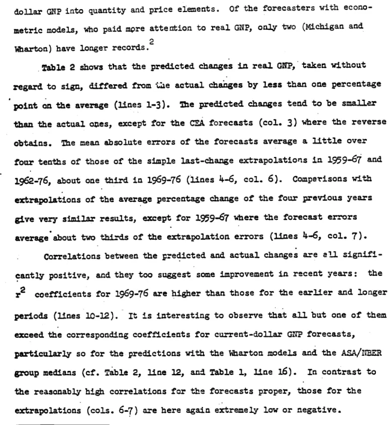
Table 2 shows that the predicted changes in real GITP, taken without

regard to sign, differed from the actual changes by less than one percentage

point on the

average (lines 1-3). The predicted changes tend. to be smller

than

the actual

ones,

except for the CEA forecasts (col. 3) where the reverse

obtains. The mean absolute errors of the forecasts average a little over

tour tenths of those of the simple last-change extrapolatiorts in 1959-67 and

1962-76, about one third. in 1969-76 (lines i+-6, col.

6).

Comparisons with

extrapolations

of the average percentage change

of

the four

previous years

give

very similar

results,

except for 1959-67 where the forecast errors

average about two thirds of the extrapolation errors (lines I_6,

ccl. 7).

Correlations between the predicted and actual changes are

eU

signifi-cant].y positive, and they too suggest some

improvement in recent years: the

r2

coefficients

for

1969-76 are higher than

those for the

earlier

and

longer

periods (lines 10-12). It is interesting to observe that all but one of

them

exceed the

corresponding

coefficients for current-dollal GNP

forecasts,

particularly

so

for the predictions with the arton models and the

ASA/1BER

group

medians

(ci. Table 2, line

12,

and. Table 1, line

16).

In

contrast

to the reasonably high

correlations

for the

forecasts

proper, those for the extrapolations (cola. 6-7)

are here

again extremely low or negative.

2Some

of

the econometric forecasts were released. at more than one date

near the end.

of

the year, and. in more than.

one

version depetid.ing on

the

data used or policy assumptions made. In all but a few doubtful instances where

somewhat arbitrary decisions had to be made, the forecasts chosen are those preferred. by the forecaster or, lacking stated preferences, those which embodied assumptions most common to the forecasts made at the time.

TABIZ 2

J)*ART MEASURES OF ERROR OR AXft1UAL PREDICTIONS

07PERCENTAGE (LANGES fl REAL GNP, 1959-76

lAce .

.

O• 0 55•3 Cove Selected Private Forecasts, Mean& (1.)

ASAJNBER Ecoctcrsic

trapolations

Actual

Survey, Reoort

Michigan arten

Median of the Mode Model List Average

Prelim-Forecast ?resideatb

ange

ange

inoy Revised

(2) (3) (Ii) (5) (6) (7) (6) (9)

1• 1959-67 (9)

.

'.1.

Mean Abaolate Percentage aage, Predicted and Actual

3.7 S

3(,0)C

2 1962-76(15) Lu 3.8

Li.

Lo

3 1969-76 (8) 3.3

Lo

3.5 3.2 3.6 3.3

.

-MeanAbsolute ror, in Percentage Peints

1959-67 (9) 1.3 1.0 2.7 1.7 5 1962-76(15) 1.1

1.

2.8 2.6 6 1969.-76 (8) 1.0 1.2 1.6 0.9 3.7 3.6 0.3 •

7

8 1959-67 (9) 1962-76(13) -0.9

Mean s•or, in Percentage Points

-0.5 -o.6 -1.1. -0.2 o.6 0.2 -0.3 0.1 -0.1. 9 1969-76 (8) • 0.7 0.8 0.8 0.5 -0.15 0.7 0.06 10 11. 12 1959-67 (9) 1962-76(15) 1969-76 (8)

.5

Squared Correlatioa (re) Between Predicted.531 306dand Actual

ange

.775 .617 .012

.936 .857 .709 .9k]. .001. •320d

Thr sources and explanations of the data used in columns 2-9, see footnotes it through k, respectively, in Table 1. CAverage of end-of-year annual forecasts of real. GD? inferred from the forecasts of current-dollar GD?, the

consumer price index (CPI) and the wholesale price Index (WPi) from the following sources: (1) harrIs Trust and Savings Back; (2) 1atioaal Securities and Research Corporation; (3) :1C3 (Conference Beard) Eonoeic Torum; (Ii) Robert W. Paterson, University of Missouri; (5) UClA Business Forecasting Project. Trese forecasts were obtained by dividing the forecasts of GD?, as reported in current dollars, by the composite price level

fore-casts, the latter are weighted su.-os of the reoorted forecasts of C?I and U?!, the weiitz being .67 and .353,

respectively (the first of these proportions represents the average ratio c'f sonsunption expenditures to GD? in

the period _L93-9). For further detail and analysis or the individual forecasts in this set, see Zarnowitz,

1968. See

also Table 1, f'n.b. —

-forecasts for 1962, 1963, 1965, end 1968 must be inferred from statements iAthe Report; they are con-firmed by the Council as approximately' correct, though ot in all caoes orecisely correct Moore, 1977). The other forecasts are all, based on figures given in the Reoort and so fully verified.

figure in psrentheaes is based on prelimina.ry CLIP figures deflated by weIghted averages of the corresoond-Lug data for CPI and UP! (with weights as given in fn. a above). This series of "actual" values is comparable to the forecasts used in column 1 onLy.

These

surnary

measures, then, present te annual forecasts of

real GNP

in a generally favorable light. However, the accuracy of these forecasts

varied greatly in

different

years, which at times impaired seriously their

usefulness, and this does not show up

in

the snmmry. As suggested by the

averages with regard to sign (lines 7-9), the usual tendency

of forecasts to

underestimate changes prevailed in

the

first half of the period 1959-76 but

cot in the second. half. Actually, the errors varied considerably in. each

sub-period, primarily reflecting cyclical change and. in

particular

the disturbing

effects of missed downturns. Real. GNP turned down in

l951.,

1958, 1970, and.

19Th1.,

but of the 10 predictions for these years which are available eight

specified continued rises and only two succeeded in signaling declines.

Main, and not surprisingly, nearly all of

the

significantly large

over-etimatioa errors refer to the years during which national output grew at

relatively low or decreasing rates, and, most of the larger u.nderestiination

errors refer to the years of high real growth rates.

It is of considerable interest to note that the tn'ning-point errors

are much larger than other errors (on the average about 2 1/2-3 times larger,

for all forecasts in this collection). Thus, even though relatively few,

these directional errors had, a strong adverse impact on the overall accuracy

of

the

real GNP forecasts, as indicated by the following tabulation.

Mean

Pbso1ute

Percert of Total

Number

Error, %

Points

Absolute Error

Underestimation errors ₃₃

1.12

Overestimation errors

21

_0.92 214.11.

little

because they are few arid. far between (cf. Samuelsori). Bat the argument

goes further to say that such few large errors are the necessary (and small)

price to pay for the avoidance of many large errors "between turning points"

by means of optimal estimation procedures such as least squares. However, it

is not clear that these procedures imply more than that the variance of

the

pred.icted.

changes must be less than that of the actual changes (and

progres-sively declining as the forecast span is lengthened.). The inevitability

(indeed;

even the existence) of a trade-off between errors at major turning points and other errors has never been demonstrated, and it would seern a e.u.nsel of despair for the forecasters to accept it. Prediction-of cyclical turns in such

series

as real GIP, though certainly difficult, is oat

nieces-•

sarily impossIble,

particularly on an annual basis (note the good record. in forecasting troughs). In sum, there are indeed. strong reasons for makers arid.

users

of economic forecasts to give a great deal of attention to

turning-point errors.

Actually, most of them realize this, as shown by the widespread practice of analyzing such errors (Hicinan, ed., 1972; studies in I.E.R.,

19714._75). However,

there is certainly much

need for improvement here, and room for some new initiatives (e.g., on. how to use current signals from leading indicators, see Vaccara and. Zarnowitz).

The worst single year for the predictions covered. in Table 2 was 19714.,

on

the e'e of which forecasters across the field missed the onset of a serious recession. This, plus the smaller turnin;-Doint errors for 1970, are

the

main reasons for the rise in the average errors of these forecasts in

1969-76

compared

with the earlier years. But the rise in. the absolute errors _{was not}

large, and there was no decline in accuracy as measured by the criteria of cumparisoris with extrapolations and correlations of predicted with actual changes

(Table 2, cols. 3 and ii.).

Limited evidence

_{from one longer series of}

suggests that real P

predicted

similar average errors in

the two 8-year periods 1953-60 and. 1969-76, with much smaller errors in the

relatively quiet

years 1961-68.

Although the

forecasts

of real

(NP are about as

good. relative to our

simple

extrapolative

bew4imk

models as are

the forecasts

of GNP in current

dollers,

they

are less accurate in terms

of

comparisons of the

errors

with

the

actual percentage changes to be predicted.

_{The point}

is that the

extra-• polations perform substantially better for

noniaal GNP than for real GNP.

This can be shown

by

dividing the error

of

extrapolation

into the

size of

the

actual

change, without regard

to

sign, which

_{gives the following overall}

ratios for the

Xl (last changc) and. (average change) models:

•

(P-—U, o.14; X2, 0.30

Real GNP-—Xl, 0.78; X2, o.68

These

results accord with

expectations, since the growth rates in constant—

dollar G1'P varied

considerably more

than

those in

current-dollar GNP.

The

ratios of forecast error to extrapolation error

average

about 0.l. when Xl is

the

standard, 0.5

to o.6

hea C2 is,

and. the results are

much the

sane

for either

variable.

Table 3 surveys the performance of forecasts of percentage changes in

the price level (I) that match the real G predictions covered in Table 2. On

the average, the

predicted inflation rates fall short of the actual ones by

fractions of one percentage point (flues 1-3). The 1959-67 forecast sets are less

accurate than

_{simple last-change extrapolations (line Li.), and the other} sets outperform the naive models by relatively small margins, much less than those observed for the series. The naive models work comparatively well here, with errors averaging about 3/10 of the actual changes in IPD.

PCV.CE AGES UI E IRICE L.EVFI, 1959-76 . Line Period

,,

Noor Tears Covered Selectet Private ThreCasts, Meana (1)

A$A/L Zcnonic

_trapolations Actu.ai.

survey, Roort Michigan ata.r-tna

Median

o the

Model Model Last Average

Forecast Presidetb

iange

aoge J

(2) . (6) (7)

Prelin-iaz

Revised

(8) Mean Absolute Percentage ange, Predicted end Actual

1. _{.195947 (9) 1.5 1.9}

l.9(1.le)° 2.0

2 _1962-76(15) . _{3.7 3.8} 3 _{1969-76 (8) 5.3 5.0 5.3} .

.2

5.9 6.2

Mean Absolute ror, in Percentage Points

1959-67 (9) 0.6 _{0.7 0.3 0.7}

5 1962-76(15) 1.0 1.0 _1.3

1.

0.i

6 1969-76 (8) 1.3

1.

1)1. 2.0 2.1.

0.

Mean ror, in Percentage Points

7 195947 (9) 0.2

0

-0.1. 0.0i _-0.3

8 _{1962-76(15) 0.5 -o.5 -0.2 -1.0}

9 1969-76 (8) -0.9 -0.6 -0.9

.0.6

-0.2 -1.2

.0.

10 1959-67 (9) .389

Sqnared correi.atioa (r2) Between predicted and Actual acge

1]. 1962-76(15) •

.768 .682 _{.536 .508}

12 _{1969-76 (8) .526 .581 .5ie}

.6o

_.166

.059

LTE: Forsources and explanations of thedata used_{in colunns 2-9, see footnotes d t.roug k, respective1', in Table 1.}

'Average of end-of-year annual forecasts of the conposite price level (a weighted su of forecasts of CPI and WPI)._{Se. Table 2, tfl. a, onthe weights used and sources.} bse. Table 2, rn. b.

figure in parentheses is based on weighted averages of data for CPI and UPI. This

series of actuals for the

cposite price level, is conparable to the forecasts used in coluna 1. onl,y (ct. Table 2, fo.

c).

change (cols. 6-7), which is the reverse of the situation for GNP in both

current and. constant dollars. The forecasts underestimated strongly (much

more than the last-change extrapolations) the average inflation since 1961

(lines 7-9). The predicted and. actual percentage changes in the price level

are all positively correlated, but the correlations for 1969-76 are generally

lower than their counterparts for (TP and, still more so, for real GNP (lines

10-12).

Forecasts of inflation often have much in common with projections

of the

last observed rate of inflation. To illustrate, correlations between the

errors of these forecasts and the errors of the correspond.ing extrapolations

produce the following

r2

coefficients:

Michigan, 1959-76: 0.51; CEA,

1962-76: 0.78; ASA/NBER, 1969-76: 0.95; Wharton, 1969-76: 0.80. For growth

rates in real G1'TP, the correlations between forecast errors arid, extrapolation

errors are also

positive but

throughout lower, in most cases much lower.

These

results are not surpristng and they

have a positive aspect inasmuch as

forecasts shou.ld be closer to extrapolations of a given

type in

those cases where such extrapolations are

more

effective (for an elaboration, see Mincer

and. Zarrio'witz). However, our

comparisons

are

constrained

to naive

models

which presumably do not represent

high standards

for

economic forecasting. In particular, price-level forecasts that are

highly correlated

with

last-change

extrapolations

must share the property'

of

the latter to lag

a

_year

behind the actual

rates of inflation. Indeed, the correlations between the

predicted

changes and

the

previous year' actual changes are

all

positive

and. high: the r2 coefftcients for the four

sets

of IPD

forecasts

listed

earlier in this paragraph

are 0.76,

_0.87,

0.81,

_{and 0.72, respectively.}

The annual percentage changes in real GNP

are inversely

related to those

two

variables do not show a strong

or stable association. The

relationships

between the predicted changes generally parallel the actual ones. This is

illustrated

by the r2 coefficients tabulated below (for symbols, see Table 1i).

1962-76

1969-76

Actual

Michigan CEA Actual Michigan

CEA

RCP-IPD

.567(-) .328(-) .528(-J

.61i6(_)

.l72(-)

.65l(-)

RCNP-CNP

.297

.210 .222 .614J .1.61i

.91

I-GNP

.020

.217

.o68

.o85(-)

.oo

.o22(-)

The

errors of the forecasts are similarly interrelated. Table Ii.

demon-trates a

pervasive pattern of

negative correlation between errors in

fore-casting

real growth and

inflation

_{(col. 1).}

The tendency

for these errors to

be

offsetting, which benefits the forecasts of P in current dollars, is

most strongly in evidence for the more recent years. When forecasters

over-estimated real

growth,-

or missed a downturn and projected continued growth

instead, they typically also underestimated inflation, as in 1969-71 and

l973—7.. Underprediction of real growth occurred in 1972 and 1975-76 in

combination with overp,rediction of' inflation.

These observations, which have some precedents (Zarnowitz, 1969; Moore,

1969,

1977), are

consistent with a view of the world in which

nominal GN'P

changes are predicted directly and relatively well, but their division

into

real and. price changes continues to pose great

problems. Many forecasters may

agree

with that view in general terms, and. some subscribe tà models consistent

with it (a specific excznple might be the St. Iuis model in which the dollar

change in total GNP expenditure is determined mainly by

the

dollar change in

a measure of money stock). However, most macroeconometric models, including

the two sets covered here, have separate aggregate real demand, output, and

TABLE .

CORRELATIONS BETWE ERRORS OF FORECASTS OF PERCENTAGE CHANGES

I NONA.L ONP, REAL GNP, AID lID, 1962-76

Squared. Correlation (r )

Between Forecast Errors

for

for

for

Line

Source of i1orecast

RP and. IPD RGNP and. ? lID .nd. (P

(1)

(2)

(3)

1962-76 (15 years)

1

Economic Report (CEA)

.297(-)

.359

2

Michigan model

•191.()

.129

.006

1969-76 (8 years)

3

Economic Report (cEA)

.677(-)

•o1i

.259

Michigan model

.68i.(-)

.209

.O]Ji

5

hartoa

model

.311.O(.)

.036

.li.66

6

ASA/NBER

survey, median

.52.(-)

.013

.351

NOTE: The smbo1s RONP, lID, and (TP denote real GNP, the ip1icit price

deflator, and. nomina.]. GNP, respectively. The correlations (r) are

positive, except there the sign (-) following the

r2 coeffiient

indicates that r is negative.

better in current than in constant dollars. In fact, so'e studies of the

recent

performance of quarterly

models

arrive

at the cpposite conclusion,

namely that

the results for real G are better than those for nominal GNP

because

of

deficient price

forecasts

(iggal, .ein, and

McCarthy; Eckatein,

Green, and. Sinai). The available evidence seans too lirnited and. too mixed.

to permit any conclusive generalizations on. this point. But it is interesting

to observe that the importance o± output errors vs. price errors ay vary

with changes in the relative roles of

real

vs. nominal factors and disturbances:

in

the

1970's the errors of the GNP forecasts were for the

most part

better

correlated. with the IPD

errors

than with the

RGNP errors, whereas in the 1960t

the contrary situation obtained (Table II.,

cols.

2-3).

IV. Quarterly Multiperiod Forecasts, 1970-75: An Overall Appraisal

Here we have space only for a

summary of

some early

results

from a study in progress. The forecasts and actual data are

used in

the same form as before, but they now refer to overlapping sequences of quarters, ot simply to a series of successive years. Our materials cover 22 quarters from 1970:3 through

1975 :, a period for

which

forecasts from several new sources are available. First

estimates for the

preceding

year, taken

from the

data prior to the 1976

benchmark

revision of the national income accounts, serve as

comparable

reali-zations. The full version of the study will include also comparisons with the

revised

data in an integrated treatment of forecast errors and measurement

errors. Adjustments of the

forecasts for base revisions, used in

some fore-cast evaluations, are regarded as questionable and. are avoided.

The mean absolute errors of GNP

forecasts

are close to one percentage point (like the annual forecasts, see Table 1) for two quarters ahead, and about

half

of

that or less for one quarter ahead. Over longer spans, the MAE

rise more or less steadily by

increments

varying

from

0.3 to 0.5 of one

per-centage point for each additional quarter; they approach

and exceed 2 percen-tage points for l1.-quarter and 5-quarter spans, and 3 percenpercen-tage points for 7-quarter and. 8-quarter spans, respectively (Table 5,

lines

1-3). Consistent with earlier findings and interpretations for various types of multiperiod

forecasts (see, e.g., Zarnowitz, 1967, pp. 60-72), the MAE increase less than in proportion to the extension of the span. The errors in forecasts of

percentage

changes expressed on a per-unit-of-time basis (roughly, errors

divided

by the length of the effective span) neither rise nor decline syste-matically as the forecast reaches further into the future. The same applies to the errors of the implicit predictions of changes during the successive

TABLE 5

StTh'fl1ARY ASUPES OF ERROR FOR QUARTERLY MtJI2IPERIOD

PRICTIONS OF PERCEITAGE CEANGE m

P,

1970-75

ne

Forecast

Seta

Span o± Forecast in Quartersb

One Two

Three

Four

Five

Six

Seven

(1)

(2)

(3)

(ii.)

(5)

(6)

(7)

Eit

(8)

Mean Absolute Error, in Percentage ints ()C

1 2 3 Chase DRI GE .14.2

1.03

1.32

i.68

2,22

2.73

3.19

.53

1.014. 1.11.3 1.911. 2.11.3 2.69 2.95 .11.2 .95 1.311. 1.71 2.19 2.59 2.88 3.11.9

2.80

3.25

Mean Error, in Percentage ints Ii. 5

6

Chase DRI .01 .014. .02 .08 -.111. -.66 -1.11.8

-.01

.11 .05 .11 .01 -.1i.2 -1.12 -.JA -.15 -.30 -.15 -.15 -•144. _-.95 -2.311. -1.69 -1.68

Squared Correlation (r )

Between

Predicted and. Actual

Change

7

8

9

Chase DRI GE .752 .11.51 .107 .058 .127

.l31.

.179

.632

.11.69

.069

.000*

.008

.102 .211.9 .753

.577

.2811. .159 .132 .180 .227

.293

.6oo

.225

Theil's Inequality

Coefficient

(U)e

10 II

12

Chase DRI GE .211.1 .287 .291 .268 .236 .218 .198 .2811. _{.292 .299} .295

.272

.218 .182 .215 .260 .260 .211.3 .233 .204 .181 .189 .ili.8 .172

aChase. Chase Econometric Associates, Inc.; DRI:

Data Resources, Inc.; GE:

MAPCAST

group

at the General Electric Company. The forecast data are

those ased

and

described in

S.

K. McNees, 1975, 1976.

Chase

and DRI are

"early-quarter

forecasters,"

while GE

is

a "late-quarter forecaster" (for the release dates, see McNees, i976,

p. 11.1).

bNer

of

forecasts covered (a) for spans 1 to 7, respectively:

22, 21, 20, 19, 18, 17, and

16

(for each of the sets). For span 8,

the

number is 15 (Chase), 111.

(DRI), and 12 (GE).

CDefining the predicted change and

the

actual change (for the given set,

variable,

1

period., and span) as _{and. At,}

respectively, MAE =

E

e ,

where

et =

- At.

d.

single quarters covered; it is the cumulation of these intraforecast (umarginalfl)

change errors that technically accounts for the tendency of errors in the total predicted changes to grow with the span.3

Vhere

both forecasts and realizations refer to increases (as

they do

most of the

time by far

in

the case of ip), rrors of positive sign denote

overestimation

of actual change. The mean errors in Table 5, lines 14._6,

are

predominantly

small and. positive, except for the longer spans where some of

them are

large

and. negative. As will be shown below,

these averages conceal large errors of opposite sign in the forecasts for some

of the different economic phases of the period 1970-75.

2

The

r coefficients for the correlations between the predicted and.

actual changes In P exceed o.6 or 0.7 for one quarter ahead (like the annual

forecasts)

and. exceed. Q•1.

or 0.5 for two quarters ahead. They

are

much smaller for

the

_longer

spans, mostly in the 0.1-0.25 range,

in

a few cases near

zero

(lines 7-9).

Theil?

s inequality coefficients generally fall between 0.2 and

0.3

(lines 10—12). This indicates

that these forecasts are all much better

than

a naive model extrapolating the last recorded percentage change

(for

which

U =

1).

That model, it should be noted, is but a minimal standard

for

economic forecasts. Interestingly, the

U coefficients do not increase

with the forecast span;

in

fact, they decline slitly below .2 for the

longest

spans.

The

next

two

tables

have the sane format as Table 5,

which

facilitates

presentation

and comparisons of these measu.res. Real GNP forecasts have MAE (in percentage points) rising from o.-o.6 for one quarter ahead

to

-6

for

3Note that fewer observations are available for the longer spans (Table 5,

b). This reduces the comparability of the measures reported for the

differ-ent spans, but does not

eliminate it.

6

SUMMARY ASUPES OF ERROR FOR QUARTERI?L MTJLTIPERIOD PREDICTIONS

OF PERCE1TAGE CHANGE m REAL GNP, 1970-75

.

Line

Forecast

Seta

Span of Forecast in Qjlartersb

One

Two

Three

Four

Five

Six

Seven

Eight

(1)

(2)

(3)

(ii.)

(5)

(6) (7) (8)

Mean Absolute Error, in Percentage ixits ()C

1

Chase

.51

1.11

1.81

2.11.6

3.29

11..19 )4..95

5.31

2

DRI

.61

1.37

2.08

2.75

3.52

4.15

4..78

3 GE

.50

1.20

1.75

2.15

2.80

3.80

14..76

5.15

Mean Error, in Percentage PDints ()d

14.

Chase

.17

.51

.92

1.11.6

1.98

2.38

2.63

2.82

5 DRI

.26

.77

1.20

1.82

2.59

3.16

3.66

_14..72

6 GE

.00

.22

.36

.9

1.53

2.09

2.11.6

Squared Correlation (r2) Between Predicted and Actual

2.58

Change

7

Chase

.839 .81'7 .727

.703

.733

.710 .6o14.

.596

8 DRI .793 .711.5 .598 .814. .785 .827 .711.1

.638

9 GE .808 .711.1

.677

.607

.772

.7614.

.661

.662

e

Theil's

Inequality Coefficient (13)

10

Chase

.11.33

.502

.607

.673

.711

.74l

.758

.711.1

II

DRI •5O1

.622

.721

.769

.781 .7711.

.771i

.836

12

GE .11.27 .1198 .511.8

.606

.627

.676

.71ji

.6911

eight

quarters ahead, that is, somewhat more than in proportion to the measured

span

(Table 6,

lines

1-3). The errors for the two

shortest

spans are

not

much

larger than those for GP in current dollars, but the errors for the longest

spans

are 50

to

100 percent larger. The u.nusually rapid build-up of the MAE

can be traced in large part to turning point errors. In quarterly multiperiod.

forecasting, turning points are more frequent and more difficult to predict

than

in

annual forecasting, but the errors associated with them matter much

more yet: here, missing a turn often means that a whole chain of predictions

for the

subsequent observations is badly off.

The mean

errors of these forecasts are

all

positive, which is largely

due to the effects of missing or underestimating the declines in real GNP

during

the recession (Table 6,

lines

1i.6).

The

also cumulate continuously

and. rapidly

here, quite nriltke those for the

nominal GNP

forecasts. On the other hand, the r2

coefficients

are

rather surprisingly high in Table

_6,

lines

7-9, much above the corresponding figures for (2P

in

Table 5,

particularly

for spans of 3-8

quarters.

Relative to the size of

the

_{actual changes, however,}

the real (P

errors

are

much

_larger

than

the current—dollar GNP errors:

the inequality coefficients rise from •14—.5

to

.7—.8

(Table

6,

lines

10-12).

The

MAE of

forecasts of inflation in terms of the P

implicit price

deflator

are like those of the (p forecasts for the shortest spans--O.5 or less one quarter ahead, approximately 1

percentage

point two

quarters

ahead--but

they cumulate rapidly, especially for the longest spans (Table 7, lines

1-3). The figures for the eight-quarter-ahead predictions are

here

more than

12 times as large as those for the one-quarter-ahead predictions. This

exceptionally

strong build-up of errors reflects a progression of under-estimates of the inflation rates, rising more than in

proportion

to

the

_span

TABLE 7

SIThARY ASURES OF ERROR FOR QUARTERLY MtJLTIPERIOD PREDICTIONS

OF PERCENTAGE CEANGE fl E PRICE LEVEL, 1970-75

ne

Forecast

Seta

Span of Forecast, in Quartersb

One

Two Three

Four

Five

Six

Seven

(1)

(2)

(3)

(14.) (5) (6)

(7)

Eight

(8)

Mean Absolute Error, in Perceiltage Points (MA.E)C

1

2

3 Chase .39 1.02 1.61;. _{2.29 2.98 3.87} 4.88 DRI .514. 1.11 1.69 2.37 3.05 4.01;. 5.17 GE .39

.90

1.11.9 1.96 2.37 3.06 4.o8 5.69 6.78 4.79

Mean Error, in Percentage Points ()d

1;.

5

6

Chase DRI GE -.15 -.11.9 -.96 -1.50 -2.33 -3.31 -.27 -.70 -1.22 -1.85 -2.82 -3.88

-5.12

-.12 -.36 -.70 -1.20 -1.85 -2.78 -3.76

-.48

-6.78 -4.57 Squared Correlation (r2) Between Predicted

and. Actual

change

7

8

9

Chase DRI GE .6oo .11.40 _{.3911. .287} .211.6 _{.233 .320} .14.78 .426 .412 .346

.4oi

.398 .384 .657 .633 .5o8 .11.40 _{.11.38 .457 .524} .381 .371 .676

Theil's Inequality Coefficient (U)e 10 11 12 Chase DRI GE .311 .358 .377 .410 .438 .462 .480 .375

.38

.397 .422 .444 .475

.508

.284

.286

.326

..3514.

.369

.395

.4i6

.496 .540 .410

The

r2

coefficients for the IPD inflation forecasts are

generally

higher than those

for the forecasts

of percentage change in

nominal GITP

(except

for a few short predictions) but throughout lower

than the

correspond-ing statistics

for the real growth forecasts. They range from .23 to .66

and

tend to decrease as the spans lengthen (Table 7,

lines

7-9).

The

U

coeffi-cients (lines 10—12) are close to .2 for the shorter spans and close to .5

for

the longest; they are thus higher than their counterparts for the current—dollar GNP forecasts but lower than those for the real GNP forecasts.

The quantity

and price ingredients of the TP

forecasts show a pattern of offsetting errors in the

quarterly

as

well

as annual data. The irtean errors of real growth predictions are aLl, positive, those of inflation predictions

all negative, and. these statistics, matched by source and span, have similar absolute values for most of the shorter forecasts As a result, the ?€ of the current-doll:ar tP forecasts for spans 1_li. are as a rule positive but very

small

for chase and DRI, negative but small

_{for GE. The negative of the} inflation

forecasts outweigh

the positive of the real growth forecasts in spans

5-8, so that the

of the percentage change

forecasts

for P

_are

pre-dnmiriantly

negative and substantial (of. lines k-6

in

_{Tables ,}

6, and

_7).

The

surveyed accuracy measures

do not show any

of the forecasters to be

consistently superior to the others. They do

favor

GE over Chase and.

DRI in

most instances, but by modest margins

and in a way that

can be explained

_{by an} advantage in timing:

the

GE forecasts

are issued late in

each quarter, the others early.

The

results reported in this study should and will be carefully conipared with those of other evaluations of the same forecasts, but the task is still to be completed.

The

error

measures used here differ in

_{several respects} from those used by others,

and additional

_{computations are required to allow} for these differences.

V. Quarterly Multiperiod Forecasts: An Analysis by Su.bperiods

The period l97O:3-l975:4, although short, was unusually

varied

and.

marked by major disturbances arid drastic changes in the economy's course. It is

useful to divide it into the following parts, as suggested by the contemporary

business-cycle and inflationary developments.

I. 1970:3-1973:1. End

of

the

mild.

1970

recession

followed by an

expansion that accelerated in 1972, with relatively

stable inflation.

II.

1973:l_1973:!.. Slower real growth and a sharp inflation speedu.p

(materials

shortages, run-ups in commodity prices, oil embargo).

III. 1973:1._1975:1. Recession, severe in its last two quarters, accoin-panied first by

a further

rise

and then by a

dxwri-turn in the rate of inflation.

IV. 19'7:1_197:11. Sharp

upturn arid

the initial recovery phase, with

a further decline in inflation.

One question is whether forecasts that originated in these four

sub-periods show significantly different characteristics and performance. The

other is whether forecasts for these subperiods (i.e., those that aimed at

the

corresponding groups of

target quarters) are

so

differentiated. It turns

out

that the answers to both questions are definitely yes.

To illustrate the first point, the expansion phase I produced forecasts that underestimated growth in dollar GNP mainly because they underestimated inflation. The percentage changes in real GNP were partly underpredicted, partly (in some longer forecasts) overpredicted, but whether negative or positive the of these forecasts were small. In general, the record of the

forecasts

that were made

during the

_period

I was good in tezs of both the ME

and

the MAE figures, even for the long spans. In contrast, the slowdown phase

II produced real growth

predictions with very large positive ME and inflation

forecasts with

very large negative

ME (widerestimation errors).

These errors balanced each other so that

the

ME for the nominal

GMP predictions

were

moderate (and mostly

_negative,

except for the

_{longest forecasts).}

The

recession phase I gave rise to even larger positive mean errors in the real growth

forecasts as the declines were repeatedly missed anii,

when finally recognized,

underestimated. These errors were larger absolutely than

the

negative

errors on

the price side, which reflected a continuing underestimation

of

inflation, so that the predictions of' the growth rates

in nominal GNP

had

consistently

positive ME in

the subperiod

III.

The above sIimrny is based on charts (not reproduced here) which show

the average errors (MAE and

ME) by

span

and

by subperiod. in which the

fore-casts originated.

These charts look very similar for such different models

as Chase and DRI: they show in each case the same strild.ng differences

between the forecasts made in

subperiods I,

II, and III. The suggested

infer-ence is that concurrent predictions from different sources and models have common patterns such that their errors depend strongly and similarly on the characteristics of the time of their origin.

In a second exercise, the forecasts were assigned to the four stibperiods according to their target quarters,

not their base

quarters, as illustrated

In

Charts 1-3. Here the samples are

partitioned differently, hence the resulting patterns

diverge from

those obtained on the

first plan, but the

LI. .

No averages for phase IV are used on this basis, since they contain too few observations in the truncated. sample.

conclusion

is analogous: the type and size of forecast errors depend criti-cally on the economic properties of the target periods vis--vis

those

of the periods of origin. Forecasters perform best when the two

periods

are alike,

belonging to the same already recognized phase, e.g., a continuing expansion as in 1971-72

(most of

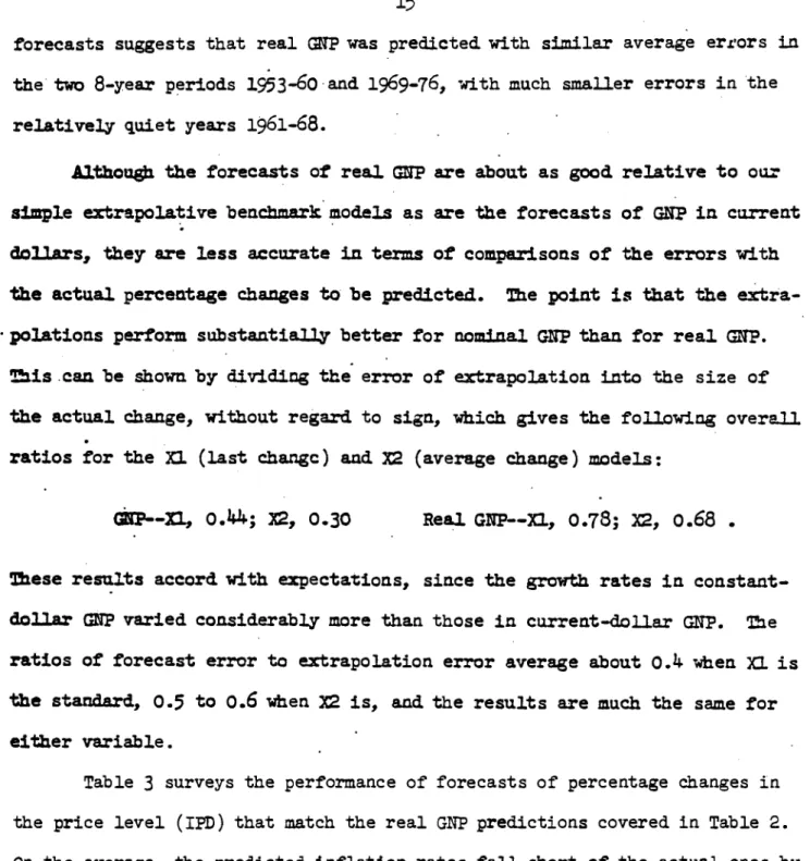
subperiod. I). They perform worst when the target falls into a new phase, particularly when the latter departs sharply from the currently established pattern (forecasts made in. subperiods II and. III, and those for subperiods III and. IV provide many examples, particularly in the long-span categories). Such period characteristics are much more important determinants of forecast errors than are any differences among the forecasters.

Chart 1 shows that both Chase and DRI persistently underestimated the

percentage changes in GI'TP for su.bperiods I and., much more strongly, II. Both

forecasters overestimated the changes in their short forecasts for subperiod III and. underestimated them in their long forecasts for the same phase.

Over-est.mates prevailed. in all forecasts for the last phase covered., IV, and. here

the average errors behave in an unusual fashion, first increasing and then decreasing with the lengthening span.. This is due to offsets between. the real growth forecasts with positive ME and the inflation. forecasts with negative ME (see Charts 2 and 3).

Chart 2, which covers the real growth forecasts, shows u.nderestimates

dominating the errors for I and. II, much larger MAE aud. positive lylE for III

and. IV. The huge average errors for the two latter phases derive mainly

from the forecasters' failure to predict the declines in real GNPI5 The long-span errors for the 1975 recovery (IV) are strikingly large here.

5The change _errors,

-At

(see Table 5

for

the symbols), are positive

where P >

0 and.

_{At < 0,} and. also where

< 0 and At < 0 but

At. These cases dominate in Chart 2 the results for both the recession phase III and. the recovery phase IV. Although real GNP reached a trough in 1975:1 and increased thereafter, the actual changes over longer spans ending in 1975 are negative; that is, real GNP was lower during period IV than in.

r4 0

.Ia

4

:

0

OP4

r4

vw) .zo.z.za iw 11 H C., a) a Ca S.' 4.' a -4 a 4, 04

:

'

S.' .43 -4H

I

4.' • 0 (Y(.r(\ç\

I

liii CL a (j) 4, . M 0Lr4 ..' r4r4H1 o

-

1-4 -4HHC jTrr i.

=

C-

H;ttt

:':

rr

1r

p.

/

.1.

r

4 -II

T'

:

-

1E'

1

1

•1 — •- -. -1.-I. 4-4

•

u; '(ni) .zo.z.z iN ,--;

i•

--

-H- ---+--

-,-

.,S

.-14I .4. — — —'— '±... •c-=

•:l:

'.3

I..

:

I

_____

I

i-i——r-r ________ _________

-

Ii\

cy (\O r C4

T

4h\

I

cI 0 — S.— ..+, -* Qi 0 0 iCaC424 a) •C.) C) C)

.

Cd Cd a

0

E r1000 C44C4..4 00 a H a)a) hull

Il

3

II

---im _:C.

Ij1ktj%J. QUARTERLY MULTIPERIOD FORECASTS OF PERCENTAGE CHANGES

IN

REAL GNP, AVERAGE ERRORS BY SUBPERIOD AND SPAN, TWO MODELS,

1970-75

11n9lffftrIifftrI

nn

5-I 5-I _{N H} 0 1-

IT

Legend:

See

chart