University of Nebraska - Lincoln University of Nebraska - Lincoln
DigitalCommons@University of Nebraska - Lincoln
DigitalCommons@University of Nebraska - Lincoln
Faculty Publications from the Department ofElectrical and Computer Engineering Electrical & Computer Engineering, Department of 3-2011
Support Vector Machine-Based Short-Term Wind Power
Support Vector Machine-Based Short-Term Wind Power
Forecasting
Forecasting
Jianwu ZengUniversity of Nebraska-Lincoln Wei Qiao
University of Nebraska–Lincoln, [email protected]
Follow this and additional works at: https://digitalcommons.unl.edu/electricalengineeringfacpub Part of the Electrical and Computer Engineering Commons
Zeng, Jianwu and Qiao, Wei, "Support Vector Machine-Based Short-Term Wind Power Forecasting" (2011). Faculty Publications from the Department of Electrical and Computer Engineering. 158.
https://digitalcommons.unl.edu/electricalengineeringfacpub/158
This Article is brought to you for free and open access by the Electrical & Computer Engineering, Department of at DigitalCommons@University of Nebraska - Lincoln. It has been accepted for inclusion in Faculty Publications from the Department of Electrical and Computer Engineering by an authorized administrator of
I. INTRODUCTION
Wind power forecasting (WPF) is a technique which provides the information of how much wind power can be expected at a given point of time[1]. Due to the increasing penetration of wind power into the electric power grid, WPF, particularly the short-term WPF, is becoming an important issue for grid opera-tion. A good short-term forecasting will ensure grid stability and a favorable trading performance on the electricity markets [2]-[3]. For example, Wang et al. [4] investigated the impact of WPF errors on power system operation with stochastic and determin-istic methods.
The existing WPF models can be classified into two catego -ries, i.e., physical model or statistical model. The physical model
is to refine the Numerical Weather Prediction (NWP) by using
physical considerations about the terrain such as the roughness,
orography and obstacles; while the statistical model aims at find -ing the relationship between the forecast-ing value and the mea-sured historical as well as current values. The physical model has advantages in long-term forecasting while the statistical model does well in short-term forecasting [5]. This paper focuses on the statistical model-based WPF.
The persistence model and the autoregressive moving aver-age (ARMA) model are two traditional linear models that are used in WPF. The persistence model is a classical benchmark model in which the forecast for all times ahead is set to the cur-rent value. The ARMA model works well when the distribution of wind speed is Gaussian. Torres et al. [6] evaluated the ap-plicability of the ARMA models to the prediction of the time-series of hourly average wind speed with certain transforma-tion and normalizatransforma-tion. Compared to the persistence model, it
turned out that the ARMA models can significantly improve the
accuracy of the prediction.
Nonlinear artificial intelligent methods, such as artificial
neural networks (ANNs), fuzzy neural networks, and sup-port vector machines (SVMs), have also been used for WPF. These models outperform the linear methods, e.g., the persis-tence model [7]. Kariniotakis used recurrent high-order neural networks for WPF [8]. Sideratos combined the self-organized map, radial basis function (RBF) neural networks, and fuzzy logic for WPF [9], in which future wind speed is provided by the NWP. Similarly, Pinson used adaptive fuzzy neural net-works combined with the NWP for short-term WPF [10]. Mo-handes compared the performance of a multi-layer perception (MLP) ANN-based model to the autoregressive model [11]. The performance of using a SVM and a MLP with different hidden units were also compared [12]. It was shown that the
MLP significantly outperforms the autoregressive model for
wind speed prediction; while the SVM compare favorably with the MLP model. However, other work indicates that SVM out-performs ANNs in WPF [13]. Furthermore, the SVM-based models were found to take less computational times compared to the ANN-based models [14].
This paper proposes a SVM-based model for short-term WPF. Simulation studies are carried out for the proposed model, the persistence model, and a RBF neural network-based model by using real wind speed and wind power data obtained from the National Renewable Energy Laboratory (NREL). Re-sults show that the proposed model outperforms the persis-tence model and the RBF neural network-based model. The paper is organized as follows. RBF neural networks and SVM are introduced in Section II. Section III describes data prepro-cessing for WPF. Simulation results of the proposed model and RBF neural network-based model using NREL data are provided and discussed in Section IV. The paper ends up with conclusions in Section V.
This material is based upon work supported by the National Science Foundation under CAREER Award ECCS-0954938 and the Federal Highway
Administration under Agreement No. DTFH61-10-H-00003. Any opinions, findings, and conclusions or recommendations expressed in this publi
-cation are those of the authors and do not necessarily reflect the view of the Federal Highway Administration.
Support Vector Machine-Based Short-Term Wind Power Forecasting
Jianwu Zeng (student member, IEEE) and Wei Qiao (member, IEEE)
Department of Electrical Engineering, University of Nebraska-Lincoln, Lincoln, Nebraska, U.S.A. 68588-0511 (E-mail: [email protected])
Abstract
This paper proposes a support vector machine (SVM)-based statistical model for wind power forecasting (WPF). Instead of
predict-ing wind power directly, the proposed model first predicts the wind speed, which is then used to predict the wind power by uspredict-ing the
power-wind speed characteristics of the wind turbine generators. Simulation studies are carried out to validate the proposed model for very short-term and short-term WPF by using the data obtained from the National Renewable Energy Laboratory (NREL). Re-sults show that the proposed model is accurate for very short-term and short-term WPF and outperforms the persistence model as well as the radial basis function neural network-based model.
Index terms: Artificial neural network (ANN), Radial basis function (RBF), Regression, Statistical model, Support vector machine
(SVM), Wind power forecasting (WPF)
2 J. Zeng & W. QiaoinProceedingsof the 2011 ieee Pes Power system conferenceand exPosition
II. RBF NEURAL NETWORKS AND SUPPORT VECTOR MACHINE
A. RBF Neural Networks
The RBF neural networks are a class of feed-forward ANNs constructed based on the function approximation theory. Figure 1 shows the structure of RBF neural networks, which contains an input layer, a hidden layer, and an output layer.
Generally, the input-output relationship of a RBF neural net-work can be described as:
(1) where x is the input; y is the output; m is the number of RBF units in the hidden layer; wi and w0 are the weight and bias be-tween the ith RBF unit and the output, respectively; φ
i(·), ci and
ßi are the activation function, center, and width of the ith RBF unit, respectively. The Gaussian function is the most commonly used RBF function.
(2)
where □ ·□ represents the Euclidean distance. The Gaussian
function makes the value equidistant from the center in all direc-tions have the same values.
Constructing a RBF neural network involves determining the RBF centers, width, and the output weights and bias. Two meth-ods are commonly used to determine the centers of RBF net-works. One is to select representative input samples as the RBF centers; the other is to determine the centers with a self-organi-zation method, such as the K-means clustering algorithm [15]. In this paper, the K-means clustering method is used to locate the centers.
Once the RBF centers are located, the width can be simply determined by [15]:
ßi =k ·dmax (3) where dmax is the maximum Euclidean distance of the centers and k is a nonnegative scalar.
After the centers and width are fixed, the weights can be deter -mined by a least-square method to minimize the error of the out-put. In this paper, the Netlab toolbox [15] is used, in which the singular value decomposition (SVD)-based numerical least-square method is applied to determine the output weights and bias.
B. Support Vector Machine
The SVM has been successfully applied to the problems of
pattern classification, particularly the classification of two differ -ent categories of patterns. The fundam-ental principle of
classi-fication using the SVM is to separate the two categories of pat -terns as far as possible. The basic idea of the SVM is to map data x into a higher-dimensional feature space via a nonlinear
mapping. Then the linear classification (regression) in the high-dimensional space is equivalent to the nonlinear classification
(regression) in the low-dimensional space [16].
y = w · Φ(x) + b (Φ : Rn → RN) (4) where y ∈RN is the output; x∈Rn is the input regression
vec-tor and x = [yt-1,yt-2, …, yt-d ]; b is a bias term; w∈ RN is the coefficient vector; and Φ: Rn → RN is a nonlinear feature map,
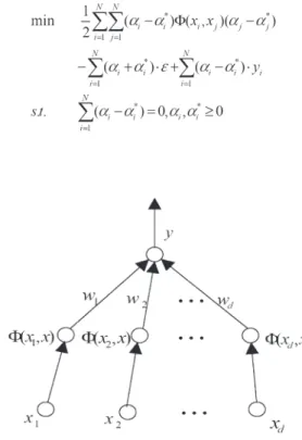
which transforms the original input x to a high-dimensional vec-tor Φ(x) ∈RN; the vector Φ(x) can be infinite dimension. Figure
2 shows the structure of the SVM, where the input x is mapped via function Φ(·); the output y is a linear combination of Φ(x).
A specific SVM called ε-SVM is used in this paper due to its scarcity representation capability. The samples locating in the ε tube are not taken as support vectors without losing the gener-alization ability. The objective function of the ε -SVM is based on a ε -insensitive loss function. The formula for the ε-SVM is given as follows:
(5) Such a quadratic programming problem is usually solved by solving its dual problem as follows.
(6)
After solving for the coefficients (αi – αi*) the final expression
for the estimation of y is given by:
(7) where K(xi, xj) = Φ(xi)Φ(xj). Based on the Karush-Kuhn-Tucker (KKT) conditions [16] of the quadratic programming, only a
certain number of the coefficients (αi – αi*) will assume
non-zero values. The data points associated with the nonnon-zero coeffi -cients having approximation errors equal to or larger than ε are referred to as support vectors. The samples in the ε-insensitive area are not support vectors and have no contribution to the es-timation. Generally, the larger ε, the fewer the number of sup-port vectors and the sparser the representation of the solutions. For given n samples, the ε -SVM solves a 2n×2n kernel matrix. The RBF [17] is used as the SVM kernel in this paper.
(8)
III. DATA PREPROCESSING
A. Data Description
The data used in this paper is the Western Dataset [18] cre-ated by 3TIER with the oversight and assistance from the NREL. NWP models were used to essentially recreate the his-torical weather for the western U.S. for the years of 2004, 2005, and 2006. The modeled data was temporally sampled every 10 minutes and spatially sampled every 2 kilometers. 3TIER mod-eled the power output of ten wind turbine generators (WTGs) at 100 meters above the ground level on each grid point using a technique called the Statistical Correction to Output from a Record Extension (SCORE) [19], which replicates the stochas-tic nature of the wind plant output. The dataset contains the in-formation of wind speed, the corresponding power output and SCORE-lite power, etc.
Sixty eight WTGs from a wind farm 10 miles west of Den-ver, Colorado are selected to validate the proposed WPF algo-rithm. The data contains the average wind speed and power of the 68 wind turbines at same times.
B. Resolution
The resolution of the original dataset is 10 minutes. Each data represents the average wind speed and power within one hour. For very short-term forecasting, the sample time is set as ten minutes for the implementation of the proposed WPF algo-rithm. For the short-term (more than 6 hours) forecasting, the sample time is set as two hours.
The transformation among different resolutions is based on the assumption that the data values between two adjacent sam-ples are linearly changed, that is:
(9) where dti is the time interval between xi and xi+1. Then for a given resolution TS, the average value of the data within TS can be calculated as:
(10) The average value is then used as the value of the data sam-ple by the proposed WPF algorithm. In this paper, TS = 60 minutes is used in the very short-term forecasting (less than 6 hours) and TS = 2 hours is used for short-term forecasting (from 6 hours to several days) [2].
C. Normalization
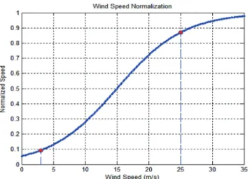
To avoid tuning the SVM parameters while the input data is changed, especially when the input has more than one variable with different ranges, the data x is normalized to the range of [0, 1] by using the sigmoid function.
(11) where µi and si are the mean value and standard deviation of the ith input data, respectively. There are two reasons of using the sigmoid function for data normalization. First, the sigmoid function can strictly map the original input, i.e., the real wind
Figure 3. Wind speed normalization.
4 J. Zeng & W. QiaoinProceedingsof the 2011 ieee Pes Power system conferenceand exPosition
speeds, to the range of [0, 1], as shown in Figure 3, the origi-nal cut-in and cut-out speeds are 3.5 m/s and 25 m/s, tively; the resulting normalized values are 0.1 and 0.87, respec-tively, which takes approximate 80% of the whole range of [0, 1]. Second, the mean value µi and the standard deviation si make the data translation, rotation, and scale invariant.
D. Feature Representation
Feature representation, which aims to extract certain charac-teristics from the original data, plays a key role in determining the performance of the WPF. Improper features obtained from bad feature extraction will lead to poor regression in the SVM. In this paper, wind speed is selected as an intermediate variable, which is predicted by the proposed SVM algorithm and RBF neural networks. The predicted wind speed is then used to cal-culate the wind power according to the power-wind speed char-acteristics of the WTGs. The reason of using wind speed as an intermediate variable for WPF is that wind speed is a continuous variable while wind power discontinues at certain wind speeds
(e.g., the cut-in, rated, and cut-off wind speeds). It is more diffi -cult to predict wind power than wind speed.
The embedding dimension of the SVM [16], i.e., the num-ber of previous data samples used as the input of the SVM, is
determined by the autocorrelation coefficients of the data sam -ples as follows.
(12) where µ and s are the mean and standard deviation of the first
330 days’ wind speeds in the dataset, respectively. Figure 4
illus-trates the autocorrelation coefficients of the wind speed sam -ples used in this paper, which shows that adjacent sam-ples are highly correlated. Given a threshold rT of the autocorrelation
coefficients, the embedding dimension can be determined. For
example, if rT = 0.8, then the former eight samples are used as the input of the SVM.
E. Fixed-Step Prediction Scheme
Given a prediction horizon of h steps, the fixed-step fore -casting means only the value of the next hth sample is predicted by using the historical data.
ŷ(t + h) = f (yt, yt-1,…,yt-d) (13) where f is the nonlinear function generated by the SVM. Fig-ure 5 shows such a prediction scheme, in which yt+h is predicted with the data before yt (the red blocks), yt+h-1 is predicted with the data before yt-1 (the green blocks).
Figure 5. The fixed-step prediction scheme.
F. Evaluation
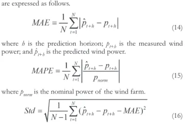
The mean absolute error (MAE), mean absolute percentage error (MAPE), and standard deviation (Std) of the absolute er-ror are used to evaluate the WPF performance [13]. Smaller val-ues of the MAE, MAPE, and Std imply a superior WPF
perfor-mance of the model. The definitions of MAE, MAPE, and Std
are expressed as follows.
(14) where h is the prediction horizon; pt+h is the measured wind power; and pˆt+h is the predicted wind power.
(15) where pnorm is the nominal power of the wind farm.
(16) The persistence model is used as the reference model to compare the performance of the SVM model and the RBF
model. A parameter called skill is defined as follows:
(17) where ep and e are the MAE of the WPF using the persistence model and the SVM (or RBF) model, respectively. A larger skill value indicates a better prediction performance of the model.
G. Parameter Selection
Three parameters, i.e., γ and σ2 of the SVM and the embed-ding dimension d, need to be determined. The value of the em-bedding dimension can be “read” directly from Figure 4. In this paper, the threshold rT is chosen as 0.8. Consequently, the value of d is chosen as 8 from the results shown in Figure 4. That means that the previous 8 wind speed samples are used as the input of the SVM to predict the wind speed at next several time steps. The values of γ and σ2 (γ = 50 and σ2 = 0.3) are obtained from an exhaustive search.
IV. SIMULATION RESULTS
Simulations are carried out to validate the proposed SVM-based algorithm for very short-term and short-term WPF. The re-sult is compared to that of the persistence model and RBF neu-ral networks-based model. The dataset is divided into two groups, i.e., one group of training data and the other group of testing data. The data of 7 days is selected as testing data, in which the measured average wind speed is 9.99 m/s. It should be noticed that the testing data is selected from those segment with more
significant variations. The training data contains the data of the
n days before the first testing data sample. Simulations are per -formed to numerically determine the size of the training data, i.e., the best value of n, for WPF using the proposed method.
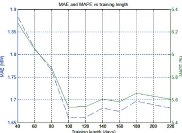
Figure 6 shows the MAE and MAPE as functions of the length of the training data (called the training length) for a pre-diction horizon of 3 hours. As shown in Figure 6, it is not true that the longer the better for the training data. The MAE and MAPE decrease drastically with the increase of the training length up to 100 days. However, after 100 days the MAE and MAPE increase with the training length. Therefore, 100 days is selected as the best training length, i.e., the value of n, in the fol-lowing simulations.
A. Very short-term forecasting
In the very short-term forecasting, the resolution (the time
interval between two samples) is fixed at one hour. The fixed
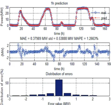
step scheme is applied in the forecasting. All of the predicted values are true out-of-sample forecasts, in which only the data samples prior to the prediction horizon are used. That is the models are estimated over history values. The predicted data is then compared to the actual measured value. The procedure is repeated for the next time step until it runs over the entire test-ing dataset. Figures 7-9 show the results of 1h-3h ahead predic-tions, respectively.
As shown in Figures 7-9, the predicted values follow closely the measured values. A large error occurs when the wind speed changes drastically. However, approximately 50% of the er-rors are less than 3.3%. The prediction results of the RBF model are shown in Figures 14-16 of the appendix for com-parison with the SVM model. Compared to Figures 7-9, the large MAE and MAPE values in Figures 14-16 indicate that the RBF model is inferior to the proposed SVM model. Fig-ure 10 shows the skills of the proposed SVM model and the RBF model as functions of the prediction horizon, where the persistence model is used as the reference model. The skills of both models are more than 62% for one hour WPF and 19% for six hour WPF. This indicates that both models signif-icantly outperform the persistence model. Figure 10 also indi-cates that SVM model has a better performance than the RBF model. This conclusion is the same as that in [13]. However, the skills decrease with the increase of the prediction horizon. The reason is probably the accuracy is deteriorated in both the proposed model and the reference model. The increased error of the persistence model worsens the skill when the prediction horizon becomes longer. For example, the skill reaches zero when the prediction horizon is so long that both models be-come ineffective. Moreover, from the perspective of statistics, the larger the prediction horizon, the more uncorrelated data used which leads to a larger error.
The parameters of the SVM model are fixed during the
testing stage. One of the concerns is the model effectiveness,
namely, how many days can be predicted accurately with the
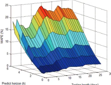
trained fixed model. Figure 11 shows the 3-D view of MAPE as
a function of the testing days and prediction horizon. As shown in Figure 11, the MAPE increases with the predict horizon and Figure 6. MAE and MAPE as functions of the length of the
train-ing data. Figure 7. 1h-ahead wind power prediction using the SVM model.
Figure 8. 2h-ahead wind power prediction using the SVM model.
6 J. Zeng & W. QiaoinProceedingsof the 2011 ieee Pes Power system conferenceand exPosition
the testing length. The MAPE increases significantly after the
testing length is more than 10 days, which indicates that the
ef-fectiveness of the fixed-step SVM model is 10 days in this case.
The MAPE also depends on the stochastic characteristics of the wind. For example, the MAPE for two testing days could be lower than that of one testing day, because the wind of the sec-ond day is less changeable than the previous day, which leads to a smaller MAPE.
B. Short-term forecasting
In short-term forecasting, the resolution is set as 2 hours. This means that there is one sample every 2 hours; each sam-ple is the average value of the original data within the 2 hours. Figure 12 shows the 8h WPF results using the SVM model. In
Figure 12, around 30% errors are less than 6.6%. The predic-tion quickly follows the real value where the wind speed changes drastically. However, it does not work as good as the 3h predic-tion to catch up the trend during the very beginning because less correlated data is used when the prediction horizon is longer.
Figure 13 indicates that the skills of the SVM model and the RBF model measured by the MAE and Std reach more than 20% even when the horizon is 16 hours. Both the SVM model and the RBF model have better performance than the persis-tence model for short-term WPF. The SVM model is always better than the RBF model. For example, when the prediction horizon is 16h, the MAE skill of the SVM model over the per-sistence model reaches 26% but that of the RBF model is only 21%.
Figure 10. The skill of the SVM model and the RBF model over the persistence model for very short-term WPF.
Figure 11. The MAPE as a function of the testing length and predic-tion horizon.
Figure 12. 8h-ahead wind power prediction using the SVM model.
Figure 13. The skill of the SVM model and the RBF model over the persistence model for short-term WPF.
V. CONCLUSIONS
This paper has proposed a SVM-based regression tool for short-term WPF. The simulations using the proposed model have yielded several conclusions. In the very short-term WPF, the values predicted by the SVM match the expected values with a good precision. The results of the SVM predictions almost followed the expected variations. Comparing to the reference persistence model and the RBF neural network-based model,
the SVM model improved the WPF significantly. The skill
achieves more than 26% even when the predict horizon is 16 hours, which indicates the SVM model is more suitable for very short-term and short-term WPF than the persistence model and the RBF model. The SVM model provides a powerful tool for enhancing the WPF accuracy over the persistence model. Fur-thermore, since the testing data was selected from those with
most significant variations, the result during most times of real
applications would be better. However, with the predict horizon increasing, the history data becomes less correlated. Therefore, the proposed model gradually failed to catch up the trend of wind variations. For those of more than 24h WPF, either ex-tra meteorological variables, such as temperature and pressure, should be provided or combined with the NWP to improve the forecasting accuracy.
VI. APPENDIX
The prediction results using the RBF model are shown in Figures 14-16. The number of RBF units in the hidden layer is chosen as 20. The RBF centers were determined by a K-means clustering algorithm [15]. The output weights and bias were de-termined by the SVD method of the Netlab toolbox [15]. The training data set used for the RBF neural network is the same as that for the SVM.
VII. REFERENCES
[1] M. Lange. May 2005. On the uncertainty of wind power pre-dictions analysis of the forecast accuracy and statistical dis-tribution of errors. Journal of Solar Energy Engineering 127(2): 177-194.
[2] C. Monterio, R. Bessa and V. Miranda. November 2009.
Wind Power Forecasting: State of-the-Art 2009. Argonne Na-tional Laboratory.
[3] G. Giebel, J. Badger, L. Landberg, H. Nielsen, H. Madsen, K. Sattler, H. Feddersen, H. Vedel, J. Tøfting, L. Kruse and L. Voulund. September 2005. Wind Power Prediction Using Ensem-bles. Risø National Laboratory, Roskilde, Denmark.
[4] J. Wang, A. Botterud, V. Miranda, C. Monteiro and G. Sheble. October 2009. Impact of wind power forecasting on unit commitment and dispatch. Proceedings of the 8th International Wind Integration Workshop (Bremen, Germany).
[5] L. Ma, S.Y. Luan, C.W. Jian, H.L. Liu and Y. Zhang. May 2009. A review on the forecasting of wind speed and gen-erated power. Renewable and Sustainable Energy Reviews 13: 915-920.
[6] J.L. Torres, A. Garcia, M. De Blas, and A. De Francisco. July 2005. Forecast of hourly average wind speed with ARMA models in Navarre (Spain). Solar Energy 79: 65-77.
Figure 14. 1h-ahead wind power prediction using the RBF model.
Figure 15. 2h-ahead wind power prediction using the RBF model.
8 J. Zeng & W. QiaoinProceedingsof the 2011 ieee Pes Power system conferenceand exPosition
[7] J.P.S. Catalao and V.M.F. Mendes. March 2009. An artificial
neural network approach for short-term wind power fore-casting in Portugal. Proceedings of the 15th International Confer-ence on Intelligent System Applications to Power System 17(1). [8] G.N. Kariniotakis, G.S. Stavrakakis and E.F. Nogaret.
De-cember 1996. Wind power forecasting using advanced neu-ral networks models. IEEE Trans. Energy Conversion 11(4): 762-767.
[9] G. Sideratos and N.D. Hatziargyriou. February 2007. An ad-vanced statistical method for wind power forecasting. IEEE Trans. Power System 22(1): 258-265.
[10] P.Pinson and G.N. Kariniotakis. 2003. Wind power fore-casting using fuzzy neural networks enhanced with on-line prediction risk assessment. Proceedings of the 2003 IEEE Bolo-gna Power Tech Conference, vol. 2.
[11] M.A. Mohandes, S. Rehman and T.O. Halawani. March 1998. A neural networks approach for wind speed predic-tion. Renewable Energy 13: 345-354.
[12] M.A. Mohandes, T.O. Halawani, S. Rehman and A. Hussain. May 2004. Support Vector Machines for wind speed predic-tion. Renewable Energy 29(6): 939-947.
[13] H.Y. Zheng and A. Kusiak. August 2009. Prediction of wind farm power ramp rates: A data-mining approach. ASME Journal of Solar Energy Engineering 131: 031011-1-031011-8. [14] K. Speelakshmi and P.R. Kumar. August 2008. Performance
evaluation of short term wind speed prediction techniques.
International Journal of Computer Science and Network Security
8(8): 162-169.
[15] I.T. Nabney. 2002. Netlab Algorithms for Pattern Recognition. Springer, p. 191-198.
[16] K.R. Miller and V. Vapnik. 1999. Using Support Vector Machine for Time Series Prediction. Cambridge: MIT, p. 243-253.
[17] A. Smola and B. Schölkopf. September 2003. A tutorial on support vector regression. Statistics and Computing 14(2): 199-222.
[18] C.W. Potter, D. Lew, J. McCaa, S. Cheng, S. Eichelberger and E. Grimit. 2008. Creating the dataset for the western wind and solar integration study (U.S.A.). Proceedings of the 7th Inter-national Workshop on Large Scale Integration of Wind Power and on Transmission Networks for Offshore Wind Farms (Madrid, Spain, May 26-27, 2008).
[19] C.W. Potter, H. A. Gil and J. McCaa. 2007. Wind power data for grid integration studies. Proceedings of the 2007 IEEE Power Engineering Society General Meeting (Tampa, Florida, U.S.A., June 2007).
VIII. BIOGRAPHIES
Jianwu Zeng (S’10) received the B.Eng. degree in electrical en-gineering from Xi’an University of Technology, Xi’an, China, in 2004, and the M.S. degree in control science and engineering from Zhejiang University, Hangzhou, China, in 2006. Currently, he is pursuing the Ph.D. degree at the University of Nebraska-Lincoln, USA.
In 2006, he joined Santak Electronic (Shenzhen) Co., Ltd., Shenzhen, China, where he was an Electronic Engineer. He was involved in research and development on soft switching and DC-DC converters. His research interests include power elec-tronics and renewable energy.
Wei Qiao (S’05–M’08) received the B.Eng. and M.Eng. degrees in electrical engineering from Zhejiang University, Hangzhou, China, in 1997 and 2002, respectively, the M.S. degree in high performance computation for engineered systems from Singa-pore-MIT Alliance (SMA), Singapore in 2003, and the Ph.D. de-gree in electrical engineering from Georgia Institute of Technol-ogy, Atlanta in 2008.
From 1997 to 1999, he was an Electrical Engineer with China Petroleum & Chemical Corporation (Sinopec). Since 2008, he has been an Assistant Professor of Electrical Engineering with the University of Nebraska—Lincoln. His research interests in-clude renewable energy systems, smart grids, power system con-trol and optimization, condition monitoring and fault diagnosis, energy storage, power electronics, electric machines, and high-performance computation for electric power and energy sys-tems. He is the author or coauthor of 3 book chapters and more than 60 papers in refereed journals and international conference proceedings.
Dr. Qiao is the Chair of the Sustainable Energy Sources Subcommittee of the IEEE Power Electronics Society and the Chair of the Task Force on Intelligent Control for Wind Plants of the IEEE Power & Energy Society. He was the Technical Program Co-Chair and Finance Co-Chair of the 2009 IEEE Symposium on Power Electronics and Machines in Wind Appli-cations. He has organized and chaired several special and regular sessions at international conferences.
Dr. Qiao was the recipient of a 2010 NSF CAREER Award and the 2010 IEEE Industry Applications Society Andrew W. Smith Outstanding Young Member Award.