Globally conservative high-order filters for large-eddy simulation and
computational aero-acoustics
Peng Wu, Johan Meyers∗
Department of Mechanical Engineering, Katholieke Universiteit Leuven, Celestijnenlaan 300A, Bus 2421, B3001 Leuven, Belgium
Abstract
In computational aero-acoustics, large-eddy simulations (LES) or direct numerical simulations (DNS) are often em-ployed for flow computations in the source region. As part of the numerical implementation or required modeling, explicit spatial filters are frequently employed. For instance, in LES spatial filters are employed in the formulation of various subgrid-scale (SGS) models such as the dynamic model or the variational multi-scale (VMS) Smagorinsky model; both in LES or DNS, spatial high-pass filters are often used to remove undesired grid-to-grid oscillations. Though these type of spatial filters adhere to local accuracy requirements, in practice, they often destroy global con-servation properties in the presence of non-periodic boundaries conditions. This leads to the incorrect prediction of the flow properties near the hard boundaries, such as walls. In the current work, we present globally conservative high-order accurate filters, which combine traditional filters at the internal points with one-sided conservative filters near the wall boundary. We test these filters to remove grid-to-grid oscillations both in a channel-flow case and in 2D cavity flow. We find that the use of a non-conservative filter leads to erroneous predictions of the skin friction in channel flows up to 30%. In the cavity-flow simulations, the use of non-conservative filters to remove grid-to-grid oscillations leads to important shifts in the Strouhal number of the dominant mode, and a change of the flow pattern inside the cavity. In all cases, the use of conservative high-order filter formulations to remove grid-to-grid oscillations lead to very satisfactory results. Finally, in our channel-flow test case, we also illustrate the importance of using conservative filters for the formulation of the VMS Smagorinsky model.
Keywords: Large-eddy simulation, computational aero-acoustics, conservative filtering, VMS Smagorinksy model, grid-to-grid oscillation, channel flow, cavity flow
1. Introduction
In computational aero-acoustics (CAA), hybrid methods are widely used: the source region is solved using a CFD method, e.g., direct numerical simulations (DNS) or large-eddy simulations (LES), while a separate propagation method is used to propagate the noise generated at the sources to the far field [1]. Thus, it is highly desirable to ensure
∗Corresponding author
Email addresses:[email protected](Peng Wu),[email protected](Johan Meyers)
Preprint submitted to Computers&Fluids January 17, 2011
Pre-print version. The final version is published in Computers & Fluids 48, p. 150-162 (2011).
DOI: 10.1016/j.compfluid.2011.04.004
that sources are obtained with high accuracy and fidelity. In LES and DNS codes, explicit spatial filters are frequently employed. In large-eddy simulations low-pass filters occur in the dynamic procedure, while various subgrid-scale (SGS) models use an explicit high-pass filter (such as, e.g. the variational multi-scale (VMS) Smagorinsky model investigated in the current work). Next to this, both LES and DNS may employ high-order filtering in their numerical implementation to remove undesired grid-to-grid oscillations. In the current work, we investigate the effect of con-servation properties of filters on LES and CAA results, and show that non-conservative filters may lead to unreliable simulation results in channel-flow LES, and in cavity-flow noise predictions. The point is illustrated both for explicit filters in SGS models, and for filters which are used to remove odd-even decoupling. We further elaborate high-order filters which remain conservative near hard boundaries, and which can be employed to reliably remove odd-even decoupling, etc.
CAA simulations in the noise source region rely on the numerical solution of the compressible Navier–Stokes equations. In order to accurately represent acoustic phenomena, high-order discretization schemes are often used [2, 3]. These methods are known to be susceptible to grid-to-grid oscillations (or so-calledπ-modes), which are not physical, and may lead to unrealistic solutions or divergence of the simulations. In order to efficiently remove odd-even decoupling with spatial filters, much attention is paid to local accuracy properties of these filters [4, 5, 6, 7].In particular, it is important that theπ-modes, which occur as oscillations at the smallest resolvable scales on the grid, are removed without affecting large-scale noise and flow features. Up till now, not much attention has been paid to the global conservation properties of these high-order filters. In the presence of non-periodic boundary conditions, and near wall boundaries, this may lead to incorrect flow predictions. From a theoretical point of view, Vreman [8] showed that that a normalized filter is globally conservative if the filter is self-adjoint, requiring a filter operator which is symmetric in its arguments (as further explained in§2.3). Following his idea in the current work, we derive high-order conservative filters for non-periodic domains, and show that they yield reliable results both on coarse and fine grids.
As mentioned above, a second area where explicit filtering is often used in LES and CAA is for the formulation of LES subgrid-scale models, and also in this case, global conservation properties are important. One class of models, which have become popular recently, are the variational multi-scale (VMS) Smagorinsky models first introduced by Hugheset al. [9, 10]. These models explicitly employ high-pass filters, which restrict the models effect to small resolved scales, where turbulent energy needs to be removed from the flow. In recent years, development and testing of VMS models often relied on simple test cases such as channel flows with two homogeneous directions parallel to the walls, and filtering was only performed along wall-parallel directions [9, 11, 12, 13, 14]. For general applicability, the SGS model and associated high-pass filter should be fully three-dimensional in space. Stolz [14] was among the first to try a VMS Smagorinsky model in a channel flow simulation using three-dimensional high-pass filtering, hence including filtering in the wall normal direction. He constructed a high-pass filter by using a low-pass top-hat filter, subtracting it from the identity operator, but found errors of more than 30% on the flow predictions. At the time, Stolz [14] argued that higher-order filters are needed to guarantee accurate results. In the current paper, we show that
the problem is essentially related to the global conservation properties of the low-pass top-hat filter. By using, for the construction of the VMS high-pass filter, a top-hat filter which remains conservative near the wall, we show that the LES predictions become very satisfactory.
The current manuscript is further organized as follows. First in Section 2, the governing equations are presented, and the theory related to conservative low-pass filters is briefly reviewed. In Section 3, we elaborate the construction of high-order conservative filters near hard boundaries. Subsequently, the relevance of conservative filtering is illustrated in Section 4 for a channel-flow test case, and a 2D cavity flow. Conclusions are presented in Section 5.
2. Conservative filtering for LES and computational aero-acoustics
First, the LES equations are introduced in§2.1, conservation properties are discussed in§2.2, and the relevance of conservative filtering is introduced. Next, in§2.3 the work of Vreman [8] on self-adjoint filters is briefly reviewed, which forms the basis for further elaboration in the current work. Finally, the construction of high-order conservative filters for domains with hard boundaries, is elaborated in§3.
2.1. Governing equations
The LES equations are derived from the filtered compressible Navier–Stokes equations, supplemented with a subgrid-scale model. They correspond to
∂ρ ∂t +∇ ·ρv = 0, (1) ∂ρv ∂t +∇ ·(ρv⊗v)+∇p− ∇σ+∇ ·τ = 0, (2) ∂ρe ∂t +∇ ·([ρe+p]v)− ∇q− ∇ ·(σ·v)+∇ ·(τM·v) = 0 (3)
withvthe LES velocity field,ρthe LES density,pthe pressure field,e=v2/2+uthe total energy, anduthe internal
energy. Further,qrepresents conduction of heat (usually governed by Fourier’s law). In non-dimensional form, the stress tensor
σ= µ(T) Re
(
∇v+(∇v)T−(∇ ·v)2I/3), (4)
withReis the Reynolds number, andµ(T) a non-dimensional viscosity, which may depend on temperatureT (e.g. using Sutherland’s law). To solve Eqs. (1)–(3), an equation of state is further required. For computational aero-acoustics, the ideal gas-low is commonly used, corresponding top=ρT/(γM2), withMthe Mach number, andγthe ratio of ideal-gas specific heats. The ideal gas-law further yieldsu=p/(γ−1).
The tensorτM represents the modeled subgrid-scale stresses. Various subgrid-scale models exist, as well doc-umented in literature (cf., e.g., Refs. [15, 16]). Recently, VMS Smagorinsky models have become very popular [9, 11, 12, 13, 14, 17]. In the current work, we employ the small–small variant of the VMS Smagorinksy model in a
slightly modified form (ensuring correct low-Reasymptotic behavior) [18, 13], i.e. τM =−2 ( γ0/γβ )4/3 1−β4/3 × √( Cs∆ γ0 )4(γ 0/γβ)4/3|S′|2 1−β4/3 +ν 2−ν S′ ′ , (5)
withS=(∇v+(∇v)T)/2 the strain tensor,S′the high-pass filtered strain tensor, and|S′|=(2S′:S′) its magnitude. In this model, a high pass filter (denoted using a prime in Eq. 5) is used to restrict the interaction of the subgrid-model with the LES solution to the small resolved scales only. The coefficientCs is the Smagorinsky coefficient, and the coefficientsγβ,γ0, andβare related to the shape of the LES, and high-pass filter. More details may be found in
Ref. [13, 18]. The high-pass filter used here is constructed by using a top-hat filter, discretized using a trapezoidal integration rule.
2.2. Conservation properties
It is well documented that the LES equations (1–3) follow from basic conservation of mass, momentum, and energy. Also in numerical implementations, these properties are best retained in the formulations. As discussed in previous section, this is not always the case when, e.g., high-order selective filters are used to remove grid-to-grid oscillations. To further clarify this point, we focus here on the conservation of momentum (Eq. 2). Integrating this equation over the whole computational domainΩ, and presuming for sake of argument that the system is in statistical equilibrium, we obtain ∫ Ω ∂ρv ∂t dx≈0 ≈ − ∫ δΩ (ρv⊗v)·ndx− ∫ δΩpn dx + ∫ δΩσ·ndx− ∫ δΩτ·ndx, (6)
where we used Gauss’ theorem to reformulate some of the volume integrals into integrals over the boundariesδΩof the computational domain, andnis the normal on that boundary. We further elaborate this by means of a practical example, which will also be one of the test cases in the current work. Consider a channel flow between two flat parallel plates with separation distance H. The computational domain is a box with fully developed inflow and outflow conditions inx, walls iny, and periodic boundary conditions inzdirections. The length of the domain isL. For this case, Eq. (6) further simplifies to
H∆p=−2(σw+τM,w)L, (7)
yielding the classical relation between pressure drop and friction losses at the wall (withσw, andτM,w, respectively the mean wall stress, and the mean subgrid-scale stress at the wall).
In compressible-flow simulations at low Mach number using higher-order discretization schemes, simulations can be susceptible to grid-to-grid oscillations (or so-calledπ-modes), which are not physical, and may lead to unrealistic solutions or divergence of the simulations. In order to control this in aero-acoustics simulations, high-order filters which remove grid-to-grid oscillation, can be employed. For instance, to removeπ-modes, the velocity fieldvmay
be filtered everyntime steps (with, e.g.,n=5 orn =1 depending on the computational grid and the case [19]). In case such a filter is conservative, we have for any function f(x) in the domainΩ, and using f to denote the filtered
function, that ∫ Ω f(x) dx= ∫ Ω f(x) dx. (8)
In Section 2.3, it is demonstrated that the construction of a conservative high-order filter is non-trivial, and requires special treatment of the filter coefficients near the boundaries of the computational domain. In case the filter is non-conservative, the filtering of the velocity fieldveveryntime steps will lead to
∫ Ω ∂ρv ∂t t=n∆t dx,0, (9)
which results in the introduction of an artificial force into the momentum balance expressed in Eq. (6) and Eq. (7). In Section 4, it is further illustrated that this can lead to large simulation errors both in classical LES and in aero-acoustics simulations.
Finally, in Eq. (7) the subgrid-scale stresses at the wallτM,wplay a role in the overall force balance of the channel-flow example. In wall-resolved LES, it is well documented thatτM,w=0 is required (cf. e.g., Refs. [20, 15]). However, the use of non-conservative filters for the formulation of the VMS Smagorinsky model (cf. Eq. 5) can lead toτM,w,0, which also introduces parasite forces in the global momentum balance. In Section 4, we will illustrate this for the VMS model, using either a conservative or a non-conservative top-hat filter for the construction of the VMS high-pass filter used in the model.
2.3. Self-adjoint filters
An important theoretical background on conservation properties of filters for use in large-eddy simulations, was elaborated by Vreman (2004) [8], who showed that a normalized filter is conservative if it is self-adjoint. In the current subsection, we briefly review the main elements of Vreman’s work.
In continuous form, a spatial filter operator may be defined as [8]
Gf(x)=
∫
Ω
KG(x, ξ)f(ξ)dξ, (10)
whereKG(x, ξ) is the filter kernel. For practical purposes, we focus on low-pass filtersG which are normalized, such thatGc=cfor any constant fieldconΩ. Vreman [8] showed that any normalized filter is conservative if the filter is self-adjoint, requiring the filter kernel to be symmetric in its arguments, i.e. requiringKG(x, ξ)=KG(ξ,x) (in this case, the filter operator is a self-adjoint operator in the Hilbert space of square integrable functions on the domainΩ [8]).
In numerical implementations, filters occur in a discrete form: either from a discretization of Eq. (10), or directly from a discrete formulation. Discrete filters are linear operators acting on vectors f ∈Rnwith elements the values of
f(x) at all nodes in the computational domain. The filter is then expressed as a matrix multiplication
f=G f, (11)
withG∈Rn×n. Normalization, and conservation are now respectively defined as [8]
G1 = 1, (normalization) (12)
1TG = 1T, (conservation) (13)
and1∈Rna vector with all elements equal to 1. It is now readily seen that for discrete filters, a normalized filter is conservative if
G=GT, (14)
i.e., if the filter matrixGis symmetric (in this caseGis a self-adjoint operator in the vector spaceRn[8]).
In his work on self-adjoint filters, Vreman constructed a discrete conservative top-hat filter for one-dimensional non-uniform grids, both for internal points, and for points near a wall boundary. At internal points the filter coefficients correspond to gi,j = 0, for |i−j| ≥2, and (15) gi,i−1 = ∆ i−1+ ∆i 8∆i−1∆i , gi,i= 1 2∆i , gi,i+1= ∆ i+1+ ∆i 8∆i∆i+1 , (16)
withgi,jelements of the filter matrixG. It is appreciated that both normalization and conservation properties (Eqs. 12,13) are fulfilled. Near the boundary, the filter stencil becomes one-sided, and the coefficients need to be adapted. For a top-hat filter, only the first point (with indexi=1) is affected, and the coefficients are [8]
b1,1 = 1−g1,2∆2 ∆1 , g1,2= ∆2+ ∆1 8∆1∆2 , (17)
where we usebi,jto denote the coefficients ofGwhich are adapted to account for the boundary, and do not correspond to coefficients used for internal points. As is appreciated, using this construction, the filter is conservative, and remains symmetric.
3. Construction of high-order conservative boundary filters
For the construction of the conservative boundary filters, we restrict ourselves in the current study to orthogonal grids, where the filter is constructed by successively applying 1D filters in three directions. Equation (11) is then formulated as a 1D filter. Written out for an internal nodeithis corresponds to
(Gf)i= i+M
∑
j=i−N
gi,jfj, (18)
withM+Nthe width of the stencil. The transfer function of this filter in spectral space is Gi(k∆xi)=
i+M
∑
j=i−N
whereβi j =(xj−xi)/∆xi, and∆xithe mesh size at locationxi, andı=
√
−1 the imaginary unit. As in Refs. [3, 4, 6, 7] we consider uniform grids, such that∆xi = ∆x, andβi j = j−i. Moreover, for internal points, filters are symmetric, andM=N. In that casegi,jbecomes independent of the positioniof the internal point. For simplicity of notation we will drop the indexiin this case, i.e. for internal points and symmetric stencils, we use the notationgk=gi,i+k=gi,i−k. For the construction of internal filters, the filter coefficients are determined by imposing a number of constraints on the filter transfer function [3, 4, 6]. Firstly, normalization (12) leads toG(0)=1. Secondly, the filters are constructed to removeπ-modes, which corresponds toG(π) = 0. Hence, using Eq. (19), and for equidistant meshes, these two constraints lead to i+M ∑ j=i−N gi,j=1, (20) i+M ∑ j=i−N (−1)j−igi,j=0. (21)
Depending on the width of the filter stencil, a number of additional constraints is imposed. These may include the desired order of the filter, or the selectivity of the filter in only removing high-wavenumber content of the signal [3, 4, 6]. In particular, to impose the filter to be of orderm, a total ofm−1 additional constraints need to be satisfied, corresponding to [3, 4, 6]
i+M
∑
j=i−N
(j−i)pgi,j=0; p=1,· · ·,m−1. (22)
For boundary filters, Berlandet al.[7] used similar constraints to construct one-sided filters. Their focuss was also on local accuracy of the filters, but symmetry of the overall filter matrixGwas not imposed, such that these filters are not formally conservative. In Section 4, we show that this may lead to inaccurate LES predictions when these filters are used to removeπ-modes in channel-flow and cavity simulations. In the current study we come up with a set of conservative filters by remaking the boundary filters, while keeping the centered selective filters proposed by Bogey and Bailly [6] at the internal points. To illustrate the filter’s construction, we first focus on an 11-point filter stencil at the internal points, and propose following form for the filter matrix:
G= b1,1 b2,1 b3,1 b4,1 b5,1 g5 b2,1 b2,2 b3,2 b4,2 b5,2 g4 g5 b3,1 b3,2 b3,3 b4,3 b5,3 g3 g4 g5 b4,1 b4,2 b4,3 b4,4 b5,4 g2 g3 g4 g5 b5,1 b5,2 b5,3 b5,4 b5,5 g1 g2 g3 g4 g5 g5 g4 g3 g2 g1 g0 g1 g2 g3 g4 g5 g5 g4 g3 g2 g1 g0 g1 g2 g3 g4 g5 g5 g4 g3 g2 g1 g0 g1 g2 g3 g4 · · · g5 g4 g3 g2 g1 g0 g1 g2 g3 · · · g5 g4 g3 g2 g1 g0 g1 g2 · · · .. . ... ... ... ... ... ... ... , (23) 7
whereg0,g1,g2,g3,g4,g5are the coefficients of the traditional selective filter at the internal points, which can be found
in Ref. [6] (these are derived for a uniform grid, and thus are symmetric, and do not vary with position). The boundary coefficientsbi,jare introduced in the first five rows and columns only, and are defined such that the symmetry of the filter matrixGis guaranteed a priori (i.e. imposingbi,j=bj,i).
In order to determine the coefficientsbi,j, we consider the three types of constraints introduced above (Eqs. 20,21,22), corresponding to normalization, removingπ-modes, and imposing the order of the filter truncation error. For a rowi, these constraints are in full
5 ∑ j=1 bi,j+ 5 ∑ j=6−i gj = 1 (normalization), (24) 5 ∑ j=1 (−1)j−ibi,j+ 5 ∑ j=6−i (−1)jgj = 0 (π-mode), (25) 5 ∑ j=1 (j−i)pbi,j+ 5 ∑ j=6−i jpgj = 0; p=1,· · ·,m−1, (26)
further explicitly imposing the symmetrybi,j=bj,i, and taking the coefficientsgjfrom Ref. [6].
In case of an 11-point stencil as in Eq. (23), 15 coefficientsbi,j=bj,ineed to be determined, requiring 15 linearly independent constraints on these coefficients. We found that imposing as a minimum, normalization and second-order accuracy in all points (i.e. for all rows in the matrixG) does not allow for the π-mode constraint in the first two points (first two rows) of the filter scheme. In particular, imposing the normalization constraints, and second-order constraints in addition toπ-mode constraints in the first two points leads to a system which is inconsistent (i.e. the rank of the augmented matrix is larger than that of the system matrix). When theπ-mode requirement is lifted for the first two points nearest to the boundary, solutions exist. Similar problems with theπ-mode constraint were found for 7-point, 9-point, and 13-point stencils. For the 11-point stencil, an overview of the constraints which lead to a satisfactory solution are shown in Table 1. The attentive reader will note that the table lists 16 constraints (for 15 unknowns). As a result of the symmetry of the coefficients, we found that the constraints imposing 2nd order accuracy in the boundary points are linearly dependent, such that one second-order constraint comes for free.
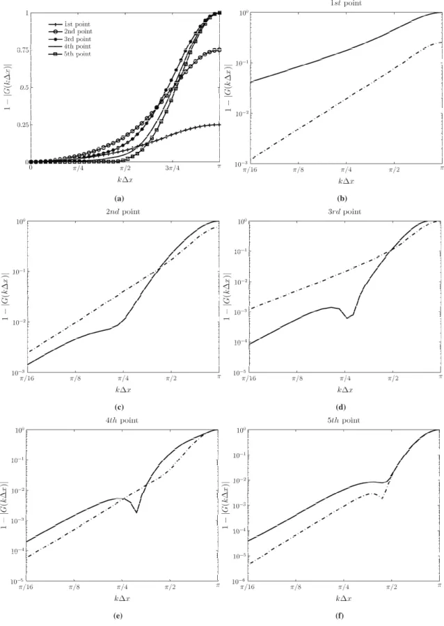
We now turn to an evaluation of the spectral properties of the 11-point conservative boundary filter in in Fig. 1. To this end, the dissipative properties of the filter are investigated, by displaying∥1−Gi(k∆x)∥in the five points closest to the boundary. As a point of reference, the boundary filters derived in [7] are also plotted (the coefficients are listed in Table A.10). It is appreciated that the dissipation of the filters in the low wavenumber range is kept at a very low level, which is required to allow for accurate CAA simulations while using the filter to removeπ-modes. As discussed above, for the conservative filters, theπ-mode constraint is not imposed in the first two grid points, and this is clearly visible in Fig. 1(b) and (c), where the dissipation level of the conservative filters does not reach one fork∆x=π. When comparing the selectivity of the new conservative filters with Berlandet al.original boundary filters, it is appreciated that the conservative filters performs remarkably well. Only in the second and third point, the conservative filters are less selective in the low-wavenumber range.
(a) (b)
(c) (d)
(e) (f)
Figure 1.Dissipation of the 11-point matching conservative filter, and the 11-point non-conservative boundary filter listed in Table A.10. (a) The dissipation of the conservative boundary filter, and (b)-(f) the comparison of the dissipation of the conservative filter and the non-conservative filter at the first five points from the wall. Solid line: the non-conservative filter (Table A.10); dashed line: conservative boundary filter.
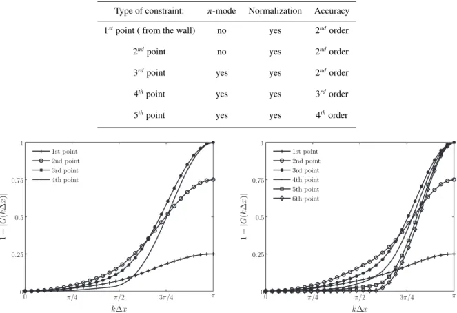
Table 1.The constraints imposed in each boundary point of the 11-point matching conservative boundary filter
Type of constraint: π-mode Normalization Accuracy 1stpoint ( from the wall) no yes 2ndorder
2ndpoint no yes 2ndorder
3rdpoint yes yes 2ndorder
4thpoint yes yes 3rdorder
5thpoint yes yes 4thorder
k∆x 1 − | G ( k ∆ x ) | 1st point 2nd point 3rd point 4th point 0 π/4 π/2 3π/4 π 0 0.25 0.5 0.75 1 k∆x 1 − | G ( k ∆ x ) | 1st point 2nd point 3rd point 4th point 5th point 6th point 0 π/4 π/2 3π/4 π 0 0.25 0.5 0.75 1
Figure 2.The dissipation of the 9-point (left) and 13-point (right) matching conservative boundary filters
Nine-point and 13-point matching conservative boundary filters are derived in a similar way. The dissipation level of these filters are shown in Fig. 2 and the coefficients of the 7-point, 9-point, 11-point, and 13-point matching conservative boundary filters are shown respectively in Table A.6, Table A.7, A.8, and A.9, provided in the appendix. To remove odd-even decoupling in practice, it is not always necessary to apply a low-pass filter at every time step in the simulations, and it may be sufficient to only use it everyntime steps, as already explained in§2.2. Moreover, it can also suffice to use the filter at reduced strength, i.e. constructing a filter velocity fieldevas
ev=(1−σ)v+σv=(1−σ)v+σGv, (27)
withσ≤1 the filter strength of the high-order low-pass filter used to removeπ-modes. Moreover, for the implemen-tation of the one-sided boundary filters in Ref. [7], Berlandet al.suggest to reduce the strength of the filter in the first point near the wall with a factor of 10 compared to the filter strength at other points, such that damping effects on large scales of the solution remain negligible (cf. Figure 1b, where Berland’s filter at the first point displays relative large damping at small wavenumbers, compared to the filters at next points). It should be also noted that the dissipation level of the conservative filters developed in this work at the first two boundary points is notably lower than that of
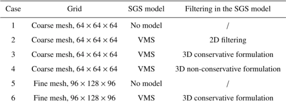
Table 2.Overview of channel flow test cases used to test the filtering of the VMS model
Case Grid SGS model Filtering in the SGS model 1 Coarse mesh, 64×64×64 No model /
2 Coarse mesh, 64×64×64 VMS 2D filtering 3 Coarse mesh, 64×64×64 VMS 3D conservative formulation 4 Coarse mesh, 64×64×64 VMS 3D non-conservative formulation 5 Fine mesh, 96×128×96 No model /
6 Fine mesh, 96×128×96 VMS 3D conservative formulation
other points. So there is no need to tune up the dissipation and the same filtering strength should used for all the filters to ensure the global conservation property.
4. Numerical results
We now turn to the evaluation of conservative boundary filters in simulations. First, in§4.1, channel-flow simula-tions are presented, and the effect of conservative filtering on VMS subgrid-scale modeling, and on removingπ-modes is elaborated. Next, in§4.2, 2D cavity simulations are presented, and the importance of conservative filtering for re-moval ofπ-modes is illustrated for the correct prediction of the flow pattern, and the corresponding cavity Strouhal number.
4.1. Channel flow
Large-eddy simulations of turbulent channel flow are performed, using a VMS Smagorinsky subgrid-scale model (cf.§2.1). The Reynolds number based on friction velocity,Reτ=300. The corresponding Reynolds number based on the mean stream-wise velocity is approximately 104. As a point of reference LES results are compared with the DNS data which are obtained from Ref. [21]. Simulations are conducted using the in-house compressible code FLOWAVE; the Mach number has been set to 0.2, such that the effect of compressibility is negligible.
In first instance, the effect of conservative filter formulations on the VMS Smagorinsky model is investigated (cf. also the discussion in§2.2). To construct the high-pass filter required for the VMS model, we either use the conservative low-pass top-hat filter of Vreman (cf. Eq. 17), or a standard non-conservative version discretized with the trapezoidal integration rule. An overview of the different simulations carried out to test the VMS filtering is given in Table 2. Two different grids are included (denoted as ‘coarse’ and ‘fine’). For the coarse mesh, four different cases are considered: (1) a no-model case, (2) a case with 2D wall-parallel filtering (as often used for channel-flow LES in the past), (3) a case with a 3D conservative formulation of the filtering, and (4) a non-conservative formulation (similar to the case discussed in Ref. [14]). For the coarse mesh, only a no-model simulation, and VMS using a conservative formulation of the filtering are performed.
y+ u + 100 101 102 0 5 10 15
a
y+ u + 100 150 200 16 17 18 19 y+ u + 100 101 102 0 5 10 15b
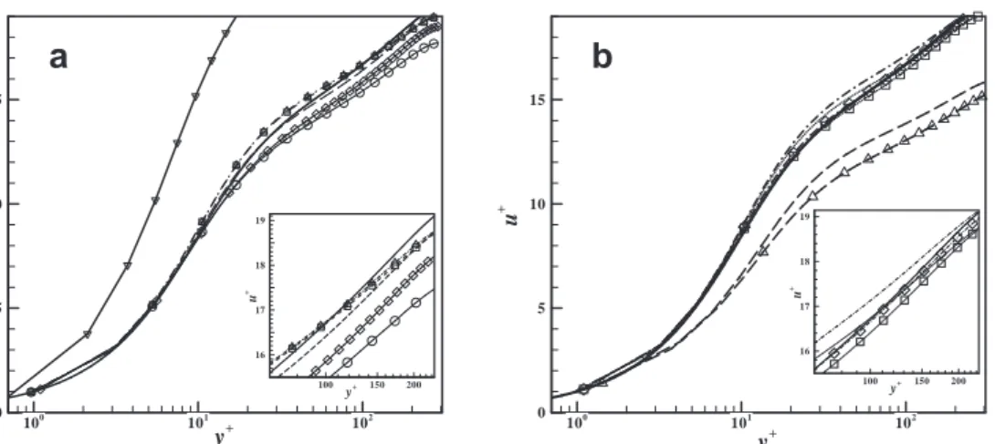
y+ u + 100 150 200 16 17 18 19Figure 3.Mean stream-wise velocities of the channel-flow testing. (a) Obtained by applying various conservative or non-conservative top-hat filters in the VMS model. (—): DNS refrence data [21]; (—⃝): no-model simulation on the coarse mesh; (—♢): no-model simulation on the fine mesh; (−−): LES simulation on the coarse mesh with filtering applied in wall-parallel directions; (− · △): LES simulation on the coarse mesh with conservative filtering applied in three directions; (—▽): LES simulation on the coarse mesh with non-conservative filtering applied in three directions; (−−): LES simulation on the fine mesh with conservative filtering applied in three directions. (b) Obtained by applying various high-order filters to remove grid-to-grid oscillations. (—): DNS refrence data; (· · ·): LES simulation on the coarse mesh without spatial filtering; (−−): LES simulation on the coarse mesh with the non-conservative filter in Table A.9; (− · △): LES simulation on the fine mesh with the non-conservative filter in Table A.9; (· · ·): LES simulation on the fine mesh without spatial filtering; (− −♢): LES simulation on the coarse mesh with conservative filters; (−·): LES simulation on the fine mesh with conservative filters.
In Figure 3a, the mean stream-wise velocity profiles are shown for the different cases listed in Table 2. The velocity is normalized using the friction velocity predicted by the LES simulations. It can be seen that the result obtained from the 3D non-conservative formulation deviates strongly from the DNS data. The velocity and friction velocity near the wall are not correctly predicted due to the failure of this formulation in satisfyingτM,w =0 (cf. discussion in§2.2), leading to a deviation which is even bigger than that of the no-model simulations. The result with the 3D conservative formulation of the VMS filters matches the DNS data very well, and also corresponds closely with results obtained using 2D filtering. It is appreciated that also on the coarse mesh, the 3D conservative formulation yields satisfactory results.
We now turn to the use of filters to remove odd-even decoupling or so-calledπ-modes. The use of top-hat filters is not appropriate for this, since they are not sufficiently selective in only removing theπ-modes, and not the large scales in the simulations. Hence, instead, we focus on the high-order conservative filters developed in§3, and use an 11-point filter to removeπ-modes in the simulations. For the subgrid-scale model, a VMS model with conservative formulation is used.
Several cases are considered. Apart from the new conservative filters, and a reference case without filtering, we also include different versions of Berland’s filter. The first version straightforwardly uses the one-sided filter
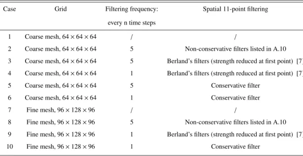
Table 3.Channel-flow cases used to test the use of spatial filters for removal of grid-to-grid oscillations
Case Grid Filtering frequency: Spatial 11-point filtering every n time steps
1 Coarse mesh, 64×64×64 / /
2 Coarse mesh, 64×64×64 5 Non-conservative filters listed in A.10 3 Coarse mesh, 64×64×64 5 Berland’s filters (strength reduced at first point) [7] 4 Coarse mesh, 64×64×64 1 Berland’s filters (strength reduced at first point) [7] 5 Coarse mesh, 64×64×64 5 Conservative filter
6 Coarse mesh, 64×64×64 1 Conservative filter
7 Fine mesh, 96×128×96 / /
8 Fine mesh, 96×128×96 5 Non-conservative filters listed in A.10 9 Fine mesh, 96×128×96 1 Berland’s filters (strength reduced at first point) [7] 10 Fine mesh, 96×128×96 1 Conservative filter
coefficients listed in Table A.10. In the second version, we follow Berland’s suggestion to reduce the strength of the filter in the first point (closest to the wall) with a factor of 10 compared to the other points, such that damping properties of the filter scheme near the wall are improved (although this filter is still non-conservative, good results were shown in Ref. [7]). A coarse and a fine grid are considered, i.e. 643, and 96×128×96, respectively. Finally the
filters are either applied every time step (n=1) or every 5 time steps (n=5), with an overall filter strength ofσ=0.25. Table 3 summarizes the test cases involved.
Looking at velocity fields for all test cases, we find that all filters are effective in removing grid-to-grid oscillations (results not shown here), even forn =5, andσ =0.25. We now focus on the quality of the predictions. First of all, we look at mean stream-wise velocity profiles in Figure 3b. Four cases are shown, i.e. the high-order conservative filter, the non-conservative filter as listed in Table A.10, both usingn =5, and applied on the coarse and on the fine mesh. It is appreciated that the use of non-conservative filter formulation seriously under-predicts the mean velocity; in contrast results of conservative filtering differ little from the DNS data.
Berland et al. [7] did not advocate the use of their filter as listed in Table A.10, but instead advised to reduce the strength of the filter at the first point. To further assess this, an overview of errors on the predicted friction velocity, and center velocity is presented in Table 4 for all cases, including Berland’s filter with reduced near-wall strength. It is appreciated that errors of the non-conservative filter (Table 4) are very large, in particular on the prediction of the friction velocity. When using Berland’s filter with reduced strength near the wall, it is appreciated that results may be accurate, in particular for the first case listed in the table. However, when changing the frequency at which the filter is applied (n), we find larger errors, even when the mesh is refined. For the conservative filters, accurate results are found independent of mesh size and filter frequency.
Table 4.Errors induced by use of the conservative filter, and different non-conservative filters Filter Mesh n error on mass-flow rate error on friction velocity
non-conservative (Table A.9) coarse 5 4% 27%
fine 5 5% 30%
Berland’s filter [7] coarse 5 2.3% 2.4%
(strength reduced coarse 1 4.3% 10.9%
at first point) fine 1 2.6% 11.3%
conservative filter coarse 5 2.4% 0.3%
coarse 1 3.4% 0.3%
fine 1 3.4% 0.5%
In the current channel-flow simulations, the computational grid is stretched in the wall normal direction. with maximum stretching ratios of 10.5% and 3.2% for the coarse mesh and the fine mesh respectively. For the imple-mentation of the conservative filter, we did not take this stretching into account, but straightforwardly use the filters derived in§3. Hence, on these stretched grids, these filters are formally not conservative, but we found the errors to be small, as listed in Table 4. It is appreciated that even for a rather high stretching ratio of 10% on the coarse grid, the error induced on the friction velocity by using the conservative filters on stretched grids remains small (<0.5%). The error on the mass-flow rate is a bit higher, but this is not related to the conservation properties of the filter, but rather to errors in the subgrid-scale closure, and the discretization in the bulk of the flow.
4.2. 2D cavity flow
We now turn to a 2D cavity flow, and investigate the possible influence of the filter formulation for removing
π-modes, on noise predictions. The noise radiated by flow passing over cavities has been studied extensively in the past [23, 26, 27], is connected to a broad range of aerospace and automotive applications, and a variety of theoretical questions on noise production. The spectrum of cavity noise contains both broadband components introduced by the turbulence in the shear layer, and tonal components. The mechanisms for the intense tonal components in cavities have been identified and can be either [26]
1. a shear-layer mode mechanism in which the shear-layer generated at the upstream edge of the cavity impinges on the rear edge of the cavity, scattering acoustic waves that propagate upstream and further excite the shear layer, or
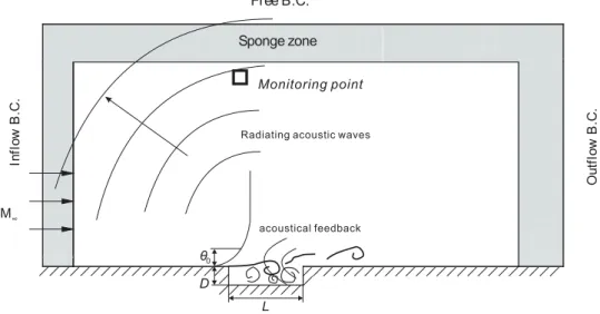
M∞ Sponge zone O u tf lo w B .C . Fr B.C. In fl o w B .C . e e L D 0 θ
Radiating acoustic waves
acoustical feedback
Monitoring point
Figure 4.Cavity configuration.
In the current simulations, we focus on the shear-layer mode. Frequency of tonal noise in the shear-layer mode can be estimated by an empirical expression, originally introduced by Rossiter [25]:
St= f L U∞ =
n−α
M+1/κ (28)
whereSt(Strouhal number) is the dimensionless frequency, f is the frequency, Lis the length of the cavity,U∞is free stream velocity, n is the mode number,M is undisturbed Mach number,κ andαare empirical constants. The values forκandαare obtained experimentally and equal to 0.57 and 0.25 respectively for the cavity studied in present research.
We consider a 2D cavity corresponding to the DNS cavity case of Gloerfelt [23]. The configuration of the cavity is shown in Figure 4. Its length-to-depth ratio isL/D = 4, and the free-stream Mach number is M = 0.5. The Reynolds number based on the depth of the cavity corresponds to 4800 and the ratioL/θ=63, whereθis the initial boundary layer momentum thickness at the leading edge of the cavity. The sound field in this flow is dominated by the shear-layer mode which generates the dominant modes in the noise spectrum.
In the current study, simulations with two different grids are included. A coarse mesh uses 101×51 points inside the cavity and 379×121 outside; a finer mesh uses 201×51 points inside the cavity and 679×221 outside. The computational domain extends over 13D vertically and 28D horizontally to include a portion of the radiated field. At the inlet, three velocity components and temperature are specified; at the outlet, the pressure is imposed. A free boundary condition is applied at the top boundary. In order to reduce spurious wave reflection at the outer boundaries, sponge zones are included at all boundaries, by using progressive damping terms towards the hard boundary of the mesh. To removeπ-modes in the simulations, either the 11-point conservative filter, or a non-conservative filter [7] (cf. Table A.10) are used at the final Runge–Kutta stage of every iteration. Here, we use the latter filter as a reference to illustrate potential errors of non-conservative filters on noise prediction (for the current case, we do not further include
Berland’s filter with reduced strength near the wall, though these may obviously yield better results, depending on mesh size and filter frequency, i.e. cf.§4.1). Simulations start from a Blasius laminar boundary layer along the wall and spanning the cavity. Computations are first run for a few hundred dimensionless time units until the oscillations in the shear layer are established. Subsequently, averaging in time is used over a sufficiently long time window for averaged quantities to statistically converge.
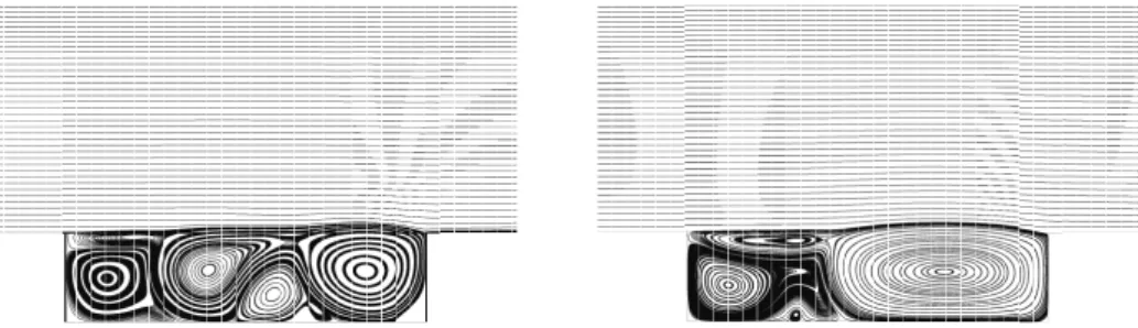
Figure 5 and 6 respectively show two instantaneous vorticity fields and pressure fields in one cycle of the domi-nant Rositer mode, obtained using an 11-point conservative filter (left), and a non-conservative filter (cf. Table A.10) (right), both obtained on the fine mesh. It is appreciated that large differences exist between solutions obtained with both filter formulations. The structure of the conservative solution very much resemble the flow patterns found in the work of Gloerfelt [23, 24] associated to the shear-layer mode of the cavity. To further investigate the difference be-tween solutions using either conservative or non-conservative filtering, streamlines associated with the time-averaged solution of both cases are presented in Figure 7. It is appreciated that large differences exist; in particular the non-conservative case displays a big stationary vortex occupying the rear part of the cavity, which is more reminiscent of a wake-like cavity mode than of a shear-layer mode.
In Figure 8 we investigate grid dependency of the solutions for both filter types, by looking at the pressure co-efficient along the bottom cavity wall for the coarse and fine mesh. We find that the pressure coefficients for the conservative filters coincide for both grids (the respective lines are not distinguishable on the plot), and trends corre-spond well with pressure coefficients reported in the literature [23, 24]. The results of the non-conservative filters show a large variation when the grid is refined. For the finer grid, it is observed that the results using the non-conservative filters (Table A.10) start approaching the solution found with conservative filters. This trend is to be expected, since even though the these filters are non-conservative, they still provide a consistent discretization of the governing equa-tions, such that continued grid-refinement should eventually lead to an exact solution. However, it is appreciated for the current case, that much finer grid levels will be needed for this.
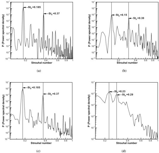
In order to identify the dominant tonal frequencies of the noise, time signals are recorded at a point above the cavity with co-ordinate (0.2D,10D) (with respect to the leading edge of the cavity. See also Figure 4). Figure 9 shows the power spectral density of the fluctuating pressure recorded at the monitoring point for the different cases. The results obtained with the conservative filters display consistent features for both the coarse mesh and fine mesh, with dominant frequencies atSt=0.185, which is very close to the first Rossiter modeSt=0.19. This is also in line with the results reported in [23, 24] based on DNS. When looking at the results obtained with non-conservative filters, it is appreciated that the dominant frequencies depends strongly on the grid, and corresponds toSt=0.15 andSt=0.23 for the coarse and fine grid.
Figure 5.Vorticity fields during one cycle of oscillation (First Rossiter mode) obtained by the 11-point conservative filters (left) and non-conservative filters (right) on the fine mesh.
Figure 6.Pressure contours during one cycle of oscillation (First Rossiter mode) obtained by the 11-point conservative filters (left) and non-conservative filters (right) on the fine mesh.
Figure 7.Time avaraged streamlines on the fine mesh by the conservative filter (left) and non-conservative filter (right).
Figure 8.Mean pressure coefficient along the cavity bottom wall obtained by (—–): the fine mesh and conservative filter, (—–
): the fine mesh and non-conservative filter (Table A.10), (– –): the coarse mesh and conservative filter, (– –): the coarse mesh and non-conservative filter.
5. Conclusion
Globally conservative high-order filters were elaborated and used for LES simulations. Focus is on selective filters for removing grid-to-grid oscillation in simulations. Nine-, eleven-, and thirteen-point stencils, and associated one-sided boundary schemes, were elaborated. Next to that, the importance of a conservative filter formulation for use in the VMS Smagorinsky subgrid-scale model was also highlighted.
In a first step, the conservative filter was tested in channel-flow LES, and comparisons with simulations using non-conservative filters were presented. When using these filters to removeπ-modes, it was demonstrated that a conservative 11-point stencils leads to accurate results both on coarse and finer grids. When using a non-conservative formulation, large errors on the prediction of the skin friction were detected. We used the channel-flow test case also to test the effect of a conservative filter formulation in the formulation of the Smagorinsky model. Here, the use of a conservative top-hat filter, as proposed by Vreman [8], was compared to a traditional top-hat implementation. Again, we found that non-conservative formulations can lead to large errors; in this case errors up to 10% on the prediction of the friction velocity.
-Strouhal number P (P o w e r s p e c tr a l d e n s it y ) 0.2 0.4 0.6 0.8 1 10-10 10-9 10-8 10-7 10-6 10-5 10-4 10-3 10-2 10-1 StD=0.37 StD=0.185 (a) Strouhal number P (P o w e r s p e c tr a l d e n s it y ) 0.2 0.4 0.6 0.8 1 10-10 10-9 10-8 10-7 10-6 10-5 10-4 10-3 10-2 10-1 StD=0.30 StD=0.15 (b) Strouhal number P (P o w e r s p e c tr a l d e n s it y ) 0.2 0.4 0.6 0.8 1 10-10 10-9 10-8 10-7 10-6 10-5 10-4 10-3 10-2 10-1 StD=0.37 StD=0.185 (c) Strouhal number P (P o w e r s p e c tr a l d e n s it y ) 0.2 0.4 0.6 0.8 1 10-8 10-7 10-6 10-5 10-4 10-3 StD=0.29 StD=0.23 (d)
Figure 9.Power spectral density of fluctuating pressure versus the Strouhal numberS t=f L/U∞at the position (0.2D,10D) by: fine mesh with conservative filter (a); fine mesh with non-conservative filter (b); coarse mesh with conservative filters (c); coarse mesh with non-conservative filter (d).
modes, on noise predictions in aero-acoustics applications, simulations of a 2D cavity flow were conducted. It was observed that simulations with the conservative boundary filters captured the flow pattern of shear-layer mode and the dominant frequencies correctly, while the simulations with non-conservative filter formulation failed to do so. It was observed for the non-conservative filters, that the flow structure near the boundaries is significantly changed, leading to entirely different recirculation patterns inside the cavity.
Acknowledgment
This research was performed in the framework of the SBO-CAPRICORN project sponsored by the Flanders Institute for Innovation and Technology (IWT – Vlaanderen). The authors would like to express their gratitude for the financial support by IWT. The authors alos gratefully acknowledge Christophe Bogey and Xavier Gloerfelt for useful discussions on spatial high-order filters and the 2D cavity case respectively.
Appendix A. Coefficients of 9-, 11-, and 13-point conservative boundary filters
j 1 2 3 4 g0 0.287392842460 0.24352749312000 0.23481047976170 0.19089951150600 g1 -0.226146951809 -0.20478888064000 -0.19925013128581 -0.17150383223600 g2 0.106303578770 0.12000759168000 0.12019831024519 0.12363289179700 g3 -0.023853048191 -0.04521111936000 -0.04930377563602 -0.06997542910500 g4 0.00822866176000 0.01239644987396 0.02966275473600 g5 -0.00144609307817 -0.00852073865900 g6 0.00125459771400
Table A.5.The 7-point [28], 9-point [6], 11-point [29] and 13-point [6] spatial filters for internal points,g−j=gj
j 1 2 3 b1,j 0.04254946942100 -0.10374863021700 0.08505220898700 b2,j -0.10374863021700 0.27129809963800 -0.250000000000000 b3,j 0.08505220898700 -0.25000000000000 0.30864421224300 g4−j -0.02385304819100 0.10630357877000 -0.22614695180900 g5−j -0.0238530481910 0.10630357877000 g6−j -0.02385304819100
j 1 2 3 4 b1,j 0.04197486592000 -0.09624620416000 0.07479647232000 -0.02875379584000 b2,j -0.09624620416000 0.24676374656000 -0.23354267648000 0.12000759168000 b3,j 0.07479647232000 -0.23354267648000 0.29696727424000 -0.22124620416000 b4,j -0.02875379584000 0.12000759168000 -0.22124620416000 0.25175615488000 g5−j 0.00822866176000 -0.04521111936000 0.12000759168000 -0.20478888064000 g6−j 0.00822866176000 -0.04521111936000 0.12000759168000 g7−j 0.00822866176000 -0.04521111936000 g8−j 0.00822866176000
Table A.7.The coefficients of the 9-point matching conservative boundary filters
j 1 2 3 4 5 b1,j 0.04170901551687 -0.09759693795557 0.07523281384367 -0.02595696896626 0.00805817063946 b2,j -0.09759693795557 0.24818961219352 -0.22954537948657 0.11441393793252 -0.04641158947969 b3,j 0.07523281384367 -0.22954537948657 0.28928023988085 -0.21970475179924 0.12309049640152 b4,j -0.02595696896626 0.11441393793252 -0.21970475179924 0.25299130194833 -0.20358841052031 b5,j 0.00805817063946 -0.04641158947969 0.12309049640152 -0.20358841052031 0.23625657283987 g6−j -0.00144609307817 0.01239644987396 -0.04930377563602 0.12019831024519 -0.19925013128581 g7−j -0.00144609307817 0.01239644987396 -0.04930377563602 0.12019831024519 g8−j -0.00144609307817 0.01239644987396 -0.04930377563602 g9−j -0.00144609307817 0.01239644987396 g10−j -0.00144609307817
Table A.8.The coefficients of the 11-point matching conservative boundary filters
j 1 2 3 4 5 6 b1,j 0.04031416306317 -0.09321174458200 0.07147004890233 -0.02692028815167 0.01196119032050 -0.00486796726633 b2,j -0.09321174458200 0.23345995106884 -0.21306138057267 0.11279882665300 -0.06020613618633 0.02748662456417 b3,j 0.07147004890233 -0.21306138057267 0.26254508756000 -0.20571121271533 0.13506751108767 -0.07270666805300 b4,j -0.02692028815167 0.11279882665300 -0.20571121271533 0.22910917945267 -0.18887233136900 0.12717464144433 b5,j 0.01196119032050 -0.06020613618633 0.13506751108767 -0.18887233136900 0.19842105434483 -0.17242536468067 b6,j -0.00486796726633 0.02748662456417 -0.07270666805300 0.12717464144433 -0.17242536468067 0.19078848974450 g7−j 0.00125459771400 -0.00852073865900 0.02966275473600 -0.06997542910500 0.12363289179700 -0.17150383223600 g8−j 0.00125459771400 -0.00852073865900 0.02966275473600 -0.06997542910500 0.12363289179700 g9−j 0.00125459771400 -0.00852073865900 0.02966275473600 -0.06997542910500 g10−j 0.00125459771400 -0.00852073865900 0.02966275473600 g11−j 0.00125459771400 -0.00852073865900 g12−j 0.00125459771400
Table A.9.The coefficients of the 13-point matching conservative boundary filters
j 1 2 3 4 5 6 b1,j 0.320882352941 -0.085777408969 0.07147004890233 0.0307159855992469 0.01196119032050 0.008391235145 b2,j -0.465 0.277628171524 -0.21306138057267 -0.148395705486028 -0.06020613618633 -0.047402506444 b3,j 0.179117647059 -0.356848072173 0.26254508756000 0.312055385963757 0.13506751108767 0.121438547725 b4,j -0.035 0.223119093072 -0.20571121271533 -0.363202245195514 -0.18887233136900 -0.200063042812 b5,j -0.057347064865 0.13506751108767 0.230145457063431 0.19842105434483 0.240069047836 b6,j -0.000747264596 -0.07270666805300 -0.0412316564605079 -0.17242536468067 -0.207269200141 b7,j -0.000027453993 0.02966275473600 -0.0531024700805787 0.12363289179700 0.122263107843 b8,j 0.0494343261171287 -0.06997542910500 -0.047121062819 b9,j -0.0198143585458560 0.02966275473600 0.009014891495 b10,j 0.00339528102492129 -0.00852073865900 0.001855812216 b11,j 0.00125459771400 -0.001176830044
Table A.10.The coefficients of the 11-point matching boundary filters derived in Ref. [7]
[1] C. Wagner, T. H¨uttl, P. Sagaut,Large-Eddy Simulation for Acoustics, Cambridge University Press, 2007.
[2] C. K. W. Tam, J. C. Webb, Dispersion-relation-preserving finite difference schemes for computational acoustics,J. Comput. Phys. 107, 1993, 262.
[3] S. K. Lele, Compact finite difference schemes with spectral-like resolution,J. Comput. Phys. 103, 1992, 16.
[4] C. K. W. Tam, J. C. Webb, Z. Dong, A study of the short wave components in computational acoustics,J. Comput. Ac. 1, 1993, 2012. [5] C. K. W. Tam, H. Shen, Direct computation of nonlinear acoustic pulses using high order finite difference schemes,AIAA Paper 93-4325,
1993.
[6] C. Bogey, C. Bailly, A family of low dispersive and low dissipative explicit schemes for flow and noise computations,J. Comput. Phys. 194, 2004, 194.
[7] J. Berland, C. Bogey, O. Marsden, C. Bailly, High-order, low dispersive and low dissipative explicit schemes for multiple-scale and boundary problems,J. Comput. Phys. 224, 2007, 637.
[8] A. W. Vreman, The adjoint filter operator in large-eddy simulation of turbulent flow,Phys. Fluids 16, 2004, 2012.
[9] J. R. Hughes, A. A. Oberai, L. Mazzei, Large eddy simulation of turbulent channel flows by the variational multiscale method,Phys. Fluids 13, 2001, 1784.
[10] J. R. Hughes, L. Mazzei, K. E. Jansen, Large eddy simulation of turbulent channel flows by the variational multiscale method,Comput. Visualization Sci. 3, 2000, 47.
[11] A. W. Vreman, The filtering analog of the variational multiscale method in large-eddy simulation,Phys. Fluids 15, 2003, L61.
[12] H. Jeanmart, G. Winckelmans, Investigation of eddy-viscosity models modified using discrete filters: A simplified regularized variational multiscale model and an enhanced field model,Phys. Fluids 19, 2007, 055110.
[13] J. Meyers, P. Sagaut, Evaluation of Smagorinsky variants in large-eddy simulations of wall-resolved plane channel flows,Phys. Fluids 19, 2007, 095105.
[14] S. Stolz, P. Schlatter, L. Kleiser, High-pass filtered eddy-viscosity models for large-eddy simulations of transitional and turbulent flow,Phys. Fluids 17, 2005, 065103.
[15] P. Sagaut,Large Eddy Simulations for Incompressible flows, Springer, Berlin, third ed., 2006. [16] B. J. Geurts,Elements of Direct and Large-Edddy Simulation, Edwards, Flourtown, 2003.
[17] R. Cocle, L. Bricteux, D. Winckelmans, Scale dependence and asymptotic very high Reynolds number spectral behavior of multiscale subgrid models,Phys. Fluids 21, 2009, 085101.
[18] J. Meyers, P. Sagaut, On the model coefficients for the standard and the variational multi-scale Smagorinsky model,J. Fluid Mech. 596, 2006, 287.
[19] O. Marsden, C. Bogey, C. Bailly, High-order curvilinear simulations of flows around non-Cartesian bodies,J. Comput. Ac. 13, 2005, 731. [20] S. B. Pope,Turbulent Flows, Cambridge University Press, 2000.
[21] K. Iwamoto, Y. Suzuki, N. Kasagi, Reynolds number effect on wall turbulence: toward effective feedback control,Int. J. Heat Fluid Flow 23, 2000, 678.
[22] O. V. Vasilyev, T. S. Lund, P. Moin, A general class of commutative filters for LES in complex geometries,J. Comput. Phys. 146, 1998, 82. [23] X. Gloerfelt, C. Bailly, D. Juv´e, Calcul direct du rayonnement acoustique d’un ´ecoulement affleurant une cavit´e,C. R. Acad. Sci, S´erie 328(8),
2000, 625.
[24] X. Gloerfelt,Bruit rayonne par un ecoulement affleurant une cavite: simulation aeroacoustique directe et application de methodes integrales, Ph.D. thesis, ´Ecole Centrale de Lyon, 2001.
[25] J. E. Rossiter,Wind tunnel experiments on the flow over rectangular cavities at subsonic and transonic speeds, Technical report 64037, Royal Aircraft Stablishment, 1964.
[26] C. W. Rowley,Modeling, simulation, and control of cavity flow oscillations, Ph.D. thesis, California Institute of Technology, 2002. [27] K. Takeda, CM. Shieh, Cavity tones by computational aeroacoustics,Int. J. Comput. Fluid. D. 228, 2004, 439.
[28] C. K. W. Tam, Computational aeroacoustics: issues and methods,AIAA Journal 33, 1995, 1788.
[29] C. Bogey, N. de Cacqueray, C. Bailly, A shock-capturing methodology based on adaptative spatial filtering for high-order non-linear compu-tations,Journal of Computational Physics 228(5), 2009, 1447-1465