A Study of Time Series Model for Forecasting of Boot in Shoe
Industry
Amrit Pal singh
*, Manoj Kumar Gaur, Dinesh KumarKasdekar and Sharad
Agrawal
Department of Mechanical Engineering, Madhya Institute of Technology &
Science, Gwalior, INDIA
*
Corresponding Author e-mail:[email protected]
Abstract
Predicting sales in a shoe industry is a typical job due to unpredictable demand of products. Many models are suggested for forecasting the product in the literature over the past few decades. Most shoe manufacturing organizations are in a continuous effort for increasing their profits and reducing their costs. Exact sales forecasting is certainly an inexpensive way to meet the organization goals. This paper studies and compares different forecasting techniques as moving average, single exponential smoothing, double exponential smoothing and winter’s method. For this, domestic sales data from a shoe industry is collected and then data were analyzed by statistics technique using Minitab 17 software. The result shows that the demand of shoes fluctuate over the period of time. The factor that influences the choice of forecasting model is the least value of Mean square deviation (MSD).
Keywords: time-series, sales forecasting, shoe product, MSD
1. Introduction
Industry forecasts are mainly useful to big retailers who might have a superior market share. For the retailing industry, R. T. Peterson [1] showed that larger retailers are more likely to use time-series methods and prepare industry forecasts, while smaller retailers give importance to judgmental methods and company forecasts. Predicting sales accurately in the shoe industry is generally considered challenging due to volatile demand of products. Regardless of the known difficulties, predicting sales in the industry is considered to be crucial due to the long lead times caused by the relatively current trend of sourcing production and operations to other countries. The interesting concept of predicting sales, more commonly referred to as demand or sales forecasting, in the swiftly changing industry has been greatly researched in the past decades. This has resulted in a large number of published forecasting ideas, methods and measures aiming to produce as exactly predicted demand as possible while admitting that an error-free forecast is never possible. The varieties of ideas available, together with the generally large forecasting errors, have made the process of choosing a valid forecasting method and applying it in a suitable manner for the companies.
Tej international group produce and export the best quality footwear all over the world by manufacturing broad range of comfort, casual and business shoes. All the Factories are established in vast spaces and prepared with state-of-the-art machines includes a variety of fully Mechanized conveyor systems with on line quality check at every stage throughout the production. The shoes come with the finest quality of material used in soles like Polyurethane(PU), Thermoplastic rubber(TPR), Thermo Polyurethane (TPU) and Polyvinyl chloride (PVC). (Injection Footwear 3000 Pairs per day, Hand-Stiched and San Crispino Footwear 7000 Pairs per day, Cemented Footwear 5000 Pairs per day). This paper studies and compares different forecasting techniques, moving average, single
exponential smoothing, double exponential smoothing, and winter’s method. All the forecasting technique applied to the same real data that have varied intermittent demand.
2. Literature Review
H. K.
Alfares
& M.Nazeeruddin
[2] categorized the electric load forecasting technique. A wide range methodologies and model for forecasting are given in literature. These technique are classified into nine categories: (1) multiple regression, (2) exponential smoothing, (3) iterative reweighted least squares, (4) adaptive load forecasting, (5) stochastic time series, (6) ARMAX model based on genetic algorithms, (7) fuzzy logic, (8) neural networks and (9) expert systems. The methodology for each category is briefly described, the advantage and disadvantages discussed. W. Peter & S.Anders
[3] developed flexible and robust supply chain forecasting systems under changing market loads. They suggested new tools and models to estimate forecasting error measurements. The paper mainly studies slow moving or intermittent demand, when for items the forecasting time periods over and over again have zero demand. For the difficult to forecast intermittent demand the Croston forecasting technique is mostly regarded as a better alternative than single exponential smoothing. These two methods, Croston and single exponential smoothing, mutually with two modifications of the Croston method, are discussed and evaluated with real intermittent data. The held performance of a forecasting technique is dependent of the chosen measurement of forecast errors. The main purpose is to examine and estimate different forecasting error measurements. C.Cacatto
, P.Belfiore
& J. G. V.Vieira
[4] introduced the forecasting practices that have been used by food industries in Brazil and detected how these companies use forecasting methods and what the main factors that influence their selection. The data were analyzed by multivariate statistics techniques using the SPSS software. They stated that the companies did not use sophisticated forecasting methods, the historical analysis model was the mostly used. The factors that influence the choice of the models are the type of product and the time spent during the forecasting. M.Sanwlani
& M.
Vijayalakshmi
[5] studied the effect of decomposing time series into multiple components like trend, seasonal and irregular and performed the clustering on those components and generate the forecast values of each component separately, they worked on sales data. Statistical method ARIMA, Holt winter and exponential smoothing are used to forecast those components. Selection of best, good and bad forecasters are performed on the basis of count and rank of expert id’s generated, finally absolute percentage error (APE) is used for comparing forecast.D. P. Patil, A. P.
Shrotri
& A. R.Dandekar
[6] analyzed the advantage and disadvantage of basic, in-between and advanced method for visitor use forecasting where seasonality and limited data are characteristics of the assessment problem. Forecasting method include the naϊve model 1 and 2, moving average method, double moving method, exponential smoothing method, double exponential method, Holt’s method, Winter method and seasonal autoregressive integrated moving average (SARIMA) are used Milwaukee county zoo visitor forecasting A. K. Sharma, A. Gupta & U. Sharma [7]. The series ranged from January 1981 to 1999 or a total of 228 months. The last 12, 24 or 60 month of those data were excluded from the original analysis and they were used to evaluate the various methods. SARIMA and SMA with classical decomposition procedure were found to be roughly equivalent in performance, as judged by modified mean absolute percentage error method and modified root mean squared error value of longer estimation period with shorter period ahead forecasts. This study also found that the SMA with classical decomposition method was more accurate than other technique when shorter estimation period with longer period ahead forecast are included. C. D.Ezeliora
[8] analyzed the forecasting of plastic yield in Finoplastika manufacturing industry by using moving average analysis. They gathered the data of daily plastic pipe production
over the month for three years. They fitted moving average model to predict the product total, as the coefficient of determination shows a strong relationship. This model proposed optimum monthly production output for different products. K. Ryu & A.
Sanchez
[9] evaluated the forecasting method for institutional food service facility. They are identifying the most appropriate forecasting method of forecasting meal count for an institutional food service facility. The forecasting method analyzed included: naϊve model 1,2 and 3; moving average method, double moving method, exponential smoothing method, double exponential method, Holt’s method, Winter method, linear regression and multiple regression method. The accuracy of forecasting methods was measured using mean absolute deviation, mean squared error, mean percentage error, mean absolute percentage error method, root mean squared error and Theil’s Ustatistic. The result of this study showed that multiple regressions was the most accurate forecasting method, but naϊve method 2 was selected as the most appropriate forecasting method because of its simplicity and high level of accuracy. E.Leve'n & A. Segerstedt
[10] suggested a modification of the Croston method where a demand rate is directly calculated when a demand has happened. A. A.Syntetos
& J. E.Boylan
[11] recommended an adjustment of the Croston method due to a systematic error. J. J.Strasheim
[13] introduced variety of alternative forecasting techniques and they were evaluated for purpose of stock replenishment is an important function of part in the typical reordering motor vehicle spare parts with aim of selecting one optimal technique to be implemented in automatic reordering module of real time computerized inventory management system. A large number of forecasting technique wereevaluated, namely simple moving average(Averages, Moving Averages, Double Moving Averages),Exponential Smoothing(Single Exponential Smoothing, Adaptive Exponential Smoothing, DoubleExponential Smoothing (Brown's one 'parameter linear method and Holt's two parameter method),Triple Exponential Smoothing (Brown's one parameter quadratic method and Winter's threeparameter trend and seasonality method), linear Regression, Multiple Regression. The accuracy offorecasting methods was measured using statistical measures (mean error, mean absolute deviation, mean squared error), relative measures (percentage error, mean percentage error, mean absolutepercentage error method) and others measures (Theil’s U- statistic, Durban- Watson value and forecasting index).3. Data Collection
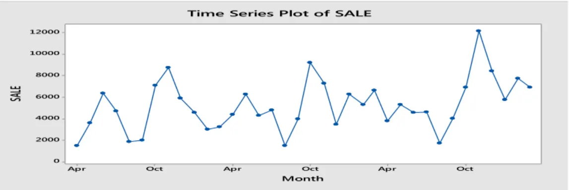
The data in this study has been collected from Tez international, Agra on monthly basis over a period of three years (April 2012 to March 2015). The domestic sales data of a product named army boot (Article number 741) has been taken and forecasting models are successively applied and then analyzed using statistical technique. Figure 1 shows last three years data starting from April 2012 to March 2015, the original data has been converted into graphical form using Minitab 17.
Figure 1. Time Series Plot of Sale
Oct Apr Oct Apr Oct Apr 12000 10000 8000 6000 4000 2000 0 Month SAL E
4. Methodology
Uncertainty in demand of product can be reduced through forecasting methods. There are various forecasting model used in the analysis, included simple moving average method, single exponential method , double exponential method(Holt’s), winter’s method. The most appropriate forecasting method was determined on the basis of accuracy. In this work, several common accuracy methods were used: Mean Absolute Deviation (MAD), Mean Absolute Percentage Error (MAPE), and Mean Square Deviation (MSD). In every method different numbers of trials have been used, out of which the best one (least MSD) is taken and plotted in graph.
4.1. Forecasting Methods 4.1.1. Moving Average Method
The moving average method involves calculating the average of observations and then employing that average as the predictor for the next period. The moving average method is highly dependent on n, the number of terms selected for constructing the average C.
Floros [14]
and S.Chopra
& P.Meindl
[15] the equation is as follows:1 2 1 1 ( Yt t t . . . t n ) t Y Y Y F n (1) Where:
Ft+1 = the forecast value for the next period,
Yt= the actual value at period t,
n = the number of term in the moving average. 4.1.2. Single Exponential Smoothing Method
The exponential smoothing method is a technique that uses weighted moving average of past data as the basis for a forecast. This method keeps a running average of demand and adjusts it for each period in proportion to the difference between the latest actual demand figure and the latest value of the average. The equation for the simple exponential smoothing method is:
1 ( 1 1)
t t t t
F F A F
(2)
Where:
Ft+1 = the new smoothing value or the forecast value for the next period,
α= the smoothing constant (0 < α <1),
Yt= the new observation or actual value of the series in period t,
Ft= the old smoothed value or forecast for period t.
4.1.3. Double Exponential Smoothing Method (Holt’s method)
The double exponential smoothing model is recommended to forecast time series data that have a linear trend P. Y Lim & C. V. Nayar [16]. An approach used to handle a linear trend is called the Holt’s two parameter method. Theoretically, this methodology is similar to Brown’s exponential smoothing, except that the technique smoothes the trend and the slope in the time series by using different smoothing constants for each. Low values of α and β should be used when there are frequent random fluctuations in the data, and high values when there is a pattern such as a linear trend in the data. Three equations are employed:
Tt= β(At− At − 1) + (1 − β )Tt– 1
Yt+ x= At+ xTt (3) Where:
At = smoothed value
α = smoothing constant (0 <α < 1)
β = smoothing constant for trend estimate (0 <β < 1)
Tt= trend estimate
x = periods to be forecast into future
Yt+x = forecast for x periods into the future
4.1.4. Winter’s Method
Winter’s method provides a useful way to explain the seasonality when time series data have a seasonal pattern. The formula of this method includes four equations:
At = αYt / It-L + (1-α)(At-1 + Tt-1) Tt = β(At - At-1 ) + (1-β) Tt-1 It = γYt / At + (1-γ) It-L
And to forecast p period into the future, we have:
Ft+p= (At + pTt )It-L+p (4)
Where:
At= smoothed value
α = smoothing constant (0<α <1)
Yt= actual value or new observation in period t
β = smoothing constant for trend estimate (0<β <1)
Tt= trend estimate
γ = smoothing constant for seasonality (0<γ <1)
It= seasonal estimate measured as an index
L = length of seasonality
p = periods to be forecast into future
Ft+p= the forecast for p periods into the future.
4.2. Measuring Forecasting Error
There is no consensus among researcher as to which measure is best for determining the most appropriate forecasting method. Accuracy is the criterion that determines the best forecasting method; thus, accuracy is the most important concern in evaluating the quality of a forecast. The goal of the forecasts is to minimize error. Forecast error is the difference between an actual value and its forecast value J. S.
Armstrong
& F.Collopy
[17]. Some of the common indicators used evaluate accuracy are mean forecast error, mean absolute deviation, mean squared error, and root mean squared error. Regardless of the measure being used, the lowest value generated indicates the most accurate forecasting model.
4.2.1. Mean Absolute Deviation
A common method for measuring overall forecast error is the mean absolute deviation (MAD). The value is computed by dividing the sum of the absolute values of the individual forecast error by the sample size (the number of forecast periods). The equation is: t t 1 ( Y F ) n t M A D n
Where:
Yt= the actual value in time period t,
Ft = the forecast value in time period t,
n = the number of periods. 4.2.2. Mean Square Deviation
The mean square error (MSD) is a generally accepted technique for evaluating exponential smoothing and other methods. The equation is:
2 t t 1 1 ( Y F ) n t M S D n
Where:Yt= the actual value in time period t,
Ft = the forecast value in time period t,
n = the number of periods.
4.2.3. Mean Absolute Percentage Error
Forecasters also depend on mean absolute percentage error (MAPE) as a measure of accuracy of a forecast. This measure is similar to MAD except that it is expressed in percentage terms. The advantage of the measure is that it takes into account the relative size of the error term to actual units of observation. Symbolically, the equation is:
1 | ( / ) .1 0 0 | n t t t e Y M A P E n
Where:Yt= the actual value in time period t,
et= the prediction error in time period t,
n = the number of periods.
5. Result and Discussion
The purpose of this work was to identify an appropriate forecasting method for boot product in Tez International, Agra Shoe Industry. Forecasting of boot production is a very important because sales vary in special festival and weather change. In this Research work, four forecasting methods namely-moving average, single exponential, double exponential and winters method are used. The most appropriate forecasting method was determined on the basis of accuracy. Mean absolute deviation (MAD), Mean absolute percentage error (MAPE) and Mean square deviation (MSD) were adopted to estimate the accuracy of forecasting methods. The lesser the forecasting error, the more accurate forecasting method. Forecasting of each method in tabular and plotted form is given below.
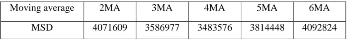
In simple moving average method, five trials were taken and different values of n are put in the equation (1). Least value of mean square deviation (MSD) is obtained at n=4 as given in Table 1. The optimal n value can be determined by interactive model to obtain the smallest error. In the above model, five experiments were conducted in which the optimal value is obtained at 4MA.
Table 1. Different Values of MSD for Moving Average Method
Moving average 2MA 3MA 4MA 5MA 6MA
Figure 2. Moving Average Plot for Sale
In single exponential smoothing method, four trials were taken and different values of α are put in the equation (2). Least value of mean square deviation (MSD) is obtained at α=0.1 as given in Table 2.
Table 2. Shows Different Values of MSD for Single Exponential Smoothing Method
Single exponential smoothing
α=0.1 α=0.2 α=0.3 α=0.4
MSD 5544774 5601308 5768594 5943857
Figure 3. Single Exponential Smoothing Plot for Sale
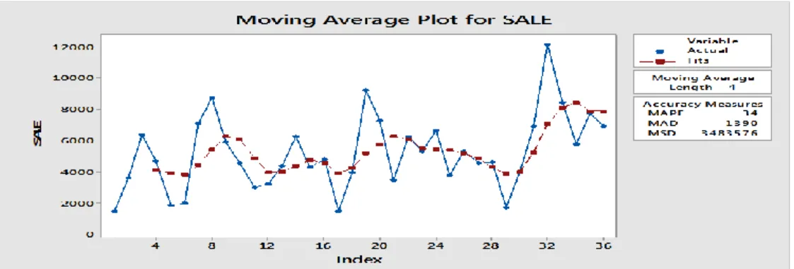
In double exponential smoothing method, nine trials were taken and different values of αand βare put in the equation (3). Least value of mean square deviation (MSD) is obtained at α =0.1,β=0.1as given in Table 3.
Table 3. Different Values of MSD for Double Exponential
Double exponential
α=0.1 α=0.1 α=0.1 α=0.2 α=0.2 α=0.2 α=0.3 α=0.3 α=0.3
β=0.1 β=0.2 β=0.3 β=0.1 β=0.2 β=0.3 β=0.1 β=0.2 β=0.3
Figure 4. Double Exponential Smoothing Plot for Sale
In Winter method, initial values of the smoothed series Lt, trend Tt, and the seasonality
indices It are put in equation (4). There are two types of models namely Multiplicative and Additive. The multiplicative model is used when the magnitude of the seasonal pattern increases as the series goes up and decreases as the series goes down and the additive model is used when the magnitude of the seasonal pattern does not change as the series goes up or down. In this work, additive model has been used because the magnitude of the seasonal pattern in our data does not change as the series goes up or down.Here, 27 different trials have been conductedby considering three cases. In the first case α =0.1 & β and γ ranging from 0.1 to 0.3 makes nine runs. Similarly α =0.2 and 0.3 are taken for different value of β and γ ranging from 0.1 to 0.3 makes 9 runs each in second and third case respectively, seasonal length is taken as 12. Least MSD value is calculated for each case as given in Table 4.The accuracy of winter’s method strongly depends on theoptimal values of alpha (α), beta (β), and gamma (γ). The optimal α, β and γ were determined byminimizing a measure of forecast error of MSD.
Table 4. Least Value of MSD for Winters Method
Winter’s method α=0.1 α=0.2 α=0.3
β & γ=0.1 to 0.3 β & γ=0.1 to 0.3 β & γ=0.1 to 0.3 Number of
experiments
9 9 9
Best combination α=0.1,β=0.1,γ=0.1 α=0.2,β=0.1,γ=0.1 α=0.3,β=0.1,γ=0.1
MSD 1697198 1730476 1795574
Figure 5. Winter’s Method Plot for Sale
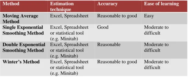
In the present work, different forecasting models for sale of a boot in shoe industry have been discussed. Method estimation techniques of these models are shown in Table 5.
Table 5. Check List for Selecting Appropriate Method
Method Estimation technique
Accuracy Ease of learning
Moving Average Method
Excel, Spreadsheet Reasonable to good Easy Single Exponential Smoothing Method Excel, Spreadsheet or statistical tool (e.g. Minitab) Good Moderate to difficult Double Exponential Smoothing Method Excel, Spreadsheet or statistical tool (e.g. Minitab) Reasonable Moderate to difficult
Winter’s Method Excel, Spreadsheet
or statistical tool (e.g. Minitab)
Reasonable to good Moderate to difficult
6. Conclusion
In this work, various types of forecasting methods are used for the determination of future sale of the product. The forecasting method will be selected on the basis of forecast error. Lesser the forecast error, the more accurate forecasting method.The specific purpose of this study was to identify the best quantitative forecasting method, based on level of accuracy and the ease of use in practice, to forecast demand of the Boot for Shoe Industry.
This study identified that many real-life forecasting situations were more complicated and difficult due to such variables as weather and special festival. Therefore, Tej International should applied appropriate quantitative methods to obtain better forecasting accuracy and to establish their strategic production plan of Boot product. Such forecasts can provide valuable information for production, facility monitoring, seasonal employment, short-term and long-term budgeting.
References
[1] R. T. Peterson, “Forecasting practices in the retail industry”, Journal of Business Forecasting, vol. 12, (1993), pp. 11-14.
[2] H. K. Alfares and M. Nazeeruddin, “Electric load forecasting: literature survey and classification of methods”, International Journal of Systems Science, vol. 33, no. 1, (2002), pp. 23-34.
[3] W. Peter and S. Anders, “Evaluation of forecasting error measurements and techniques for intermittent demand”, International journal of production economics, vol. 128, (2010), pp. 625-636.
[4] C. Cacatto, P. Belfiore and J. G. V. Vieira, “Forecasting practices in Brazilian food industry”, Journal of logistics management, vol. 1, no. 4, (2012), pp. 24-36.
[5] M. Sanwlani and M. Vijayalakshmi, “Forecasting sales through time series clustering”, International journal of data mining & knowledge management process, vol. 3, no. 1, (2013), pp. 39-56.
[6] D. P. Patil, A. P. Shrotri and A. R. Dandekar, “Management of uncertainty in supply chain”, International Journal of Emerging Technology and Advanced Engineering, vol. 2, no. 5, (2013), pp. 303-308.
[7] A. K. Sharma, A. Gupta and U. Sharma, “Electricity forecasting of Jammu & Kashmir: A methodology comparison”, International Journal of Electrical Engineering & Technology, vol. 4, no. 2, (2013), pp. 416-426.
[8] C. D. Ezeliora, “Moving average analysis of plastic production yield in a manufacturing industry”, International journal of multidisciplinary sciences and engineering, vol. 4, no. 2, (2013), pp. 65-73.
[9] K. Ryu and A. Sanchez, “The evaluation of forecasting methods at an institutional foodservice dining facility”, The Journal of Hospitality Financial Management, vol. 11, no. 1, (2003), pp. 27-45.
[10] E. Leve'n and A. Segerstedt, “Inventory control with a modified Croston procedure and Erlang distribution”, International Journal of Production Economics, vol. 90, (2004), pp. 361-367.
[11] A. A. Syntetos and J. E. Boylan, “The accuracy of intermittent demand estimates”, International Journal of Forecasting, vol. 21, (2005), pp. 303-314.
[12] A. A. Syntetos and J. E. Boylan, “On the bias of intermittent demand estimates”, International Journal of Production Economics, vol. 71, (2001), pp. 457-466.
[13] J. J. Strasheim, “Demand forecasting for motor vehicle spare parts”, A Journal of Industrial Engineering, vol. 6, no. 2, (1992), pp. 18-19.
[14] C. Floros, “Forecasting the UK unemployment rate: model comparisons”, International Journal of Applied Econometrics and Quantitative Studies, vol. 2, no. 4, (2005), pp. 57-72.
[15] S. Chopra and P. Meindl, “Supply Chain Management Strategy, Planning and Operation”, Pearson, 4th Ed, India, (2010).
[16] P. Y. Lim and C. V. Nayar, “Solar irradiance and load demand forecasting based on single exponential smoothing method”, International Journal of Engineering and Technology, vol. 4, no. 4, (2012), pp. 451-455.
[17] J. S. Armstrong and F. Collopy, “Error measures for generalizing about forecasting methods: Empirical comparisons”, International Journal of Forecasting, vol. 8, no. 1, (1992), pp. 69-80.