Explaining non-performing loans in Greece: a comparative study on the effects of recession and banking practices

Explaining Non-Performing Loans in

Greece: A Comparative Study on the

Effects of Recession and Banking Practices

Platon Monokroussos, Dimitrios D. Thomakos,

Thomas A. Alexopoulos

GreeSE Paper No.101

Hellenic Observatory Papers on Greece and Southeast Europe

TABLE OF CONTENTS

ABSTRACT ___________________________________________________________ 2 1. Introduction _____________________________________________________ 4 2. Determinants of non-performing loans: literature review and testable

hypotheses __________________________________________________________ 9 2.1 Macroeconomic determinants of credit risk _________________________ 12 2.2 Bank-specific determinants of credit risk ____________________________ 13 2.3 Feedback from NPLs to the real economy ___________________________ 16 3. Evolution of problem loans in Greece ________________________________ 16 4. Data and variables _______________________________________________ 20 4.1 Data _________________________________________________________ 20 4.2 Variables _____________________________________________________ 20 4.3 Methodology __________________________________________________ 23 5. Empirical analysis and policy implications ____________________________ 27 5.1 VEC representation _____________________________________________ 27 5.2 VAR representation _____________________________________________ 34 5.2.1 NPL VARs with macro determinants ______________________________ 36 5.2.3 Are the effects of macroeconomic shocks uniform across different NPL categories? _______________________________________________________ 51 5.2.4 NPL VARs for restructured loans _________________________________ 52 6. Concluding remarks and policy implications ___________________________ 53 References _________________________________________________________ 55

Explaining Non-Performing Loans in

Greece: A Comparative Study on the

Effects of Recession and Banking Practices

Platon Monokroussos

*

, Dimitrios D. Thomakos

#

,

and Thomas A. Alexopoulos

ⱡ

ABSTRACT

Using a new dataset of macroeconomic and banking-related variables we attempt to explain the evolution of “bad” loans in Greece over the period 2005-2015. Our findings suggest that the primary cause of the sharp increase in non-performing loans (NPLs) following the outbreak of the sovereign debt crisis can be mainly attributed to the unprecedented contraction of domestic economic activity and the subsequent rise in unemployment. Furthermore, our results offer no empirical evidence in support of a range of examined hypotheses assuming overly aggressive lending practices by major Greek credit institutions or any systematic efforts to boost current earnings by extending credit to lower credit quality clients. We find that the transmission of macroeconomic shocks to NPLs takes place relatively fast, with the estimated magnitude of the respective responses being broadly comparable with that documented in some earlier studies for other euro area periphery economies. Overall, our results support a swift implementation of reforms agreed with official lenders in the context of the new (3rd) bailout programme. These envisage the modernization the county’s private sector insolvency framework and the creation of a more efficient model for the management of NPLs. A vigorous implementation of these reforms is key for allowing a resumption of positive credit creation, by freeing up valuable resources that are currently trapped in unproductive sectors of the domestic economy. This, in turn, would facilitate a speedier return to positive economic growth and a gradual reduction in unemployment.

―――――――――――――――

*Dr. Platon Monokroussos, Group Chief Economist of Eurobank Ergasias S.A., LSE Hellenic Observatory Visiting Senior Fellow

#Dimitrios D. Thomakos, Professor in Applied Econometrics, University of Peloponnese ⱡThomas A. Alexopoulos, Ph.D. Candidate, University of Peloponnese

Explaining Non-Performing Loans in

Greece: A Comparative Study on the

Effects of Recession and Banking Practices

1.

Introduction

Exploring the determinants of non-performing loans (NPLs) is an issue of great importance for macroeconomic and financial-system stability. A large number of recent studies examine the drivers of credit risk, especially in the period after the outbreak of the global financial crisis. Some contributions in this field use a single category of potential determinants, while others focus on both systematic factors (e.g. general macroeconomic conditions) and idiosyncratic influences (e.g. bank-specific variables and firm-level information).

Our study utilizes a novel set of macroeconomic and microeconomic variables to explain the evolution of bad loans in the Greek banking system over the period 2005-2015. The models presented provide a suitable framework for analyzing banking sector developments in Greece and, by extension, in other euro area economies that were particularly hit by the sovereign debt crisis. Apart from being useful for empirically testing a number of relevant hypotheses, they allow the analysis of potential feedback effects from ex-post credit risk to the real economy. By and large, we believe that our findings constitute an important contribution to the literature. First, Greece has been particularly hit by the crisis, with draconian fiscal austerity measures being implemented in

recent years to address severe macroeconomic imbalances accumulated following the adoption of the euro. In the context of three consecutive bailout programmes implemented since mid-2010, a range of conventional and unconventional policies has been applied to stabilize the country’s economy and fiscal accounts. Arguably, these policies have had important consequences for private sector solvency and, by implication, for financial system stability.1,2 Therefore, it does not come as a surprise that Greece’s current bailout programme features domestic financial stability as one of its main pillars, with particular emphasis being placed on the management of NPLs and reforms to the domestic regulatory and legal framework in dealing with private sector insolvency. In view of the above, we believe that a thorough understanding of the determinants of credit risk is of utmost importance for designing appropriate policies aiming to safeguard macroeconomic and financial systemic stability in Greece and in other euro area periphery economies in the post-crisis era.

Second, our study features a number of novel aspects compared to a few relevant contributions for Greece that appeared in the literature in recent years (see e.g. Louzis et al., 2012; Makri et al., 2014; and Makri, 2015). In more detail, it utilizes a fully-updated set of macroeconomic and banking-sector quarterly data spanning the period 2005-2015. This

1 _{Over the period 2009-2015, Greece suffered cumulative GDP losses in excess of 25 percentage}

points (ppts), while the unemployment rate has increased by more than 17ppts. In addition, the unprecedented (in size and scope) restructuring of privately-held Greek pubic debt (PSI) in early 2012 completely wiped out the capital base of Greek banks, necessitating a major recapitalization of the domestic banking system in the following year. Two additional recapitalizations of systemic Greek banks followed (in 2014 and 2015) to address severe liquidity and solvency problems faced by these

time-horizon covers a significant part of the high growth period that followed the country’s euro area entry as well as the years after the outbreak of the Greek sovereign debt crisis in late 2009/early 2010. In more detail, we examine the evolution of realized credit risk by looking at a supervisory set of quarterly data for aggregate (banking system-wide) non-performing loans3 as well as the respective data for consumer, mortgage and corporate loans. In contrast to earlier studies for Greece, which mostly analyze problem loans excluding restructurings, we also look at the determinants of non-performing loans that include restructured loans.4 This has been possible by working with an entirely new set of data compiled by the Bank of Greece and constitutes a quite interesting aspect of our study, as it allows us to also look at the evolution of restructured loans.

Third, compared to the data panel estimation methods that have been mostly used in earlier studies, we estimate a number of vector error correction (VEC) and vector autoregession (VAR) models. This gives us the additional advantage of addressing potential endogeneity issues. Furthermore, it allows us to fully capture the dynamic interactions between different types of bad loan determinants and examine the feedback of NPLs to other variables, both macroeconomic and banking-sector specific ones.

3

In our analysis, non-performing loans are defined as bank loans overdue by more than ninety (90) days.

4

A significant portion of problem loans have been restructured in Greece over the last several years, following direct borrower-creditor negotiations to modify their terms. At the end of 2015, the outstanding amount of problem loans in domestic banks’ balance sheets stood at c. €98.4bn (or 43.5 percent of total outstanding loans), while the respective level which excludes restructured loans was c. €80.5bn (or 35.6 percent of total loans). So far, loan restructuring has mostly taken the form of maturity extensions.

In addition to examining the robustness of some earlier empirical findings in the context of our extended data set, we test a number of new hypotheses that appear to have important policy implications. Among others, we empirically document that the primary cause of the sharp increase of non-performing loans in Greece following the outbreak of the sovereign debt crisis can be mainly attributed to the unprecedented contraction of domestic economic activity (and the subsequent spike in unemployment) and not to the high rates of domestic credit expansion experienced in the initial period following the euro adoption. In fact, our findings offer no empirical evidence in support of a range of examined hypotheses assuming overly aggressive lending practices by major Greek banks or any systematic efforts to boost current earnings by extending credit to lower credit quality clients. Furthermore, the transmission of macroeconomic shocks to NPLs takes place relatively fast, with the estimated magnitude of the respective responses being broadly comparable with that documented in the earlier literature. For instance, in a bivariate VAR model for the quarterly change in the ratio of NPLs (including restructured loans) and real GDP growth, the maximum impact of a GDP shock is felt within 3 quarters, while the magnitude of the estimated long-term impact is a c. 0.4 percentage points (ppts) increase in the NPLs ratio per 1 ppt contraction in real GDP growth.

In most estimated models we document a significant feedback effect running from NPLs to real GDP growth and the unemployment rate. In other words, an increase in the NPLs ratio can have a measurable (and

and employment conditions. Such a two-way causality between bad loans and the macro economy has been documented in a number of earlier studies (for instance, see Diawan and Rodrik, 1992) and it can materialize through e.g. the credit supply channel. In more detail, a high volume of bad loans typically implies increased operating costs for their monitoring and management as well as higher provisioning, a situation that hinders capital adequacy and financing terms for credit institutions. These factors may in turn lead to higher lending interest rates and, more generally, tighter lending conditions in the economy. Finally, in line with some recent empirical studies for Greece (see e.g. Louzis et al., 2012), we find that the magnitude (and the significance) of the impact of macroeconomic conditions on the evolution of NPLs can vary across different categories of loans (consumer, mortgage or corporate).

Overall, our results urge for a swift stabilization of domestic economic conditions that would allow a cyclical peak in the non-performing loans ratio not far from its current (end-2015) level. The rigorous implementation of the conditionality underlying the new (3rd) bailout programme agreed with official lenders in August 2015 constitutes an important prerequisite for attaining this aim. In this context, the implementation of agreed reforms for modernizing the county’s private sector insolvency framework and for moving towards a more efficient model for the management of NPLs is key for allowing a resumption of positive credit creation, by freeing up valuable resources that are currently trapped in unproductive sectors of the Greek economy.

The rest of this paper is structured as follows: section 2 provides a literature review of the macro- and micro-related determinants of NPLs; section 3 provides a bird’s eye view on the evolution of problem loans in Greece in the years before and after the outbreak of the global crisis; section 4 discusses our data and empirical methodology; section 5 presents our empirical results and their policy implications; and section 6 offers some concluding remarks.

2.

Determinants of non-performing loans: literature review and

testable hypotheses

Many studies on the causes of bank failures have documented that failing institutions usually feature a higher volume of problem loans prior to failure and that asset quality constitutes a statistically significant predictor of insolvency (Berger and DeYoung, 1997). The literature on the determinants of credit risk identifies several important categories of potential determinants, ranging from macroeconomic and institutional factors to bank-specific variables and firm-level information.

Models examining the influence of macroeconomic factors on credit risk focus primarily on the relationship between the business cycle and the capacity of borrowers to service their loans. The central idea underlying these studies is that credit standards undergo a gradual deterioration during economic expansion, when credit institutions apply increasingly liberal lending policies in their quest for market share (see e.g. Keeton, 1999 and Fernandez De Lis et al., 2000). These may take the form of

increased lending to low credit quality borrowers (Rajan, 1994). Such strategies usually backfire during recessionary phases, when credit risks actually materialize. Recent studies examining the role of the business cycle in the evolution of credit risk include e.g. Borio et al. (2001), Quagliarello (2007), Beck et al. (2013) and Climent-Serrano and Pavia (2014).

Studies examining the impact of lending strategies use bank-specific information as explanatory variables in models analyzing the inter-temporal evolution of bad loans and/or other measures of ex-post credit risk. Such information relates to, among others, loan quality, cost efficiency and capitalization of credit institutions, with a number of relevant hypotheses having been examined in the literature, starting with the seminal work of Berger and DeYoung (1997).

Another strand of the literature looks at firm-specific information to account for the idiosyncratic components of credit risk. Relevant studies focus on a number of accounting variables as potential determinants of bad loans and/or other proxies for corporate credit risk. These include e.g. firm sales growth, profitability, funding cost, leverage, asset growth, size and age. Contributions belonging to this group of studies include e.g. Benito and Young (2001); Bunn and Redwood (2003) and Belaid (2014).

Separately, a group of studies looks at the potential impact of the business and regulatory environment on the level of banks’ problem loans. Such studies examine the significance of various indicators of the

quality and the stability of a country’s legal, regulatory, institutional and political environment. Among others, relevant measures may include the degree of information sharing between creditors and borrowers, the legal rights of borrowers and lenders (as reflected in e.g. the presence or not of a sound bankruptcy framework) as well as the degree of corruption control. Studies examining the impact of such regulatory and institutional factors include e.g. La Porta, et al. (1998); Galindo and Miller (2001); Jappelli and Pagano (2002); Godlewski (2004) and Djankov et al. (2007).

More recently, an increasing number of studies estimate models that combine the aforementioned categories of variables in explaining the evolution of credit risk. For instance, Quagliarello (2006) combines macroeconomic and bank-specific determinants to investigate the riskiness (as proxied by the evolution of loan loss provisions and the flow of new bad loans ratio) of a large database of Italian intermediaries over the period 1985-2002. In a similar vein, Louzis et al. (2012) use a balanced panel consisting of supervisory data for the nine largest Greek commercial banks to test a number of hypotheses and explain the intertemporal evolution of the non-performing loans in Greece over the period from Q1 2003 to Q3 2009. Bonfim (2009) uses macroeconomic variables and firm-specific information to explain the determinants of credit default in the Portuguese banking industry. Separately, Belaid (2014) combines macroeconomic and bank-specific variables with a data set containing information for more than nine thousand domestic firms to explain the loan quality determinants in the Tunisian banking sector

Finally, Boudriga et al. (2010) analyze empirically the determinants of non-performing loans and the potential impact of both the business and the institutional environment on credit risk exposure of banks in the MENA region. By looking at a sample of 46 banks in 12 countries over the period 2002-2006 they find that credit quality of banks is positively affected by the relevance and the quality of credit information published by public and private bureaus. Their findings also highlight the importance of a sound institutional environment in enhancing bank credit quality. According to their analysis, a better control of corruption, sound regulatory quality, a better enforcement of the rule of law, and free voice and accountability play an important role in reducing NPLs in the MENA countries.

For the purpose of our empirical analysis, we elaborate below on the first two general categories of potential credit risk determinants; namely, macroeconomic factors and bank-specific variables.

2.1 Macroeconomic determinants of credit risk

The empirical literature examining the link between credit risk and the state of the macro economy dates back to the papers of King and Plosser (1984), Bernanke and Gertler (1989), and Bernanke, Gertler and Gilchrist (1998). These along with a number of more recent studies generally document a negative relationship between macroeconomic conditions and non-performing loans (NPLs). A general explanation for this finding is as follows: in economic expansions borrowers’ income improves and thus, their capacity to service their debts. On the other hand, when economic activity slows down, NPLs increase as unemployment rises, disposable incomes decline and borrowers face difficulties in repaying

their debt obligations (Salas and Suarina, 2002; Rajan and Dhal 2003; Jimenez and Saurina, 2005; Pesaran et al., 2006; Quagliarello 2007; Beck et al., 2013; and Klein 2013).

Other macroeconomic variables that potentially affect the debt servicing capacity of firms and households and, by implication, banks’ asset quality include the unemployment rate, inflation, property prices as well as the loan interest rate and the exchange rate. In more detail, many empirical studies document a positive link between lending interest rates and NPLs, particularly in the case of floating rate loans (see e.g. Louzis et al., 2012; Beck et al., 2013 and Klein 2013). However, the impact of inflation on asset quality may be ambiguous. Higher inflation erodes the real value of outstanding debt, thus making debt servicing easier. On the other hand, it may reduce real incomes (when prices are sticky) and/or instigate an interest rate tightening by the monetary authority (Nkusu, 2011). Finally, several studies find a negative link between share prices and NPLs, as a pronounced decline in the stock market may reflect an expected deterioration in broader macroeconomic conditions, a high number of corporate defaults and an erosion of collateral values (see e.g. Beck et al., 2013).

2.2 Bank-specific determinants of credit risk

The lending policies of credit institutions play a central role in the evolution of future problem loans. In line with the stylized fact of credit pro-cyclicality5, the market share conquest campaigns undertaken by credit institutions in conjunction with the income smoothing activities by

borrowers in expansionary phases may give rise to inadequate credit quality assessments or even worse to “gambling resurrection” policies on the part of bank managers (see e.g. Fernandez et al., 2000).6

This situation usually leads to an acceleration of banks’ lending activities during periods of positive economic growth, which are often accompanied by a gradual loosening of credit standards, especially in the more mature stages of the economic upturn. However, the implications of worsened credit standards for macroeconomic and financial-system stability do not become fully apparent before a new major economic downturn materializes.

In an economic recession, the rise of unemployment and the decline in household and corporate incomes hinder the debt servicing ability of borrowers. To exacerbate things further, the incipient rise in problem loans and the decline in collateral values lead to a serious tightening of credit conditions as banks become increasingly unwilling to extend new credit in an environment characterized by increased information asymmetries with respect to the actual credit quality of borrowers. The whole situation then gives rise to boom-bust credit cycles that move in synch with the economy’s up and down phases or even worse to major banking sector crisis as analyzed in e.g. Pesola (2005).

In their influential study, Berger and DeYoung (1997) look at the effect of banks’ lending strategies and other activities on asset quality. In more

6 _{In this context, “gambling resurrection” policies can be thought as highly speculative lending}

detail, they examine the relationship between NPLs, cost efficiency and capitalization of U.S. commercial banks over the period 1985-94 by testing a number of hypotheses concerning the direction of causality among these variables. They find a negative link (and a two-way causality) between cost efficiency and NPLs as: (i) an exogenous increase in non-performing loans - driven by, say, a notable worsening in the broader macroeconomic conditions - may lead to a deterioration in banks’ cost efficiency as a result of increased operating costs to deal with NPLs (“bad luck” hypothesis); and (ii) low cost efficiency may signify poor management skills in credit scoring as well as in loan underwriting monitoring and control, which, in turn, can lead to higher NPLs (“bad management” hypothesis).

An alternative hypothesis (dubbed as “skimping”) advanced by Berger and DeYoung (1997), proposes a positive relationship between cost efficiency and NPLs. This is on the basis that high cost efficiency may reflect limited resources allocated to monitor credit risk, a situation that could lead to higher problem loans in the future. Finally, Berger and DeYoung (1997) as well as a number of later studies examine the so-called “moral hazard” hypothesis, initially proposed by Keeton and Morris (1987). The latter hypothesis claims that low capitalization of banks leads to higher NPLs as banks’ managers may have an incentive to carry riskier loan portfolios. In line with these empirical findings, a number of recent studies find support of some of the aforementioned hypotheses.

2.3 Feedback from NPLs to the real economy

In a number of empirical studies, the feedback from NPLs to the real economy is usually identified through the credit supply channel. For instance, a high volume of bad loans typically implies increased operating costs for their monitoring and management as well as higher provisioning, a situation that hinders capital adequacy and financing terms for credit institutions. These factors may in turn lead to higher lending interest rates and, more generally, tighter lending conditions in the economy (Diawan and Rodrik, 1992). The feedback effects from NPLs to the real economy may also work through non-credit supply channels, as, for instance, debt overhang can discourage companies from investing in new projects since future profits will be shared with the creditors (Myers, 1977).

3.

Evolution of problem loans in Greece

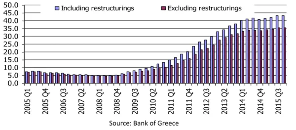
In Greece, a country that has experienced one of the most severe and prolonged recessions in recent economic history, cumulative real GDP losses between Q1 2008 and Q4 2015 amounted to around 26 percent, while the ratio of non-performing loans to total loans increased by 30.9ppts (and by 38.4ppts if restructured loans are also accounted for), hitting 35.6 percent (and 43.5 percent, respectively) at the end of that period (Figure A). This followed double-digit growth of domestic bank lending in the post euro-entry years that led to the 2007/2008 global financial crisis (Figure B). However, it is important to note that the global crisis found Greece’s private sector not particularly over-levered relative

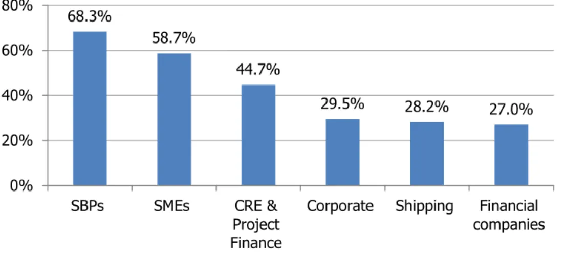
to other euro area economies (Figure C). In terms of nominal amounts, the total outstanding stock of NPLs (including restructured loans) in Greek commercial banks’ balance sheets stood at €98.4bn at the end of 2015, with corporate bad loans accounting for 57.1 percent of the total stock (Figure D). The overwhelming portion of the latter share consists of bad debts owed by very small, small and medium-sized firms (Figure E). The corresponding percentages for mortgage and consumer problem loans were 27.6 and 15.2 at the end of 2015. In terms of provisioning, the coverage of NPLs including restructured loans by loan loss reserves ranged between 45 and 55 percent during the initial part of our sample (Q1 2005 – Q4 2008). The said coverage fell precipitously in the following few quarters (hit a low of 31.8 percent in Q4 2009), before increasing gradually thereafter and hitting a post-crisis high of 46.4 at the end of 2015 (Figure F). Finally, a look at Figure G indicates that the flow (here, the quarterly change of the level) of NPLs including restructured loans embarked on an upward path after the outbreak of the global crisis, hitting a record peak of €13.8bn in Q1 2013. This compares with an average quarterly flow of c. €3.5bn in the prior three years and can be mainly attributed to the absorption of the balance sheets of the Cypriot subsidiaries in Greece by the four Greek systemic banks. The pace of increase of the said flow measure declined significantly in 2014 (it even recorded a negative reading of c. - €2.4bn in Q4 2014), it hit a two-year high in Q1 2015 (€2.35bn) and ended that year with a small increase of €0.2bn.

Figure A - Greek commercial banks' non-performing loans (with and without restructured loans) to total loans ratio in percentage points

0.0 5.0 10.0 15.0 20.0 25.0 30.0 35.0 40.0 45.0 50.0 20 05 Q 1 20 05 Q 4 20 06 Q 3 20 07 Q 2 20 08 Q 1 20 08 Q 4 20 09 Q 3 20 10 Q 2 20 11 Q 1 20 11 Q 4 20 12 Q 3 20 13 Q 2 20 14 Q 1 20 14 Q 4 20 15 Q 3

Including restructurings Excluding restructurings

Source: Bank of Greece

Figure B – Annual growth of the outstanding balances of Greek commercial bank loans (before provisions) & non-performing loans including restructured loans in percentage points

-20.0% -10.0% 0.0% 10.0% 20.0% 30.0% 40.0% 50.0% 60.0% 70.0% 80.0% 2002 2003 2004 2005 2006 2007 2008 2009 2010 2011 2012 2013 2014 2015

Bank loans (YoY, %) NPLs (YoY, %)

Source: Bank of Greece

Figure C – Private sector credit to GDP (end-2008)

0.0 50.0 100.0 150.0 200.0 250.0 300.0 Slov aki a R oman ia Cz ec h Re p. Pola nd US Hu ng ary Li th uani a B elg iu m B ulga ria Ca nada Finla nd It aly Slov eni a La tvi a Ge rmany Fran ce A us tri a Es ton ia Lux em bour g Ja pa n _UK Gre ec e N et he rla nd s Sw ed en M alt a A us tral ia N ew Ze ala nd Port uga l Sp ai n Ire la nd Denm ark Cy pru s AVERAGE = 102.4

Figure D – Evolution of non-performing loans including restructured loans by major sectors in Greece (EUR billions)

0.00 20.00 40.00 60.00 80.00 100.00 120.00 20 05 Q 1 20 05 Q 4 20 06 Q 3 20 07 Q 2 20 08 Q 1 20 08 Q 4 20 09 Q 3 20 10 Q 2 20 11 Q 1 20 11 Q 4 20 12 Q 3 20 13 Q 2 20 14 Q 1 20 14 Q 4 20 15 Q 3 Corporate Mortgage Consumer

Source: Bank of Greece

Figure E – Non-performing corporate exposures to total corporate loans ratio at the end of 2015 (percentage points) 68.3% 58.7% 44.7% 29.5% _{28.2% 27.0%} 0% 20% 40% 60% 80%

SBPs SMEs CRE &

Project Finance

Corporate Shipping Financial companies Source: Bank of Greece

Figure F – Non-performing loans including restructured loans to total loans ratio; loan loss reserves to total loans ratio and coverage of non-performing loans (percentage points)

0.0 10.0 20.0 30.0 40.0 50.0 05 Q 1 05 Q 4 06 Q 3 07 Q 2 08 Q 1 08 Q 4 09 Q 3 10 Q 2 11 Q 1 11 Q 4 12 Q 3 13 Q 2 14 Q 1 14 Q 4 15 Q 3 20.0 30.0 40.0 50.0 60.0 NPL to total loans ratio (lhs)

LLR to total loans ratio (lhs)

Figure G– Quarterly change (flow) of the total outstanding amount of loans classified as bad debt including restructured loans (EUR billions)

-4.0 0.0 4.0 8.0 12.0 16.0 2 0 0 5 Q 1 2 0 0 5 Q 3 2 0 0 6 Q 1 2 0 0 6 Q 3 2 0 0 7 Q 1 2 0 0 7 Q 3 2 0 0 8 Q 1 2 0 0 8 Q 3 2 0 0 9 Q 1 2 0 0 9 Q 3 2 0 1 0 Q 1 2 0 1 0 Q 3 2 0 1 1 Q 1 2 0 1 1 Q 3 2 0 1 2 Q 1 2 0 1 2 Q 3 2 0 1 3 Q 1 2 0 1 3 Q 3 2 0 1 4 Q 1 2 0 1 4 Q 3 2 0 1 5 Q 1 2 0 1 5 Q 3

Source: Bank of Greece

4.

Data and variables

4.1 Data

For the purpose of our empirical analysis, we utilize a novel data set of macroeconomic and bank-specific variables (quarterly observations) spanning the period between Q1 2005 and Q4 2015. Our data sources include Bank of Greece, Greece’s statistics agency (EL.STAT.) and EUROSTAT.

4.2 Variables

Depending on the model specification under examination, the variables presented below are expressed in log levels, ratios or percentages in the case of interest rates.

Realized credit risk variables

Many banking variables are potentially able to convey signals about the evolution of banks’ riskiness over the business cycle; however, loan loss provisions and non-performing loans have generally been considered to

be the main transmission channels of macroeconomic shocks to banks’ balance sheets (Quagliarello, 2007). For the purpose of our analysis, we estimate alternative models featuring the following credit risk variables:

Non-performing loans: bank loans overdue for more than ninety (90)

days. For the purposes of our analysis, we utilize supervisory data for the aggregate (industry-wide) stock of bad loans as well as the corresponding series for consumer, mortgage and corporate loans. The respective acronyms we assign to these variables are: TNPL (total stock of bad loans); TNPL_CONS (consumer bad loans), TNPL_HOUSE

(mortgage bad loans); and TNPL_CORP (corporate bad loans).

Restructured loans ratio: total stock of restructured loans (all types of

loans) with the respective acronym being: L_RESTRUCT.

The rest of the variables in our study belong to two broad categories of potential explanatory variables of credit risk that have been identified in the literature; namely: macroeconomic variables and bank-specific variables.

Macroeconomic variables

Real GDP (RGDP): an aggregate indicator of the state of the macro

economy and the phase of the business cycle. As explained earlier, we would expect a negative relationship between this variable and the ratio of bad loans to total loans.

Labour market conditions: two alternative indicators of labour market

conditions are examined in the study; namely, unemployment rate as a percentage of the total labour force (UNPL) and the total number of

earlier, we would expect a negative relationship between labour market conditions and the ratio of bad loans to total loans (positive association if the unemployment rate in levels or first differences is used).

Domestic inflation (INFL): herein proxied by the quarterly change in the

harmonized consumer price index for Greece. As explained earlier, the impact of inflation on future bad debts may be ambiguous.

Collateral values: index of prices of dwellings, deflated by the

harmonized inflation rate for Greece (RHP).7 Based on the analysis above, we would expect a negative relationship between collateral values and NPLs.

Debt service cost: real interest rate on bank loans calculated using as

weights the outstanding volumes of domestic monetary financial institutions’ loans vis-à-vis euro area private-sector residents (L_RIR); the respective acronyms for the real interest rate on consumer, mortgage and corporate loans are: L_CONS_RIR, L_HOUSE_RIR and

L_CORP_RIR.

Bank-specific variables:

Loans-to-deposits interest rate spread (LD_IRS): this variable may be

given alternative interpretations e.g. relative competitiveness conditions in the loans and deposits market or degree of risk taking on the part of domestic credit institutions (positive association with NPLs).

Growth of the stock of performing loans: loans excluding NPLs and

restructured loans, with respective acronyms: PERFO_TL_GR (total aggregate stock); PERFO_CONS_GR (consumer); PERFO_HOUSE_GR

(mortgage); and PERFO_CORP_GR (corporate loans);

7 _{Bank of Greece publishes a newer index based on apartment prices. However, our study uses the}

Bank solvency and capitalization: industry-wide solvency ratio, measured as total common shareholders equity to total bank assets (ETA). In line with the literature, the finding of a negative relationship between bank solvency and future bad loans may be interpreted as empirical evidence supporting the so-called “moral hazard” hypothesis i.e., low capitalization of banks may lead to an increase in future NPLs as bank managers may have an incentive to carry riskier loan portfolios.

4.3 Methodology

This section outlines the methodology used in the study, which is mostly dictated by the nature of the available data. Since our time series are relatively short, we avoid complicated methods that would potentially require a larger data sample. We therefore employ an unrestricted vector autoregression (VAR) in levels and in differences as well as a vector error correction (VEC) model, with the aim to examine the robustness of the empirical results and the consistency of the policy implications that they imply. In this context, it is important to note that our VAR and VEC models are estimated using different underlying data (e.g. NPL ratios vs NPLs in levels, respectively), arguably enhancing robustness and protecting our analysis from (potentially severe) misspecifications.

The standard VAR model with p lags, when the variables are expressed in differences, is written as:

, , , , 1 p q k t i q k t i t t

y

A y

X

u





_ 



 





  

₍₁₎

matrices, utis i i d N. . (0, ) and Xt is an exogenous pseudo-variable, herein

the crisis dummy C12 as explained in the next section. The three subscripts in the vector of our variables are used to help identify the different models and variable combinations as follows.



. , , , , , , , [ , , , , _ , , _ , _ } ] , 1,..., 5 , 0 , 1 , _ & _ , 2 , 3 q k t k t t t t k t t t k t q k t k t k t

y TNPL UNPL RGDP RHP L RIR ETA LD IRS PERFO RG for q

Total loans k Corporate Loans k

where TNPL PERFO RG L RIR for q Mortgages k Consumer Loans k       _  _  _    

When we consider a standard VAR with p lags, when the variables are expressed in levels, we simply re-write the model of equation (1) without the difference operator as:

, , 1 ( 1) 1 p q k t i t i p t p t t i

y



A y

_

A

_

y

_{ }

X

u



 





  

₍₂₎

where we add an extra lag term which is required for accurately performing causality tests with non-stationary data (the discussion on causality testing follows after the presentation of the models). The corresponding VEC format of the VAR model is given in standard form as well: 1 , 1 1 p q t t i t i t t y y y X u         



     ₍₃₎

where yq t, is the following (Kx1) column vector:



, [ _ _ , _ , _ , _ _ , _ }]

q t t t t t t

y  LOG L TNPL LOG RGDP LOG EMPLOYED LOG L TLOANS L RIR 

and rk(Π)=r with 0<r<K so that  , where α and β are (K r )

pseudo-variables, herein the crisis dummies C12 and D2013 as explained in the next section. To test for the presence of co-integration we use the approach of Johansen (1991, 1995), using both the maximal eigenvalue and trace statistics. The error-correction term, ECT, is expressed in generic form as:

ECT



 

(



y

t1

 

c

0

d t

0

)

 

c

1

d t

1 ₍₄₎ Here we perform pre-testing for identifying where a constant and/or a linear term trend should be included in the error correction relationship. Depending on whether the co-integrating vector annihilates the trend component, we find that the parameters c0 and c1 should not simultaneously be included in our estimated specifications. The same applies for d0 and d1.

The optimal lag length is chosen by fitting the VAR representation of the models sequentially with lag orders p0,1,...,pmax and selecting the value that minimizes standard information criteria, with the following (generic) format:

~

( )

ln

u

( )

( , )

IC p





p



h p n

(5) where h(p,n) stands for the penalty function ~ 1

1 ˆ ˆ ( ) T u _{t t} t p T      



_{of the}

respective VAR(p) model. Depending on the penalty function that is being used, the information criteria are the Akaike Information criterion (AIC), the Schwarz criterion (SC) and the Hannan-Quinn criterion (HQ). We mostly rely on the latter for selecting the lag length.

Finally, we briefly illustrate below the causality testing, which is performed in a similar fashion for model specifications in both first differences and levels, with the only difference being the presence of the extra lag terms in equation (2). Partitioning the vector of interest in m-dimensional and (K−m)-m-dimensional sub-vectorsya t, andy,t:

, , a t t t y y y_        _and 11, 12, 21, 22, 1... i i i i i A A A i p A A   _{ }    ₍₆₎

where Ai are partitioned in accordance with the partitioning of yt,

,

a t

y does not Granger-cause y,tif and only if the following hypothesis

cannot be rejected:

H

o

:

A

12,i



0

for

i



1...

p

(7)

Thus, the null hypothesis is formulated as zero restrictions on the coefficients of the lags of a subset of the variables. This is in the form of a standard Wald-type test and therefore inference is asymptotically normal for both the VAR in differences in equation (1) and the lagged differences in the VEC model in equation (3). However, inference is non-standard when we consider the VAR in levels in equation (2) and therefore we adopt the methodology proposed by Toda and Yamamoto (1995), which restores asymptotically normal inference in causality testing and is robust to the integration and cointegration properties of the process. Therefore for equation (2), we apply Granger causality testing in the augmented dmax VAR(p) representation, where dmax is the maximum order of integration suspected to apply in the VAR.

Because our level variables are first order integrated we use an augmented (by one lag) VAR(p+1) as shown before.8

A set of standard residual and misspecification tests is applied after the estimation of each model, either in VAR or VEC form. Detailed results on these tests are available on request.

5.

Empirical analysis and policy implications

5.1 VEC representation

This section discusses the results of our co-integration analysis and the estimates of a number of identified error correction (VEC) models.9 The variables examined herein are taken in log levels and include:

LOG_L_TNPL: logarithm of the level of total (banking sector-wide)

non-performing loans that include restructured loans in billions of euros;

LOG_RGDP: logarithm of the level of Greece’s real gross domestic

product in billions of euros;

LOG_EMPLOYED: logarithm of the total number of employed individuals

in all domestic industries in millions of persons;

LOG_L_TLOANS: logarithm of the level of total outstanding loans

provided by domestic credit institutions in billions of euros; and

L_RIR: average weighted loan interest rate deflated by Greece’s

harmonized index of consumer prices, herein calculated using as weights

8

While we do not explicitly discuss impulse responses and variance decomposition in the methodology section we do note that the presence of causality is a prerequisite for their interpretability. This is the reason why we insist on examining the robustness of our causality tests across three different kinds of VAR representations, including levels, differences and VEC.

the outstanding volumes of domestic monetary financial institutions’ loans vis-à-vis euro area private-sector residents.

The results of our Augmented Dickey-Fuller and Phillips-Perron tests indicate that all of the aforementioned variables represent non-stationary I(1) processes.10 Furthermore, the implementation of VAR-based co-integration tests using the methodology developed in Johansen (1991, 1995) indicates the existence of one or more co-integrating relationships in different combinations of the variables under examination (results are available on request).

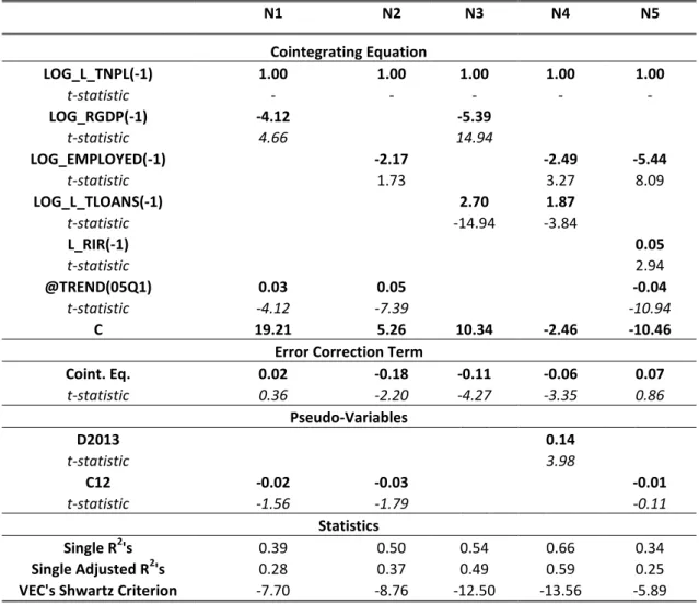
The estimates of our vector error correction (VEC) specifications are reported in Table 1.1 (models N1 to N5). The first part of the table (under the heading “Co-integrating Equations”) reports the results from the first step Johansen procedure and shows the long-run equilibrium relationship between the co-integrated variables of interest. Calculated t-statistics based on the estimated asymptotic standard errors (corrected for degrees of freedom) are reported below the estimated coefficients.

The rest of Table 1.1 has the usual interpretation. The lines under the heading “Error Correction Terms” show the estimated coefficient(s) of the error correction term(s) and effectively constitute speed of adjustment parameters. Similarly, the lines under the heading “Pseudo-Variables” show the coefficients of the dummy variables c12 and d2013.

10 _{Care must be taken in interpreting the results of such tests due to the limited sample size; unit root}

tests are not the best power performers. This is one of the reasons that we have opted to estimate more than one kind of models from the VAR family.

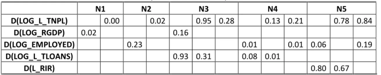
In our study, c12 is defined as a crisis dummy that takes the value 1 from Q1 2012 onwards and the value zero (0) otherwise, while d2013 takes the value 1 in Q1 2013 and the value zero in all other quarters. The latter dummy is meant to capture the effects of the one-off spike recorded in the level of non-performing loans in the first quarter of 2013 due to the absorption by the four Greek systemic banks of the balance sheets of the Cypriot subsidiaries operating in Greece following the outbreak of the Cypriot banking crisis. The usual goodness of fit measures R2 and Adjusted-R2 as well as the VEC Schwartz Criterion are reported below the heading “Statistics”, while Table 1.2 shows the results of the relevant Granger causality tests.

Table 1.1 Estimation results from Error Correction Models N1 to N5. (Source: The Authors)

N1 N2 N3 N4 N5 Cointegrating Equation LOG_L_TNPL(-1) 1.00 1.00 1.00 1.00 1.00 t-statistic - - - - - LOG_RGDP(-1) -4.12 -5.39 t-statistic 4.66 14.94 LOG_EMPLOYED(-1) -2.17 -2.49 -5.44 t-statistic 1.73 3.27 8.09 LOG_L_TLOANS(-1) 2.70 1.87 t-statistic -14.94 -3.84 L_RIR(-1) 0.05 t-statistic 2.94 @TREND(05Q1) 0.03 0.05 -0.04 t-statistic -4.12 -7.39 -10.94 C 19.21 5.26 10.34 -2.46 -10.46

Error Correction Term

Coint. Eq. 0.02 -0.18 -0.11 -0.06 0.07 t-statistic 0.36 -2.20 -4.27 -3.35 0.86 Pseudo-Variables D2013 0.14 t-statistic 3.98 C12 -0.02 -0.03 -0.01 t-statistic -1.56 -1.79 -0.11 Statistics Single R2's 0.39 0.50 0.54 0.66 0.34 Single Adjusted R2's 0.28 0.37 0.49 0.59 0.25

Table 1.2 P-values of the modified Wald-Test for causality for Error Correction Models N1 to N5. (Source: The Authors)

N1 N2 N3 N4 N5 D(LOG_L_TNPL) 0.00 0.02 0.95 0.28 0.13 0.21 0.78 0.84 D(LOG_RGDP) 0.02 0.16 D(LOG_EMPLOYED) 0.23 0.01 0.01 0.06 0.19 D(LOG_L_TLOANS) 0.93 0.31 0.08 0.01 D(L_RIR) 0.80 0.67

* All variables are in logs of levels

The first part of Table 1.1 indicates that all macroeconomic variables under examination have the correct theoretical sign and are statistically significant.

In more detail, the level of non-performing loans including restructured loans is negatively affected by (i.e., increases with) a slowdown in economic activity (models: N1 & N3) or a decline in the number of employed persons (models: N2, N4 & N5). This result confirms the importance of macroeconomic conditions for the evolution of bad debts and is in line with the findings of a number of recent empirical studies (see e.g. Salas and Suarina, 2002; Rajan and Dhal, 2003; Jimenez and Saurina, 2005; Pesaran et al., 2006; Quagliarello 2007; Beck et al., 2013; Klein 2013; and Louzis et al., 2012). Again, the general explanation for the countercyclical behavior of bad loans relates to the procyclicality of the demand and the supply of bank credit as well as the difficulties faced by borrowers in servicing their debt obligations when macroeconomic conditions deteriorate, unemployment rises and disposable incomes decline.

The estimated coefficient of the real interest rate in the estimated long-run equilibrium relationship of model N5 is statistically significant and

has the correct theoretical sign (positive). This finding is also in line with the earlier literature (see e.g. Louzis et al., 2012, Beck et al., 2013; and Klein 2013) and reflects the increased difficulty faced by borrowers in meeting their loan obligations when servicing costs increase.

The level of total loans enters the long-run equilibrium relationship with a positive (and significant) sign as regards its relationship with the level of non-performing loans (models N3 & N4). This is in line with what one should expect, given that an increase in the amount of loans provided by domestic banks increases the chances that a higher volume of loans will go bust when economic conditions deteriorate.

An interesting finding related to the estimates of model N3 is that the long-run effect (in absolute terms) of the level of real GDP on the level of non-performing loans is found to be around double in magnitude of the effect of loans provided by the domestic banking system. This is verified by testing the following restriction in the long-run co-integrating equation:

coefficientLOG_RGDP + 2* coefficientLOG_L_TLOANS = 0 (1)

The relevant Likelihood Ratio (LR) statistic for the testing of the above restriction is asymptotically distributed at chi-square with degrees of freedom equal to the number of cointegrating equation (herein, equal to 1). In our case, the estimated chi-square (1) value is 0.235 (probability: 0.628), which means that the imposed restriction cannot be rejected at usual confidence levels.

A potential interpretation of the above result is as follows: in Greece’s case, past experience suggests that aggregate economic activity (herein, proxied by real GDP) is much more important than the outstanding stock of bank credit in determining the level of non-performing loans in the long-run equilibrium. In turn, this highlights the importance of restoring the conditions for positive and sustainable economic growth for improving private-sector solvency. This result is also in agreement with the argument made in Sector 3 that the crisis found Greece’s private sector not particularly over levered relative to other euro area (and non-EA EU) economies, as least as regards the respective ratios of outstanding private-sector credit to GDP.

Taking model N1 to be our baseline specification, we document a bi-directional causality between the level of non-performing loans

(LOG_L_TNPL) and the level of real GDP (LOG_L_RGDP). In more detail,

as the Granger Causality tests of Table 1.2 indicates, TNPLs are Granger caused by RGDP at a 2.1% significance level, while RGDP is Granger caused by TNPLs at a significance level of 1%. Stating it differently, each variable is better explained by both the lagged values of TNPLs and RGDP than by its own lags alone. Reported results of Granger causality tests implemented in models N2 to N6 have an analogous interpretation.

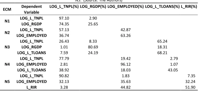
Tables 1.3 portrays the estimated impulse-response functions that trace the effects of a Cholesky one standard deviation (1 S.D.) shock to one of the endogenous variables on the other variables of VEC models N1 to N5. Finally, Table 1.4 shows the respective variance decomposition, which provides information about the relative importance of each

random innovation in affecting the variables in the VECs. For model N2, over a forecast horizon of 10 quarters (2.5 years), up to 57 percent of the forecast error variance in the LOG_L_TNPL variable can be explained by its own shocks, with the remaining 43 percent being due to shocks in the other variable (herein, LOG_EMPLOYED).

Table 1.3 Impulse Response Analyses to Cholesky’s one s.d. shock in ten Quarters ahead for Error Correction Models N1 to N5. (Source: The Authors)

ECM Dependent Variable

LOG_L_TNPL(%) LOG_RGDP(%) LOG_EMPLOYED(%) LOG_L_TLOANS(%) L_RIR(%)

N1 LOG_L_TNPL 0.11 0.00 LOG_RGDP -0.02 0.00 N2 LOG_L_TNPL 0.07 -0.09 LOG_EMPLOYED -0.02 0.03 N3 LOG_L_TNPL 0.03 -0.03 0.09 LOG_RGDP 0.00 0.02 -0.02 LOG_L_TLOANS 0.01 0.03 0.02 N4 LOG_L_TNPL 0.02 -0.03 0.00 LOG_EMPLOYED 0.01 0.04 0.00 LOG_L_TLOANS -0.05 0.04 0.05 N5 LOG_L_TNPL 0.11 -0.01 0.04 LOG_EMPLOYED -0.02 0.01 -0.01 L_RIR -0.34 -0.92 0.90

Table 1.4 Variance Decomposition Analyses in ten Quarters ahead for Error Correction Models N1 to N5. (Source: The Authors)

ECM Dependent Variable

LOG_L_TNPL(%) LOG_RGDP(%) LOG_EMPLOYED(%) LOG_L_TLOANS(%) L_RIR(%)

N1 LOG_L_TNPL 97.10 2.90 LOG_RGDP 74.35 25.65 N2 LOG_L_TNPL 57.13 42.87 LOG_EMPLOYED 36.74 63.26 N3 LOG_L_TNPL 26.43 8.33 65.24 LOG_RGDP 1.01 80.69 18.31 LOG_L_TLOANS 7.59 24.19 68.21 N4 LOG_L_TNPL 77.79 19.42 2.79 LOG_EMPLOYED 2.81 96.12 1.07 LOG_L_TLOANS 38.92 18.03 43.05 N5 LOG_L_TNPL 90.82 1.83 7.35 LOG_EMPLOYED 32.13 35.63 32.24 L_RIR 3.28 44.82 51.90

5.2 VAR representation

This section discusses the estimates of our vector autoregression (VAR) models, which analyze the dynamic impact of random disturbances on systems incorporating various combinations of the variables under examination. Compared to the data panel estimation techniques that have been extensively used in the literature to analyze the determinants of non-performing loans, the VAR methodology has the advantage of addressing the issue of potential endogeneity (by treating all variables as endogenous) and of fully capturing the dynamic interactions between the different types of determinants.

The variables utilized in the analysis presented in this section include:

TNPL: ratio of the aggregate (banking sector-wide) outstanding stock of non-performing loans including restructured loans to the total outstanding stock of loans provided by Greek credit institutions.

TNPL_CONS; TNPL_HOUSE; and TNPL_CORP represent the respective

ratios for consumer, mortgage and corporate non-performing loans including restructured loans.

L_RESTRUCT: ratio of the total stock of restructured loans (all types of

loans).

RGDP: realGDP growth (quarterly);

RHP:realgrowth of housing prices (quarterly);

UNPL: Greece’s unemployment rate as a percent of the total labour

force.

EMPLOYED: quarterly growth of the total number of employed persons.

INFL: quarterly growth of the harmonized consumer price index for Greece.

L_RIR: real interest rate on bank loans (calculated using as weights the outstanding volumes of domestic monetary financial institutions’ loans vis-à-vis euro area private-sector residents). L_CONS_RIR, L_HOUSE_RIR

and L_CORP_RIR are the respective acronyms for the real interest rate

on consumer, mortgage and corporate loans.

LD_IRS:loans-to-deposits interest rate spread.

PERFO_TL_RG; PERFO_CONS_RG, PERFO_HOUSE_RG and

PERFO_CORP_RG): respective real quarterly growth of the stock of

total, consumer, mortgage and corporate performing loans (net of provisions).

ETA: solvency ratio (banking sector-wide), measured as total common shareholders equity to total bank assets.

C12: crisis dummy taking the value of 1 from Q1 2012 onwards and 0 otherwise.

C13: dummy variable taking the value 1 in Q1 2013 and the value zero in all other quarters.

In our VAR model specifications, some of the above variables enter in first differences so as to address any non-stationarity issues (variables in first differences are preceded by the letter D). For instance, D(TNPL) denoted the quarterly change in the ratio of non-performing loans including restructured loans.

All estimated VAR models presented in this sector pass the usual diagnostic tests as regards model specification and stability, selected lag length as well as residual autocorrelation, heteroscedasticity and

5.2.1 NPL VARs with macro determinants

The estimates of our VAR models for the ratio of total NPLs including restructured loans (all sectors) as well as for the respective ratios for consumer, mortgage and corporate loans are reported in Tables 2.1 to 2.4. The results of a series of relevant causality tests are also reported in the aforementioned tables, confirming the efficacy of the models under examination. In most cases, the estimated coefficients have the correct theoretical sign and are statistically significant.

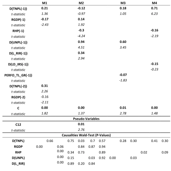
Table 2.1 Estimated VAR models for aggregate non-performing loans (Source: The Authors)

M1 M2 M3 M4 D(TNPL(-1)) 0.21 -0.12 0.18 0.71 t-statistic 1.36 -0.97 1.05 6.23 RGDP(-1) -0.17 0.14 t-statistic -2.43 1.92 RHP(-1) -0.3 -0.16 t-statistic -4.24 -2.19 D(UNPL(-1)) 0.94 0.60 t-statistic 4.51 3.45 D(L_RIR(-1)) 0.34 t-statistic 2.94 D(LD_IRS(-1)) -0.15 t-statistic -0.23 PERFO_TL_GR(-1)) -0.07 t-statistic -1.83 D(TNPL(-2)) 0.31 t-statistic 2.26 RGDP(-2) -0.16 t-statistic -2.11 C 0.00 0.00 0.01 0.00 t-statistic 1.82 1.37 2.78 1.48 Pseudo-Variables C12 0.01 t-statistic 2.76

Causalities Wald-Test (P-Values)

D(TNPL) 0.66 0.75 0.03 0.7 0.57 0.28 0.30 0.41 0.30

RGDP 0.00 0.06 0.84 0.87 0.94

RHP 0.00 0.34 0.73 0.89 0.02 0.09

D(UNPL) 0.00 0.15 0.03 0.92 0.00 0.03

D(LD_IRS)

0.82 0.02

PERFO_TL_GR 0.07 0.55

*Variables are expressed in either ratios or growth rates

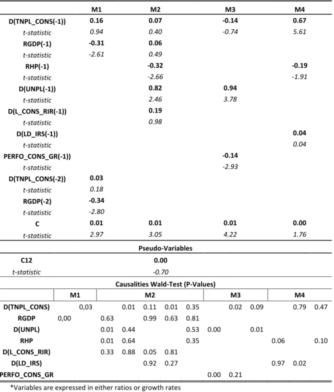
Table 2.2 Estimated VAR models for non-performing consumer loans. (Source: The Authors)

M1 M2 M3 M4 D(TNPL_CONS(-1)) 0.16 0.07 -0.14 0.67 t-statistic 0.94 0.40 -0.74 5.61 RGDP(-1) -0.31 0.06 t-statistic -2.61 0.49 RHP(-1) -0.32 -0.19 t-statistic -2.66 -1.91 D(UNPL(-1)) 0.82 0.94 t-statistic 2.46 3.78 D(L_CONS_RIR(-1)) 0.19 t-statistic 0.98 D(LD_IRS(-1)) 0.04 t-statistic 0.04 PERFO_CONS_GR(-1)) -0.14 t-statistic -2.93 D(TNPL_CONS(-2)) 0.03 t-statistic 0.18 RGDP(-2) -0.34 t-statistic -2.80 C 0.01 0.01 0.01 0.00 t-statistic 2.97 3.05 4.22 1.76 Pseudo-Variables C12 0.00 t-statistic -0.70

Causalities Wald-Test (P-Values)

M1 M2 M3 M4 D(TNPL_CONS) 0,03 0.01 0.11 0.01 0.35 0.02 0.09 0.79 0.47 RGDP 0,00 0.63 0.99 0.63 0.81 D(UNPL) 0.01 0.44 0.53 0.00 0.01 RHP 0.01 0.64 0.35 0.06 0.10 D(L_CONS_RIR) 0.33 0.88 0.05 0.81 D(LD_IRS) 0.92 0.27 0.97 0.02 PERFO_CONS_GR 0.00 0.21

*Variables are expressed in either ratios or growth rates

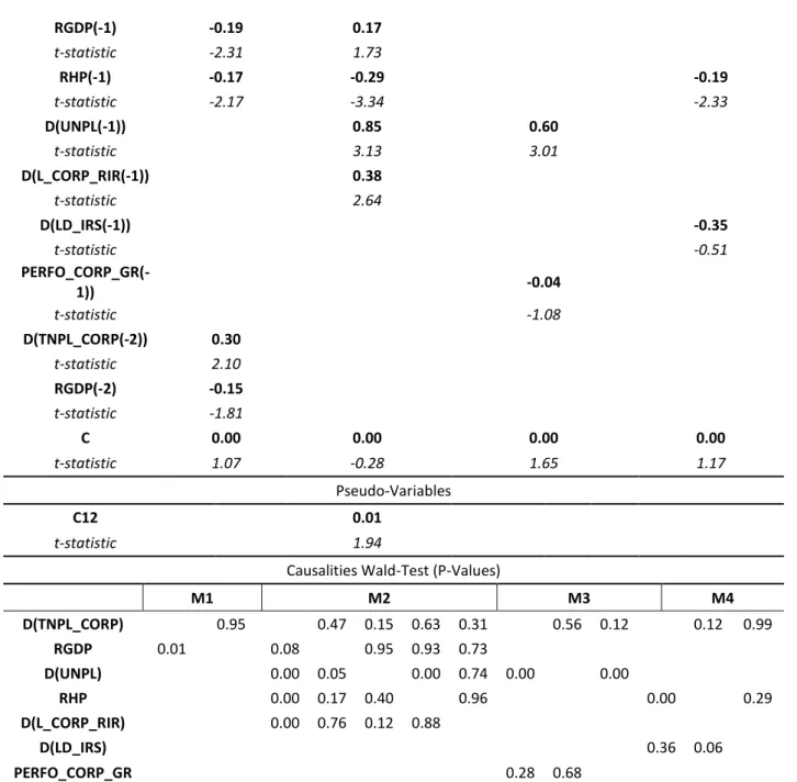
Table 2.3 Estimated VAR models for non-performing corporate loans. (Source: The Authors)

RGDP(-1) -0.19 0.17 t-statistic -2.31 1.73 RHP(-1) -0.17 -0.29 -0.19 t-statistic -2.17 -3.34 -2.33 D(UNPL(-1)) 0.85 0.60 t-statistic 3.13 3.01 D(L_CORP_RIR(-1)) 0.38 t-statistic 2.64 D(LD_IRS(-1)) -0.35 t-statistic -0.51 PERFO_CORP_GR(-1)) -0.04 t-statistic -1.08 D(TNPL_CORP(-2)) 0.30 t-statistic 2.10 RGDP(-2) -0.15 t-statistic -1.81 C 0.00 0.00 0.00 0.00 t-statistic 1.07 -0.28 1.65 1.17 Pseudo-Variables C12 0.01 t-statistic 1.94

Causalities Wald-Test (P-Values)

M1 M2 M3 M4 D(TNPL_CORP) 0.95 0.47 0.15 0.63 0.31 0.56 0.12 0.12 0.99 RGDP 0.01 0.08 0.95 0.93 0.73 D(UNPL) 0.00 0.05 0.00 0.74 0.00 0.00 RHP 0.00 0.17 0.40 0.96 0.00 0.29 D(L_CORP_RIR) 0.00 0.76 0.12 0.88 D(LD_IRS) 0.36 0.06 PERFO_CORP_GR 0.28 0.68

*Variables are expressed in either ratios or growth rates

Table 2.4 Estimated VAR models for non-performing mortgage loans. (Source: The Authors)

M1 M2 M3 M4 D(TNPL_HOUS(-1)) 0.27 0.03 0.11 0.25 t-statistic 1.71 0.17 0.58 1.62 RGDP(-1) -0.14 0.01 t-statistic -2.07 0.12 RHP(-1) -0.15 -0.21 t-statistic -1.89 -3.22 D(UNPL(-1)) 0.53 0.41 t-statistic 2.52 2.67 D(L_HOUS_RIR(-1)) 0.22 t-statistic 1.65

D(LD_IRS(-1)) 0.37 t-statistic 0.67 PERFO_HOUS_GR(-1)) -0.06 t-statistic -1.89 D(TNPL_HOUS(-2)) 0.13 t-statistic 0.89 RGDP(-2) -0.11 t-statistic -1.55 C 0.00 0.00 0.01 0.00 t-statistic 2.64 2.25 3.10 2.81 Pseudo-Variables C12 0.01 t-statistic 2.26

Causalities Wald-Test (P-Values)

M1 M2 M3 M4 D(TNPL_HOUS) 0.27 0.06 0.13 0.01 0.82 0.16 0.18 0.00 0.94 RGDP 0.04 0.90 0.90 0.90 0.91 D(UNPL) 0.01 0.15 0.75 0.82 0.01 0.25 RHP 0.06 0.67 0.67 0.85 0.00 0.28 D(L_HOUS_RIR) 0.10 0.75 0.75 0.33 D(LD_IRS) 0.50 0.00 PERFO_HOUS_GR 0.06 0.53

*Variables are expressed in either ratios or growth rates

In the VAR equations featuring non-performing loans as the left-hand side variable, the estimated coefficient of the first lag of NPLs is mostly positive, but insignificant (same result applies for models including more than one lags). The positive sign documented here is broadly in line with the findings of some earlier studies for other euro area economies; see e.g. relevant contributions for Italy by Salas and Saurina (2002); and Quagliarello (2007). The positive persistence of bad loans can be explained on the basis that it usually takes some time for NPLs to be written off banks’ balance sheets. It should be noted though that our results appear to be in some disagreement with those presented in an earlier empirical analysis on Greek NPLs conducted by Louzis et al.

the nine (9) largest Greek commercial banks spanning the period Q1 2003 to Q3 2009, these authors document a negative and significant coefficient of the lagged NPLs variable for the case of consumer and corporate loans, along with an insignificant coefficient for mortgage loans. They explain this finding on the basis that NPLs are likely to decrease when they have increased in the previous quarter, due to write-offs. On the other hand, they interpret the insignificant coefficient for lagged mortgage NPLs as evidence supporting the view that macro fundamentals play a greater role in driving this particular category of bad debts. Overall, we would not be overly concerned about this deviation of empirical findings, given that we are using a different methodological approach. Furthermore, in contrast to Louzis et al. (2012), our study looks at aggregate (system-wide) NPL series that include restructured loans and also spans a different time period (Q1 2005 to Q4 2015).

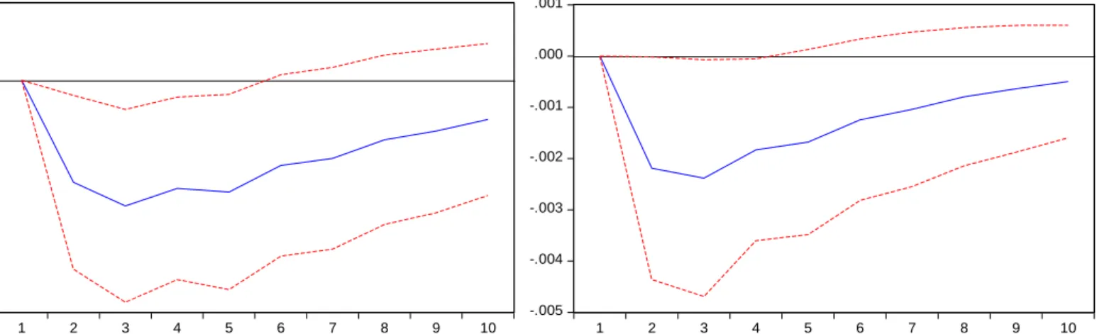
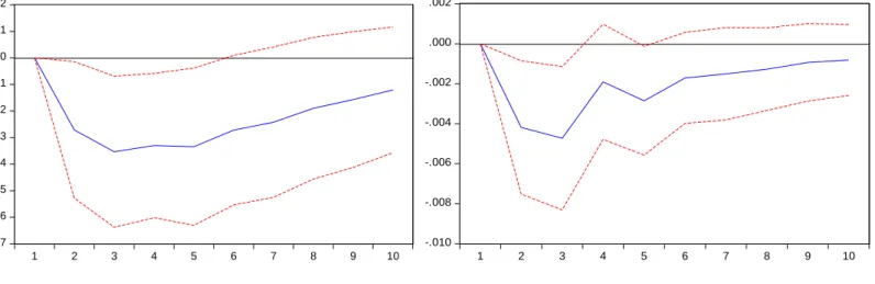
In the majority of models, the coefficient of the lagged quarterly change in the unemployment rate, D(UNPL), or, alternatively, that of the quarterly growth of total employment, EMPLOYED, has the correct theoretical sign (positive and negative, respectively) and is statistically significant. This result can be also inferred by looking at the respective impulse response functions in Figures 2.1 to 2.4. This finding is in agreement with many empirical studies in the literature (see e.g. Quagliarello, 2007; Beck et al., 2013; Klein, 2013) and its rationale is in line with the analysis presented earlier in this document (see e.g. Section 5.1). Finally, our pairwise causality tests reject both of the following null hypotheses: a) respective labour market variable does not Granger causes NPLs; and b) NPLs do not Granger cause labour market

conditions. This provides statistical evidence supporting the existence of a negative feedback effect running from NPLs to the labour market and highlights the importance of the former variable in safeguarding both financial-system and macroeconomic stability.

In a similar fashion, the coefficient(s) of lag real GDP growth is negative, though its significance diminishes in models that also include other aggregate proxies of real economic activity, such as lagged labour market variables and/or real growth of residential house prices. The finding of a negative coefficient for real GDP growth is broadly in line with what the relevant empirical literature suggests and confirms the procyclical behavior of bad loans. For instance, the estimates of a bivariate VAR for the ratio of non-performing loans and real GDP growth (model M1 in Tables 2.1 to 2.5) suggest that the transmission of GDP shocks to NPLs is relatively fast (here the maximum impact is felt within 3 quarters), with the estimated magnitude of the respective long-term impact being broadly comparable with that documented in some earlier studies. According to our estimates, a decline of real GDP growth by 1 ppt leads to a c. 0.40 ppts increase in the TNPLs ratio in the long run. Note that in their studies on the determinants of bad loans in Italy, Salas and Saurina (2002) and Quagliarello (2007) estimate a long term elasticity of c. 0.33 of NPLs with respect to GDP. Notably, our pairwise causality tests on th