Relational Abstract Domains for the
Detection of Floating-Point Run-Time Errors
?Antoine Min´e
DI-´Ecole Normale Sup´erieure de Paris, France, [email protected]
Abstract We present a new idea to adapt relational abstract domains to the analysis of IEEE 754-compliant floating-point numbers in order to statically detect, through Abstract Interpretation-based static analyses, potential floating-point run-time exceptions such as overflows or invalid operations. In order to take the non-linearity of rounding into account, expressions are modeled as linear forms with interval coefficients. We show how to extend already existing numerical abstract domains, such as the octagon abstract domain, to efficiently abstract transfer functions based on interval linear forms. We discuss specific fixpoint stabilization techniques and give some experimental results.
1
Introduction
It is a well-established fact, since the failure of the Ariane 5 launcher in 1996, that run-time errors in critical embedded software can cause great financial— and human—losses. Nowadays, embedded software is becoming more and more complex. One particular trend is to abandon fixed-point arithmetics in favor of floating-point computations. Unfortunately, floating-point models are quite com-plex and features such as rounding and special numbers (infinities,NaN, etc.) are not always understood by programmers. This has already led to catastrophic behaviors, such as the Patriot missile story told in [16].
Much work is concerned about the precision of the computations, that is to say, characterizing the amount and cause of drift between a computation on perfect reals and the corresponding floating-point implementation. Ours is not. We seek to prove that an exceptional behavior (such as division by zero or overflow) will not occur in any execution of the analyzed program. While this is a simpler problem, our goal is to scale up to programs of hundreds of thousands of lines with full data coverage and very few (even none) false alarms.
Our framework is that of Abstract Interpretation, a generic framework for designing sound static analyses that already features many instances [6,7]. We adapt existing relational numerical abstract domains (generally designed for the analysis of integer arithmetics) to cope with floating-point arithmetics. The need for such domains appeared during the successful design of a commis-sioned special-purpose prototype analyzer for a critical embedded avionics
tem. Interval analysis, used in a first prototype [3], proved too coarse because error-freeness of the analyzed code depends on tests that are inherently poorly abstracted in non-relational abstract domains. We also had to design special-purpose widenings and narrowings to compensate for the pervasive rounding errors, not only in the analyzed program, but also introduced by our efficient abstractions. These techniques were implemented in our second prototype whose overall design was presented in [4]. The present paper focuses on improvements and novel unpublished ideas; it is also more generic.
2
Related Work
Abstract Domains. A key component in Abstract-Interpretation-based anal-yses is the abstract domain which is a computer-representable class of program invariants together with some operators to manipulate them: transfer functions for guards and assignments, a control-flow join operator, and fixpoint acceler-ation operators (such as widenings Oand narrowings M) aiming at the correct and efficient analysis of loops. One of the simplest yet useful abstract domain is the widespread interval domain [6]. Relational domains, which are more precise, include Cousot and Halbwachs’s polyhedron domain [8] (corresponding to invari-ants of the form P
civi ≤c), Min´e’s octagon domain [14] (±vi±vj ≤c), and Simon’s two variables per inequality domain [15] (αvi+βvj ≤c). Even though the underlying algorithms for these relational domains allow them to abstract sets of reals as well as sets of integers, their efficient implementation—in a maybe approximate but sound way—using floating-point numbers remains a challenge. Moreover, these relational domains do not support abstracting floating-point expressions, but only expressions on perfect integers, rationals, or reals.
Floating-Point Analyses. Much work on floating-point is dedicated to the analysis of the precision of the computations and the origins of the rounding errors. The CESTAC method [17] is widely used, but also much debated as it is based on a probabilistic model of error distribution and thus cannot give sound answers. An interval-based Abstract Interpretation for error terms is proposed in [1]. Some authors [11,13] go one step further by allowing error terms to be related in relational, even non-linear, domains. Unfortunately, this extra precision does not help when analyzing programs whose correctness also depends upon relations between variables and not only error terms (such as programs with inequality tests, as in Fig. 3).
Our Work. We first present our IEEE 754-based computation model (Sect. 3) and recall the classical interval analysis adapted to floating-point numbers (Sect. 4). We present, in Sect. 5, an abstraction of floating-point expressions in terms of interval linear forms over the real field and use it to refine the inter-val domain. Sect. 6 shows how some relational abstract domains can be efficiently adapted to work on these linear forms. Sect. 7 presents adapted widening and narrowing techniques. Finally, some experimental results are shown in Sect. 8.
3
IEEE 754-Based Floating-Point Model
We present in this section the concrete floating-point arithmetics model that we wish to analyze and which is based on the widespread IEEE 754-1985 [5] norm.
3.1 IEEE 754 Floating-Point Numbers
The binary representation of a IEEE 754 number is composed of three fields: • a 1-bit signs;
• an exponente−bias, represented by a biasede-bit unsigned integere; • a fractionf =.b1. . . bp, represented by ap-bit unsigned integer.
The valuese,bias, andpare format-specific. We will denote byFthe set of all available formats and byf =32the 32-bitsingleformat (e= 8, bias= 127, andp= 23). Floating-point numbers belong to one of the following categories:
• normalizednumbers (−1)s×2e−bias×1.f, when 1≤e≤2e−2;
• denormalizednumbers (−1)s×21−bias×0.f, whene= 0 andf 6= 0;
• +0 or−0 (depending ons), whene= 0 andf = 0; • +∞or−∞(depending ons), whene= 2e−1 andf = 0;
• error codes (so-calledNaN), whene= 2e−1 and f 6= 0.
For each formatf ∈Fwe define in particular: • mff = 2
1−bias−pthe smallest non-zero positive number;
• Mff = (2−2−p)2
2e
−bias−2, the largest non-infinity number.
The special values +∞ and−∞may be generated as a result of operations undefined onR(such as 1/+0), or when a result’s absolute value overflowsMff.
Other undefined operations (such as +0/+0) result in a NaN (that stands for Not A Number). The sign of 0 serves only to distinguish between 1/+0 = +∞ and 1/−0 =−∞; +0 and −0 are indistinguishable in all other contexts (even comparison).
Due to the limited number of digits, the result of a floating-point operation needs to be rounded. IEEE 754 provides four rounding modes: towards 0, towards +∞, towards−∞, and to nearest. Depending on this mode, either the floating-point number directly smaller or directly larger than the exact real result is chosen (possibly +∞or −∞). Rounding can build infinities from non-infinities operands (this is called overflow), and it may return zero when the absolute value of the result is too small (this is calledunderflow). Because of this rounding phase, most algebraic properties of R, such as associativity and distributivity, are lost. However, the opposite of a number is always exactly represented (unlike what happens in two-complement integer arithmetics), and comparison operators are also exact. See [10] for a description of the classical properties and pitfalls of the floating-point arithmetics.
3.2 Custom Floating-Point Computation Model
We focus our analysis on the large class of programs that treat floating-point arithmetics as a practical approximation to the mathematical realsR: roundings and underflows are tolerated, but not overflows, divisions by zero or invalid operations, which are considered run-time errors and halt the program. Our goal is to detect such behaviors. In this context, +∞,−∞, andNaNs can never
Rf,+∞(x) = ½ Ω ifx >Mff min{y∈Ff|y≥x} otherwise Rf,−∞(x) = ½ Ω ifx <−Mff max{y∈Ff |y≤x} otherwise Rf,0(x) = ½ min{y∈Ff|y≥x} ifx≤0 max{y∈Ff |y≤x} ifx≥0 Rf,n(x) = Ω if|x| ≥(2−2−p−1 )22e−bias−2 Mff else ifx≥Mff −Mff else ifx≤ −Mff Rf,−∞(x) else if|Rf,−∞(x)−x|<|Rf,+∞(x)−x| Rf,+∞(x) else if|Rf,+∞(x)−x|<|Rf,−∞(x)−x|
Rf,−∞(x) else ifRf,−∞(x)’s least significant bit is 0
Rf,+∞(x) else ifRf,+∞(x)’s least significant bit is 0
Figure 1.Rounding functions, extracted from [5].
Jconstf,r(c)Kρ=Rf,r(c) JvKρ =ρ(v) Jcastf,r(e)Kρ =Rf,r(JeKρ) ifJeKρ6= Ω Je1¯f,re2Kρ =Rf,r((Je1Kρ)·(Je2Kρ)) ifJe1Kρ,Je2Kρ6= Ω, · ∈ {+,−,×} Je1®f,re2Kρ =Rf,r((Je1Kρ)/(Je2Kρ)) ifJe1Kρ6= Ω, Je2Kρ /∈ {0,Ω} JªeKρ =−(JeKρ) ifJeKρ6= Ω
JexprfKρ = Ω in all other cases
Figure 2.Expression concrete semantics, extracted from [5].
be created and, as a consequence, the difference between +0 and −0 becomes irrelevant. For every format f ∈ F, the set of floating-point numbers will be assimilated to a finite subset ofRdenoted byFf. The grammar of floating-point
expressions of format f includes constants, variables v ∈ Vf of formatf, casts
(conversion from another format), binary and unary arithmetic operators (circled in order to distinguish them from the corresponding operators on reals):
exprf :==constf,r(c) c∈R
| v v∈ Vf
| castf,r(exprf0)
| exprf¯f,rexprf ¯ ∈ {⊕,ª,⊗,®}
| ªexprf
Some constructs are tagged with a floating-point formatf ∈Fand a round-ing moder ∈ {n,0,+∞,−∞} (nrepresenting rounding to nearest). A notable exception is the unary minusªwhich does not incur rounding and never results in a run-time error as all theFfs are perfectly symmetric.
An environmentρ ∈ Q
f∈F(Vf → Ff) is a function that associates to each
variable a floating-point value of the corresponding format. Fig. 2 gives the concrete semantics JexprfKρ ∈ Ff ∪ {Ω} of the expression exprf in the
solely the regular operators +,−,×,/on real numbers and the rounding function Rf,r :R→Ff ∪ {Ω} defined in Fig. 1. It corresponds exactly to the IEEE 754
norm [5] where the overflow, division by zero, and invalid operation exception traps abort the system with a run-time error.
4
Floating-Point Interval Analysis
Floating-Point Interval Arithmetics. The idea of interval arithmetics is to over-approximate a set of numbers by an interval represented by its lower and upper bounds. For each format f, we will denote by If the set of real intervals
with bounds inFf. AsFf is totally ordered and bounded, any subset of Ff can
be abstracted by an element ofIf. Moreover, as all rounding functionsRf,r are
monotonic, we can compute the bounds of any expression using pointing-point operations only, ensuring efficient implementation within an analyzer. A first idea is to use the very same format and rounding mode in the abstract as in the concrete, which would give, for instance, the following addition (Ω denoting a run-time error): [a−;a+]⊕] f,r[b −;b+] = ½ Ω ifa−⊕ f,rb−= Ω ora+⊕f,rb+= Ω [a−⊕ f,rb−;a+⊕f,rb+] otherwise
A drawback of this semantics is that it requires the analyzer to determine, for each instruction, which rounding moderand which formatf are used. This may be difficult as the rounding mode can be changed at run-time by a system call, and compilers are authorized to perform parts of computations using a more precise IEEE format that what is required by the programmer (on Intel x86, all floating-point registers are 80-bit wide and rounding to the user-specified format occurs only when the results are stored into memory). Unfortunately, using in the abstract a floating-point format different from the one used in the concrete computation is not sound.
The following semantics, inspired from the one presented in [11], solves these problems by providing an approximation that is independent from the concrete rounding mode (assuming always the worst: towards −∞ for the lower bound and towards +∞for the upper bound):
•const]f(c) = [constf,−∞(c);constf,+∞(c)] •cast]f(c) = [castf,−∞(c);castf,+∞(c)] •[a−;a+ ]⊕]f [b −;b+ ] = [a−⊕ f,−∞b−;a+⊕f,+∞b+] •[a−;a+]ª] f [b −;b+] = [a−ª f,−∞b+;a+ªf,+∞b−] •[a−;a+]⊗] f [b −;b+] = [min((a+⊗ f,−∞b+),(a−⊗f,−∞b+),(a+⊗f,−∞b−),(a−⊗f,−∞b−)); max((a+⊗ f,+∞b+),(a−⊗f,+∞b+),(a+⊗f,+∞b−),(a−⊗f,+∞b−))] •[a−;a+]®] f [b −;b+] = ◦Ω ifb−≤0≤b+ ◦[min((a+ ®f,−∞b+),(a−®f,−∞b+),(a+®f,−∞b−),(a−®f,−∞b−)); max((a+ ®f,+∞b+),(a−®f,+∞b+),(a+®f,+∞b−),(a−®f,+∞b−))]
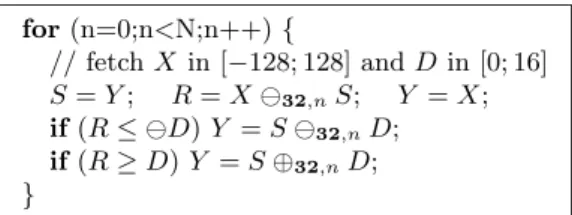
for(n=0;n<N;n++){ // fetchX in [−128; 128] andD in [0; 16] S=Y; R=Xª32,nS; Y =X; if(R≤ ªD)Y =Sª32,nD; if(R≥D)Y =S⊕32,nD; }
Figure 3. Simple rate limiter function with inputX, output Y, and maximal rate variationD.
otherwise • ª][a−;a+
] = [ªa+ ;ªa−]
•return Ω if one interval bound evaluates to Ω
This semantics frees the analyzer from the job of statically determining the rounding mode of the expressions and allows the analyzer to use, in the abstract, less precise formats that those used in the concrete (however, using a more precise format in the abstract remains unsound).
Floating-Point Interval Analysis. Interval analysis is a non-relational Ab-stract Interpretation-based analysis where, at each program point and for each variable, the set of its possible values during all executions reaching this point is over-approximated by an interval. An abstract environment ρ] is a func-tion mapping each variable v ∈ Vf to an element of If. The abstract value
JexprfK]ρ]∈If ∪ {Ω} of an expressionexprf in an abstract environment ρ]can
be derived by induction using the interval operators defined in the preceding paragraph.
An assignmentv←exprf performed in an environmentρ] returnsρ] where
v’s value has been replaced byJexprfK]ρ]if it does not evaluate to Ω, and
other-wise byFf (thetopvalue) and reports an error. Most tests can only be abstracted
by ignoring them (which is sound). Even though for simple tests such as, for in-stance, X ≤ Y ⊕f,rc, the interval domain is able to refine the bounds for X
and Y, it cannot remember the relationship between these variables. Consider the more complete example of Fig. 4. It is a rate limiter that given random in-put flows X and D, bounded respectively by [−128; 128] and [0; 16], computes an output flow Y that tries to follow X while having a change rate limited by D. Due to the imprecise abstraction of tests, the interval domain will boundY by [−128−16n; 128 + 16n] after n loop iterations while in fact it is bounded by [−128; 128] independently from n. IfN is too big, the interval analysis will conclude that the limiter may overflow while it is in fact always perfectly safe.
5
Linearization of Floating-Point Expressions
Unlike the interval domain, relational abstract domains rely on algebraic proper-ties of operators, such as associativity and distributivity, that are not true in the floating-point world. Our solution is to approximate floating-point expressions bylinear expressionsin therealfield withinterval coefficientsand free variables in V =∪f∈FVf. Leti+Pv∈Vivv be such a linear form; it can be viewed as a function fromRV to the set of real intervals. For the sake of efficiency, interval
coefficient bounds will be represented by floating-point numbers in a format fa
that is efficient on the analyzer’s platform: i, iv ∈ Ifa. Because, for all f and
· ∈ {+,−,×, /}, ¯]f is a valid over-approximation of the corresponding real
in-terval arithmetics operation, we can define the following sound operators¢],¯],
£],¾] on linear forms: •(i+P v∈Vivv)¢ ](i0+P v∈Vi 0 vv) = (i⊕ ] fai 0) +P v∈V(iv⊕ ] fai 0 v)v •(i+P v∈Vivv)¯ ](i0+P v∈Vi 0 vv) = (iª]fai0) + P v∈V(ivª ] fai0v)v •i£](i0+P v∈Vi 0 vv) = (i⊗ ] fai 0) +P v∈V(i⊗ ] fai 0 v)v •(i+P v∈Vivv)¾]i 0 = (i®] fai 0) +P v∈V(iv® ] fai 0)v
Given an expression exprf and an interval abstract environment ρ] as in
Sect. 4, we construct the interval linear formLexprfMρ] onV as follows:
•Lconstf,r(c)Mρ] = [constf,−∞(c);constf,+∞(c)] •LvfMρ] = [1; 1]vf •Lcastf,r(e)Mρ] =LeMρ] ¢] εf(LeMρ]) ¢] mff[−1; 1] •Le1⊕f,re2Mρ] = Le1Mρ] ¢] Le2Mρ] ¢] ε f(Le1Mρ]) ¢] εf(Le2Mρ]) ¢] mff[−1; 1] •Le1ªf,re2Mρ] = Le1Mρ] ¯] Le2Mρ] ¢] ε f(Le1Mρ]) ¢] εf(Le2Mρ]) ¢] mff[−1; 1] •L[a;b]⊗f,re2Mρ]= ([a;b]£]Le2Mρ]) ¢] ([a;b]£]ε f(Le2Mρ])) ¢] mff[−1; 1] •Le1⊗f,r[a;b]Mρ]=L[a;b]⊗f,re1Mρ] •Le1⊗f,re2Mρ] =Lι(Le1Mρ])ρ] ⊗f,r e2Mρ] •Le1®f,r[a;b]Mρ]= (Le1Mρ]¾][a;b]) ¢] (ε f(Le1Mρ])¾][a;b]) ¢] mff[−1; 1] •Le1®f,re2Mρ] =Le1 ®f,r ι(Le2Mρ])ρ]M
where the “error”εf(l) of the linear forml is the following linear form:
εf à [a;b] +X v∈V [av;bv]v ! = (max(|a|,|b|)⊗]fa[−2 −p; 2−p]) + X v∈V (max(|av|,|bv|)⊗]fa[−2 −p ; 2−p ])v (pis the fraction size in bits for the format f, see Sect. 3.1)
and the “intervalization”ι(l)ρ] function over-approximates the range of the linear forml in the abstract environmentρ]as the following interval ofI
fa: ι à i+X v∈V ivv ! ρ]=i⊕] fa à M] fa v∈V iv⊗]faρ](v) !
(any summation order for ⊕]fa is sound)
Note that this semantics is very different from the one proposed by Goubault in [11] and subsequently used in [13]. In [11], each operation introduces a new variable representing an error term, and there is no need for interval coefficients.
About ι. Dividing a linear form by another linear form which is not reduced to an interval does not yield a linear form. In this case, theιoperator is used to over-approximate the divisor by a single interval before performing the division. The same holds when multiplying two linear forms not reduced to an interval, but we can choose to applyιto either argument. For the sake of simplicity, we chose here to “intervalize” the left argument. Moreover, any non-linear operator (such as, e.g., square root or sine) could be dealt with by performing the corresponding operator on intervals after “intervalizing” its argument(s).
Aboutεf. To account for rounding errors, an upper bound of|Rf,r(x·y)−(x·y)|
(where· ∈ {+,−,×, /}) is included inLexprfMρ]. It is the sum an error relative
to the argumentsxandy, expressed usingεf, and an absolute errormff due to
a possible underflow. Unlike what happened with interval arithmetics, correct error computation does not require the abstract operators to use floating-point formats that are no more precise than the concrete ones: the choice of fa is completely free.
About Ω. It is quite possible that, during the computation of LexprfMρ], a
floating-point run-time error Ω occurs. In that case, we will say that the lin-earization “failed”. It does not mean that the program has a run-time error, but only that we cannot compute a linearized expression and must revert to the classical interval arithmetics.
Main Result. When we evaluate in Rthe linear formLexprfMρ]in a concrete
environmentρ included inρ] we get a real interval that over-approximates the concrete value of the expression:
Theorem 1.
If JexprfK]ρ]6= Ωand the linearization does not fail and ∀v∈ V, ρ(v)∈ρ](v),
thenJexprfKρ∈LexprfMρ](ρ).
Linear Form Propagation. As the linearization manipulates expressions sym-bolically, it is able to perform simplifications when the same variable appears several times. For instance Z ←Xª32,n(0.25⊗32,nX) will be interpreted as Z ←[0.749· · · ; 0.750· · ·]X+ 2.35· · ·10−38[−1; 1]. Unfortunately, no simplifica-tion can be done if the expression is broken into several statements, such as in Y ←0.25⊗32,nX;Z ← Xª32,nY. Our solution is to remember, in an extra environmentρ]l, the linear form assigned to each variable and use this informa-tion while linearizing: we setLvfM(ρ], ρl]) =ρ]l(v) instead of [−1; 1]vf. Care must
be taken, when a variable v is modified, to discard all occurrences of v in ρ]l. Effects of tests onρ]l are ignored. Our partial order on linear forms is flat, so, at control-flow joins, only variables that are associated with the same linear form in both environments are kept; moreover, we do not need any widening. This technique is reminiscent of Kildall’s constant propagation [12].
Applications. A first application of linearization is to improve the preci-sion of the interval analysis. We simply replace JexprfK]ρ] by JexprfK]ρ] ∩
While improving the assignment transfer function (trough expression simpli-fication), this is not sufficient to treat tests precisely. For this, we need relational domains. Fortunately, Thm. 1 also means that if we have a relational domain that manipulates sets of points with real coordinates RV and that is able to perform assignments and tests of linear expressions with interval coefficients, we can use it to perform relational analyses on floating-point variables. Consider, for instance, the following algorithm to handle an assignmentv←exprf in such
a relational domain (the procedure would be equivalent for tests):
• IfJexprfK]ρ]= Ω, then we report a run-time error and apply the transfer
function forv←Ff.
• Else, if the linearization ofexprf fails, then we do not report an error but
apply the transfer function forv←JexprfK]ρ].
• Otherwise, we do not report an error but apply the transfer function for v←LexprfMρ].
Remark how we use the interval arithmetics to perform the actual detection of run-time errors and as a fallback when the linearization cannot be used.
6
Adapting Relational Abstract Domains
We first present in details the adaptation of the octagon abstract domain [14] to use floating-point arithmetics and interval linear forms, which was implemented in our second prototype analyzer [4]. We then present in less details some ideas to adapt other domains.
6.1 The Octagon Abstract Domain
The octagon abstract domain [14] can manipulate sets of constraints of the form ±x±y ≤c,x, y ∈ V, c ∈E where E can be Z, Q, or R. An abstract element
ois represented by a half-square constraint matrix of size|V|. Each element at line i, column j withi ≤j contains four constraints: vi+vj ≤c, vi−vj ≤c, −vi+vj ≤c, and−vi−vj≤c, withc∈E=E∪ {+∞}. Remark that diagonal elements represent interval constraints as 2vi ≤cand−2vi ≤c. In the following, we will use notations such as maxo(vi+vj) to access the upper bound, inE, of
constraints embedded in the octagon o.
Because constraints in the matrix can be combined to obtain implied con-straints that may not be in the matrix (e.g., fromx−y ≤c andy+z≤d, we can deduce x+z ≤c+d), two matrices can represent the same set of points. We introduced in [14] a Floyd-Warshall-based closure operator that provides a normal form by combining and propagating, inO(|V|3
) time, all constraints. The optimality of the abstract operators requires to work on closed matrices.
Floating-Point Octagons. In order to represent and manipulate efficiently constraints on real numbers, we choose to use floating-point matrices: Ffa
re-placesE(wherefais, as before, an efficient floating-point format chosen by the analyzer implementation). As the algorithms presented in [14] make solely use of the + and≤operators onE, it is sufficient to replace + by⊕fa,+∞ and map Ω to +∞in these algorithms to provide a sound approximation of all the transfer
functions and operators on reals using only Ffa =Ffa∪ {+∞}. As all the nice
properties ofEare no longer true inFfa, the closure is no longer a normal form.
Even though working on closed matrices will no longer guaranty the optimality of the transfer functions, it still greatly improves their precision.
Assignments. Given an assignment of the form vk ← l, where l is a interval linear form, on an octagono, the resulting set is no always an octagon. We can choose between several levels of approximation. Optimality could be achieved at great cost by performing the assignment in a polyhedron domain and then computing the smallest enclosing octagon. We propose, as a less precise but much faster alternative (O(|V|time cost), to replace all constraints concerning the variablevk by the following ones:
vk+vi ≤u(o, l¢]vi) ∀i6=k vk−vi ≤u(o, l¯]vi) ∀i6=k −vk+vi≤u(o, vi¯]l) ∀i6=k −vk−vi≤u(o,¯](l¢]vi)) ∀i6=k vk ≤u(o, l) −vk ≤u(o,¯]l)
where the upper bound of a linear forml on an octagon ois approximated byu(o, l)∈Ffa as follows: u à o, [a−;a+ ] +X v∈V [a− v;a + v]v ! =a+ ⊕fa,+∞ M fa,+∞ v∈V
max( maxo(v)⊗fa,+∞a+v, ª(maxo(−v)⊗fa,−∞a+v), maxo(v)⊗fa,+∞a−v, ª(maxo(−v)⊗fa,−∞a−v))
(any summation order for ⊕fa,+∞ is sound)
and⊕fa,+∞ and⊗fa,+∞ are extended toFfa as follows:
+∞ ⊕fa,+∞x=x⊕fa,+∞+∞= +∞ +∞ ⊗fa,+∞x=x⊗fa,+∞+∞=
½
0 ifx= 0 +∞ otherwise
Example 1. Consider the assignment X = Y ⊕32,nZ with Y, Z ∈ [0; 1]. It is linearized as X = [1−2−23
; 1 + 2−23
](Y +Z) +mf32[−1; 1], so our abstract
transfer function will infer relational constraints such asX−Y ≤1+2−22
+mf32.
Tests. Given a test of the forml1≤l2, wherel1 andl2 are linear forms, for all variable vi 6=vj, appearing in l1 or l2, the constraints in the octagonocan be tightened by adding the following extra constraints:
vj−vi ≤u(o, l2¯]l1¯]vi¢]vj) vj+vi ≤u(o, l2¯]l1¢]vi¢]vj) −vj−vi≤u(o, l2¯]l1¯]vi¯]vj) −vj+vi≤u(o, l2¯]l1¢]vi¯]vj) vi ≤u(o, l2¯]l1¢]vi)
−vi≤u(o, l2¯]l1¯]vi)
Example 2. Consider the testY⊕32,nZ≤1 withY, Z∈[0; 1]. It is linearized as [1−2−23
; 1 + 2−23
](Y+Z) +mf32[−1; 1]≤[1; 1]. Our abstract transfer function
will be able to infer the constraint:Y +Z≤1 + 2−22
+mf32.
Example 3. The optimal analysis of the rate limiter function of Fig. 3 would require representing interval linear invariants on three variables. Nevertheless, the octagon domain with our approximated transfer functions can prove that the output Y is bounded by [−136; 136] independently fromn (the optimal bound being [−128; 128]), which is sufficient to prove thatY does not overflow.
Reduction with Intervals. The interval environmentρ]is important as we use it to perform run-time error checking and to compute the linear form associated to an expression. So, we suppose that transfer functions are performed in parallel in the interval domain and in the octagon domain, and then, information from the octagon result ois used to refine the interval resultρ] as follows: for each variablev∈ V, the upper bound ofρ](v) is replaced by min(maxρ](v),max
o(v))
and the same is done for its lower bound.
6.2 Polyhedron Domain
The polyhedron domain is much more precise than the octagon domain as it al-lows manipulating sets of invariants of the form P
vcvv≤c, but it is also much more costly. Implementations, such as the New Polka or the Parma Polyhedra libraries [2], are targeted at representing sets of points with integer or ratio-nal coordinates. They interratio-nally use ratioratio-nal coefficients and, as the coefficients usually become fairly large, arbitrary precision integer libraries.
Representing Reals. These implementations could be used as-is to abstract sets of points with real coordinates, but the rational coefficients may get out of control, as well as the time cost. Unlike what happened for octagons, it is not so easy to adapt the algorithms to floating-point coefficients while retaining soundness as they are much much more complex. We are not aware, at the time of writing, of any such floating-point implementation.
Assignments and Tests. Assignments of the formv←land tests of the form l ≤0 wherel = [a−;a+] +P
v∈V[a −
v;a+v]v seem difficult to abstract in general. However, the case where all coefficients inlare scalar except maybe the constant one is much easier. To cope with the general case, an idea (yet untested) is to use the following transformation that abstracts l into an over-approximated linear forml0 where∀v, a−
v =a +
v by transforming all relative errors into absolute ones:
l0= Ã [a−;a+ ]⊕]fa M] fa v∈V (a+ v ªfa,+∞a−v)⊗ ] fa[0.5; 0.5]⊗ ] faρ ](v) ! + X v∈V ((a− v ⊕fa,+∞a+v)⊗ ] fa[0.5; 0.5])v
6.3 Two Variables per Linear Inequalities Domain
Simon’s domain [15] can manipulate constraints of the form αvi +βvj ≤ c, α, β, c ∈ Q. An abstract invariant is represented using a planar convex poly-hedron for each pair of variables. As for octagons, most computations are done point-wise on variable pairs and a closure provides the normal form by propagat-ing and combinpropagat-ing constraints. Because the underlypropagat-ing algorithms are simpler than for generic polyhedra, adapting this domain to handle floating-point com-putations efficiently may prove easier while greatly improving the precision over octagons. This still remains an open issue.
6.4 Ellipsoid and Digital Filter Domains
During the design of our prototype analyzer [4], we encountered code for comput-ing recursive sequences such asXi= ((α⊗32,nXi−1)⊕32,n(β⊗32,nXi−2))⊕32,nγ
(1), or Xi = (α⊗32,nXi−1)⊕32,n(Yiª32,nYi−1) (2). In order to find precise bounds for the variable X, one has to consider invariants out of the scope of classical relational abstract domains. Case (1) can be solved by using the el-lipsoid abstract domain of [4] that can represent non-linear real invariants of the form aX2
i +bX 2
i−1+cXiXi−1 ≤ d, while case (2) is precisely analyzed using Feret’s filter domains [9] by inferring temporal invariants of the form |Xi| ≤ amaxj≤i|Yj|+b. It is not our purpose here to present these new ab-stract domains but we stress the fact that such domains, as the ones discussed in the preceding paragraphs, are naturally designed to work with perfect reals, but used to analyze imperfect floating-point computations.
A solution is, as before, to design these domains to analyze interval linear assignments and tests on reals, and feed them with the result of the linearization of floating-point expressions defined in Sect. 5. This solution has been successfully applied (see [9] and Sect. 8).
7
Convergence Acceleration
In the Abstract Interpretation framework, loop invariants are described as fix-points and are over-approximated by iterating, in the abstract, the body transfer function F] until a post-fixpoint is reached.
Widening. The wideningOis a convergence acceleration operator introduced in [6] in order to reduce the number of abstract iterations: limi(F])i is replaced by limiEi] whereE ] i+1=E ] i OF](E ]
i). A straightforward widening on intervals and octagons is to simply discard unstable constraints. However, this strategy is too aggressive and fails to discover sequences that are stable after a certain bound, such as, e.g., X = (α⊗32,nX)⊕32,nβ. To give these computations a chance to stabilize, we use a staged widening that tries a user-supplied set of bounds in increasing order. As we do not know in advance which bounds will be stable, we use, as setTof thresholds, a simple exponential ramp:T={±2i}∩F
fa.
Given two octagonsoando0, the widening with thresholdsoOo0 is obtained by setting, for each binary unit expression±vi±vj:
maxoOo0(C) =
½
maxo(C) if maxo0(C)≤maxo(C) min{t∈T∪ {+∞} |t≥maxo0(C)}otherwise
Decreasing Iterations. We now suppose that we have iterated the widening with thresholds up to an abstract post-fixpointX]: F](X])vX]. The bound of a stable variable is generally over-approximated by the threshold immediately above. One solution to improve such a bound is to perform some decreasing iterations Xi+1] =Xi]uF(Xi]) fromX0]=X]. We can stop whenever we wish, the result will always be, by construction, an abstraction of the concrete fixpoint; however, it may no longer be a post-fixpoint forF]. It is desirable for invariants to be abstract post-fixpoint so that the analyzer can check them independently from the way they were generated instead of relying solely on the maybe buggy fixpoint engine.
Iteration Perturbation. Careful examination of the iterates on our bench-marks showed that the reason we do not get an abstract post-fixpoint is that the abstractcomputations are done in floating-point which incurs a somewhat non-deterministic extra rounding. There exists, betweenF]’s definitive pre-fixpoints and F]’s definitive post-fixpoints, a chaotic region. To ensure that theX]
i stay above this region, we replace the intersectionuused in the decreasing iterations by the following narrowingM:oMo0 =²(ouo0) where²(o) returns an octagon where the bound of each unstable constraint is enlarged by²×d, wheredis the maximum of all non +∞constraint bounds in o. Moreover, replacingoOo0 by ²(oOo0) allows the analyzer to skip aboveF]’s chaotic regions and effectively reduces the required number of increasing iterations, and so, the analysis time.
Theoretically, a good²can be estimated by the relative amount of rounding errors performed in the abstract computation of one loop iteration, and so, is a function of the complexity of the analyzed loop body, the floating-point formatfa
used in the analyzer and the implementation of the abstract domains. We chose to fix ² experimentally by enlarging a small value until the analyzer reported it found an abstract post-fixpoint for our program. Then, as we improved our abstract domains and modified the analyzed program, we seldom had to adjust this²value.
8
Experimental Results
We now show how the presented abstract domains perform in practice. Our only real-life example is the critical embedded avionics software of [4]. It is a 132,000 lines reactive C program (75 KLoc after preprocessing) containing approximately 10,000 global variables, 5,000 of which are floating-point variables, single pre-cision. The program consists mostly of one very large loop executed 3.6·106 times. Because relating several thousands variables in a relational domain is too costly, we use the “packing” technique described in [4] to statically determine sets of variables that should be related together and we end up with approximately 2,400 octagons of size 2 to 42 instead of one octagon of size 10,000.
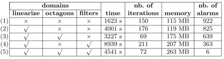
Fig. 4 shows how the choice of the abstract domains influence the precision and the cost of the analysis presented in [4] on our 2.8 GHz Intel Xeon. Together with the computation time, we also give the number of abstract executions of the big loop needed to find an invariant; thanks to our widenings and narrowings, it is much much less than the concrete number of iterations. All cases use the
domains nb. of nb. of linearize octagons filters time iterations memory alarms
(1) × × × 1623 s 150 115 MB 922
(2) √ × × 4001 s 176 119 MB 825
(3) √ √ × 3227 s 69 175 MB 639
(4) √ × √ 8939 s 211 207 MB 363
(5) √ √ √ 4541 s 72 263 MB 6
Figure 4.Experimental results.
interval domain with the symbolic simplification automatically provided by the linearization, except (1) that uses plain interval analysis. Other lines show the influence of the octagon (Sect. 6.1) and the specialized digital filter domains ([9] and Sect. 6.4): when both are activated, we only get six potential run-time errors for a reasonable run-time and memory cost. This is a sufficiently small number of alarms to allow manual inspection, and we discovered they could be eliminated without altering the functionality of the application by changing only three lines of code. Remark that as we add more complex domains, the time cost per iteration grows but the number of iterations needed to find an invariant decreases so that a better precision may reduce the overall time cost.
9
Conclusion
We presented, in this paper, an adaptation of the octagon abstract domain in order to analyze programs containing IEEE 754-compliant floating-point oper-ations. Our methodology is somewhat generic and we proposed some ideas to adapt other relational numerical abstract domains as well. The adapted octagon domain was implemented in our prototype static analyzer for run-time error checking of critical C code [4] and tested on a real-life embedded avionic ap-plication. Practical results show that the proposed method scales up well and does greatly improve the precision of the analysis when compared to the classical interval abstract domain while maintaining a reasonable cost. To our knowledge, this is the first time relational numerical domains are used to represent relations between floating-point variables.
Acknowledgments. We would like to thank all the members of the “magic” team: Bruno Blanchet, Patrick Cousot, Radhia Cousot, J´erˆome Feret, Laurent Mauborgne, David Monniaux, Xavier Rival, as well as the anonymous referees.
References
1. Y. A¨ıt Ameur, G. Bel, F. Boniol, S. Pairault, and V. Wiels. Robustness analysis of avionics embedded systems. InLCTES’03, pages 123–132. ACM Press, 2003. 2. R. Bagnara, E. Ricci, E. Zaffanella, and P. M. Hill. Possibly not closed convex
polyhedra and the Parma Polyhedra Library. In SAS’02, volume 2477 ofLNCS, pages 213–229. Springer, 2002.
3. B. Blanchet, P. Cousot, R. Cousot, J. Feret, L. Mauborgne, A. Min´e, D. Monniaux, and X. Rival. Design and implementation of a special-purpose static program analyzer for safety-critical real-time embedded software, invited chapter. InThe Essence of Computation: Complexity, Analysis, Transformation. Essays Dedicated to Neil D. Jones, LNCS, pages 85–108. Springer, 2002.
4. B. Blanchet, P. Cousot, R. Cousot, J. Feret, L. Mauborgne, A. Min´e, D. Monniaux, and X. Rival. A static analyzer for large safety-critical software. InACM PLDI’03, volume 548030, pages 196–207. ACM Press, 2003.
5. IEEE Computer Society. IEEE standard for binary floating-point arithmetic. Tech-nical report, ANSI/IEEE Std 745-1985, 1985.
6. P. Cousot and R. Cousot. Abstract interpretation: a unified lattice model for static analysis of programs by construction or approximation of fixpoints. InACM POPL’77, pages 238–252. ACM Press, 1977.
7. P. Cousot and R. Cousot. Abstract interpretation frameworks. Journal of Logic and Computation, 2(4):511–547, August 1992.
8. P. Cousot and N. Halbwachs. Automatic discovery of linear restraints among variables of a program. InACM POPL’78, pages 84–97. ACM Press, 1978. 9. J. Feret. Static analysis of digital filters. InESOP’04. LNCS, 2004.
10. D. Goldberg. What every computer scientist should know about floating-point arithmetic. ACM Computing Surveys (CSUR), 23(1):5–48, 1991.
11. ´E. Goubault. Static analyses of floating-point operations. InSAS’01, volume 2126 ofLNCS, pages 234–259. Springer, 2001.
12. G. Kildall. A unified approach to global program optimization. InPOPL’73, pages 194–206. ACM Press, 1973.
13. M. Martel. Static analysis of the numerical stability of loops. InSAS’02, volume 2477 ofLNCS, pages 133–150. Springer, 2002.
14. A. Min´e. The octagon abstract domain. InAST 2001 in WCRE 2001, IEEE, pages 310–319. IEEE CS Press, 2001.
15. A. Simon, A. King, and J. Howe. Two variables per linear inequality as an abstract domain. InLOPSTR’02, volume 2664 ofLNCS, pages 71–89. Springer, 2002. 16. R. Skeel. Roundoff error and the Patriot missile.SIAM News, 25(4):11, July 1992. 17. J. Vignes. A survey of the CESTAC method. In J-C. Bajard, editor,Proc. of Real
![Figure 2. Expression concrete semantics, extracted from [5].](https://thumb-us.123doks.com/thumbv2/123dok_us/978398.2628387/4.892.231.694.159.572/figure-expression-concrete-semantics-extracted-from.webp)