Flexible meeting scheduling

(1)

Flexible meeting scheduling

Bartłomiej Marcinowski

4th Year Project Report

Computer Science

School of Informatics

University of Edinburgh

2014

Abstract

This work presents an implementation of a library for automated meet-ing schedulmeet-ing. The solution is based on constraint logic programmmeet-ing and incorporates user preferences with the goal of finding the most suit-able meeting time. It allows users to specify the schedules and preferences of participants and finds a number of best meeting times.

(2)

(3)

Chapter 1

Introduction

1.1

Motivation

Meeting scheduling is a very common task in business as well as academia, but it is also tedious and requires a lot of time and work on behalf of the participants. Thanks to the ever expanding possibilities of computers, mobile devices and the Internet, many people now store their personal calendars online and use tools such as Google Calendar to manage their schedules. Other tools also exist for helping with the process of meet-ing schedulmeet-ing, however they still require users to manually input their availability and find the best fitting meeting times. Furthermore, they do little or nothing to allow users to distinguish between preferred and disliked slots. This project addresses this prob-lem, intending to create a software solution which can be used to shorten the meeting scheduling process and make it easier for users through leveraging technology.

1.2

Project description

The aim of the project is to develop an algorithm which will enable users to sched-ule meetings between multiple participants efficiently and easily, taking into account users’ schedules and preferences. The algorithm’s task is to find a meeting time that best suits all the participants. The users can provide the algorithm with two pieces of data: their preferences and scheduled events. The former are a concise way of describ-ing which times suit them best and which should be avoided. The user can therefore specify that they would favour meetings in the morning or that they are against meeting late in the evening. Multiple preferences can be specified simultaneously, which allows to build a complete view of the potential meeting space. The software expects to also obtain a list of each user’s events in order to discourage it from scheduling meetings during times when the user is already otherwise occupied. These events can be sourced directly from on-line calendar software, such as Google Calendar, in order to simplify the process for the user. Although the implementation of the calendar retrieval from third-party systems is not part of the task of this project, the library has been designed

(6)

to be flexible and not depend on a specific source of event data. This allows it to be used with a large variety of different calendar formats. The algorithm schedules meet-ings maximizing the total satisfaction of the group and avoids scheduling disliked or busy timeslots if possible.

The library that is the product of this work can be a useful tool for people in business and academia, who schedule meetings with multiple participants. Its usefulness in-creases with the frequency of meetings and their size (in number of participants). It is designed for users who utilize online calendar systems, although it can support events entered by hand as well.

The research hypothesis of this work is as follows: Can an automated algorithm, which uses information about scheduled events and user preferences, suggest meeting times that are satisfactory for the users? The term automated refers to two aspects of the algorithm. Firstly, the nature of its use, meaning that the user does not need to list times that suit them in order of preference. The product of this work utilizes a list of events and a list of preferences, which describes this order more concisely and can be reused between schedulings. Secondly,automatedrefers to the mechanism of finding optimal meeting times. The algorithm’s job is to review the space of possible meeting times, pick a number of best choices and present them to the user. Such an algorithm could remove the need for communicating schedules and negotiation, making meeting scheduling easier for all involved. In fact, if the meetings suggested by the algorithm are very rarely suboptimal, it could automatically schedule meetings, through entering them into the user’s calendars. However, the work done here is exploratory, so creating such a fully automated system is not the immediate goal.

1.3

Solution overview

The algorithm is a library written in Clojure, which allows it to be called both from Clojure and Java. It has been designed to be part of a larger system, which collects users’ input and displays the output back to the user. The system may also have ad-ditional functionality, such as maintaining user identities or communication between users, however this would be completely separate from the algorithm described here. It can be treated as a black box which can receive a list of events and preferences and outputs one or more meeting times which best fits the input.

The problem of finding an optimal appointment time is internally described as a con-straint optimization problem. A concon-straint solver library is then used to efficiently find a suitable solution. The algorithm input is first converted into structures which can be passed to the library and used with its constraints. The solution is then converted back into a structure which is returned and can be shown to users.

Preferences can be specified separately for each user as well as each run of the algo-rithm, which allows for flexibility in adjusting the meeting parameters by the users. This also enables the system to separate the maintenance of user data from setting up the meetings, simplifying its design.

(7)

1.4. Summary of work done 7

The evaluation performed showed that the algorithm finds suggestions which are sat-isfactory in the context of a given situation. Users can therefore utilize it to easily find a number of best meeting times for a group of people.

1.4

Summary of work done

The author carried out the following work in the course of the project: • Researching constraint satisfaction problems and libraries • Researching approaches to meeting scheduling and social choice

• Creating a software library for meeting scheduling using Constraint Logic Pro-gramming and utilizing the library chosen through research

• Implementing an original way of specifying preferences as functions of time and events

• Performing an experiment evaluating the effectiveness and suitability of the im-plemented software

1.5

Roadmap

The work is organized as follows. Chapter 2 defines the terminology used further, describes the theory relevant to this work, including constraint satisfaction problems and social choice theory and discusses a number of works in related fields. Chapter 3 contains the overview of the design of the algorithm and the outlines the reasons behind it. Chapter 4 discusses some of the more important details of the implementation of the algorithm. The methods used in the evaluation of the effectiveness of the work are described in chapter 5. The work is concluded by a summary of the results and review of possible improvements and further work.

(8)

(9)

Chapter 2

Background

2.1

Terminology

To make discussion of the work easier to understand and help disambiguate the word-ing of this paper, a brief explanation of the terminology used is presented here. When discussing meeting scheduling, themeeting windowis the period when the meeting can take place, i.e. from the first possible start time to the last possible end time. Users, or participants are the people that are scheduling a meeting and will be taking part in it. Preference values are the integer amounts that describe how much a given user wants to schedule a meeting at a particular time. These are also calledcostswhen it is more convenient to talk about them this way (e.g. when discussing the minimization of costs). Preference functionsare functions, in the software sense, which are used to check whether a given time fits a preference. The optimal meeting times which are returned by the algorithm will be termedsolutionsorsuggestions.

2.2

Meeting scheduling and social choice

In the process of scheduling a meeting, a number of people negotiate in order to decide on a single, common timeslot which fits into their schedules. As noted by Grubshtein and Meisels [14], this negotiation process requires participants to both act in their own interest (in order to fit the meeting time to their schedule), as well as cooperate with one another (in order to ensure that an agreement is reached). Social choice theory deals with the problem of ”finding a function from a set of individual preferences to a social preference order” ([13]). This is the problem that needs to be dealt with when trying to find an optimal solution to scheduling meetings with preferences.

(10)

2.3

Game-theoretic approaches to meeting scheduling

The process of scheduling a meeting can be expressed as aMeeting scheduling game. The game is played by anplayers, each of which places a bid for scheduling the ing. The bid consists of a list of preferences for each possible meeting time. The meet-ing is scheduled by choosmeet-ing a slot accordmeet-ing to itsdecision rule. Thedecision ruleis acollective utility function f:_Rn→_R, mapping a collection of player preferences to a single value which represent the global utility of the given solution.Three main types of collective utility functions, described in more detail in [15], can be distinguished:

• Utilitarian- summing of individual utilities. Maximizing this function may have the effect of decreasing the utility of one individual in order to increase another’s • Egalitarian- the minimum of individual utilities

• Nash function- product of individual utilities

This theory is important for the topic of this work, as the choice of a collective utility function for combining the preferences of individual meeting participants has a signifi-cant impact on the quality of the solutions. It is therefore important to make the choice bearing in mind the properties of the chosen function as well as the users’ perception of the problem.

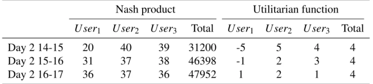
When applying game theory approaches to meeting scheduling, an analogy can be made to the bargaining problem, by observing situations where the preferences of users do not align with each other. Imagine a meeting proposition with three possible times:

t₁,t₂andt₃, two participants: p₁andp₂and preferences ranging from 1 to 10. Suppose the following preference values for the given times:

t₁ t₂ t₃ p₁ 10 1 5

p₂ 1 10 5

In this scenario, p1 prefers t1 and p2 preferst2. Therefore the users must cooperate

with each other and be able to accept a time which does not maximize their utility. Otherwise the meeting will not be scheduled at all. Using Nash’s bargaining solution and assuming the status quo utility of not scheduling the meeting to be 0, we can see that the best solution, which maximizes the product of marginal utilities (i.e. the differences between the utility of the solution and the status quo utility) is t₃, even though it is not the best for either of the players. However, a utilitarian collective utility function would rate all three solutions as equally good for the participants. This idea, and the reasoning for choosing a specific decision rule with regard to meeting scheduling, is further discussed in Section 3.3.

(11)

2.4. Constraint satisfaction problems 11

2.4

Constraint satisfaction problems

Constraint satisfaction problems (CSPs) consist of a set of variables with specified do-mains and a set of constraints on these variables, which restrict the possible values that can be assigned to each variable. Constraints can be separated into unary, binary and global, depending on the number of variables that the constraint refers to. Unary constraints relate a variable to a constant, e.g. x<10. Binary constraints relate two variables to each other, e.g. x<y. Global constraints specify relations between all vari-ables. An example of this is the all-different constraint, which, as its name suggests, requires that no two variables have the same value assigned to them.

Constraints can also be divided into hard and soft. Hard constraints are required to be satisfied in order for a solution to be valid, while soft constraints are used to minimize a cost function and find an optimal solution. Due to this, problems employing soft constraints are called constraint optimization problems. The penalties for violating each soft constraint are combined together, using the cost function, to generate the total cost of a solution. A penalty can be constant or it may be a function of the degree to which the constraint is violated.

2.5

Soft constraint types

In order to describe the problem of meeting scheduling in terms of soft constraints, an appropriate constraint model has to be chosen. This choice has an impact on the way preferences are specified and the search can be performed. Four important models, reviewed in detail in [10], are described here to show the decision process behind the choice of a suitable way of modelling soft constraints.

Constraint hierarchiesgroup constraints into levels by their preference, ensuring that all higher level constraints are satisfied before lower level constraints. This approach requires assigning preferences to constraints, so that the total preference of a solution is a function of the constraints it satisfies. Partial constraint satisfactionallows some constraints to be dropped in order to find a solution, weakening the problem require-ments. This technique is useful for solving overconstrained problems as well as ones where solutions that satisfy more constraints are preferred. Valued constraint satisfac-tionconnects values to constraints. These values are then used to find an optimal solu-tion, maximizing the total value of the solution. Different valuation structures can be created by through choice of possible valuations, their ordering, and valuation combi-nation functions. Semiring-based constraint satisfactiondiffers from valued constraint satisfaction in that preferences are assigned to values in the variable domains, rather than to constraints as a whole. Semiring-based CSP was introduced by Bistarelli, Mon-tanari and Rossi in [12]. A semiring is a tuplehD,+,∗,0,1i, whereDis a set called the domain of the semiring,+is a commutative and associative operation with 0 as its unit element and∗is an associative operation whose unit element is 1 and 0 is its absorbing element. Such a structure can be used to define a constraint satisfaction framework and its operations. The ∗operation is used to combine constraints to produce a cost of a

(12)

solution, while+is used to order costs such thata≤b ⇐⇒ a+b=a. A choice of a semiring therefore defines the properties of the constraint satisfaction problem.

When modelling a meeting scheduling problem, there needs to be a way to differenti-ate between different meeting times. Our goal is to implement a system which finds a solution based on the users’ preferences. These preferences are specific to particular dates and times. The constraint model should help easier representation of the problem and align conceptually with the implementation. Three possible ways of describing the problem in terms of constraints are outlined here. Preferences can be modelled using constraints allowing the solution to only occupy the most preferred timeslots. The strategy would be to weaken the problem, i.e. remove constraints, until the problem is solvable. Another strategy is to create constraints for all preferences and assign val-ues to them. Satisfying higher value (more preferred) constraints would yield better solutions. However, the preferences may describe multiple time intervals, while con-straints encode these intervals as numbers. Because of this, converting preferences to constraints is inefficient and introduces unnecessary complexity into the algorithm. The third method of specifying the problem description is to assign preference val-ues to all timeslots and find a solution which maximizes the total of those valval-ues over all users. This simplifies the constraint programming and separates the preference as-signment from the solving procedure. This method is used for implementing the final system. It requires the constraint model to be able to rank the candidate solutions by the timeslots they occupy. These timeslots are the values of the problem variables, im-plying the semiring-based constraint satisfaction model to be a good fit. Due to the use of the Nash collective utility function described in Section 3.3, we will use the semir-ing (N_≥₁S

{+∞},min,∗,+∞,1), with preferences of users being multiplied together

and the solutions being compared using theminfunction to order them. The ordering relationship will be defined such that a≤bmeans that b is as good or better thana. The algorithm will therefore aim to maximize the solution preference value (cost). The reasons for using preference maximization are tied to the choice of the range of values for preferences, which are also described in Section 3.3.

2.6

Branch and Bound

There are numerous methods for solving constraint optimization problems, including Forward Checking, Backjumping, Backmarking and Branch and Bound. We will focus here on the last method, as it is the one implemented in the library used in the solu-tion. Branch and Bound is similar to backtracking algorithms for solving constraint satisfaction problems based on hard constraints. The general idea of the approach is based on performing the regular backtracking routine, while keeping and updating an upper bound of the solution cost. The cost bound is the cost of the best solution found so far in the search. It allows the algorithm to dismiss groups of candidate solutions when it is discovered that their cost will be worse than the current upper bound. When a new best solution is found, the search becomes bound to the cost of that solution, eliminating yet more of the search space.

(13)

2.7. Relevant work 13

be used as the preference variable. The functionminin the above semiring description will be used in order to find the ”best” value for that variable, comparing pairs of values, as described above. Note thatcostmay be a compound variable which depends on the values of other variables in the problem. If that is the case, it is referred to as thecost function. Performing Branch and Bound requires repeating two steps until a solution is found: branchingandbounding, hence the name. Branching is the splitting of a setSof possible solutions into two or more of its subsetsS₁throughS_n, such that

S

i=1→nSi=S. The best solution in Swill now be the one with the best cost of each subset’s best solutions . Bounding is the calculation of the lower and upper bounds of the best cost, given a possible solution set. These bounds allow for comparison of optimality between solution sets. The solution tree created by branching the initial set of all possible solutions is pruned until all solutions that remain have the same cost. The pruning is performed by keeping track of the smallest upper bound among all the solution subsets considered until that point. When a subset is encountered, bounding is performed to find the upper and lower bounds for the costs of its solutions. If the lower bound is higher than the current smallest upper bound, this subset can be discarded from the search. As with backtracking, the Branch and Bound algorithm allows some branches of the tree to be skipped entirely in the search, leading to improved search performance.

2.7

Relevant work

The area of meeting scheduling has been tackled often, as it is ripe with opportunities for innovation and experimentation. Zhu and Santosa [18] present the description of a framework for meeting scheduling incorporating user preferences based on Open Constraint Programming (OCP). The meeting times are chosen according to the user preference values for different timeslots, which are ”real numbers between 0 and 1, where 0 represents ”blackout” for that slot and 1 shows a free slot.” The preferences are given to the system in the form of an array of values, one for each slot. However, the paper does not specify how these preferences would be created and whether this process is part of the framework. Part of the focus of this work is the creation of a usable system for specifying preferences, described in Section 3.5, which is easy to use and able to describe a large variety of preferences from the user’s point of view (i.e. ”I prefer not to meet during lunch”, rather than ”I prefer not to meet in slots 7, 21 and 35”). The key differences between the treatment of preferences in [18] and this work are: the range of their values and the cost function. Firstly, the preference system described here distinguishes scheduled events from regular user preferences by assigning a significantly higher value to them. This strongly discourages scheduling meetings which would clash with scheduled events. In [18] no such distinction is made, with the scale from ”free slot” to ”blackout” being linear. Secondly, this work uses the product of individual preferences to find the optimal solution, rather than their average as in [18]. Section 3.3 describes the reasons for this choice in more detail. It is also important to note that this work is built to be integrated with external services, such as Google Calendar, providing events, rather than maintaining the user events itself. It therefore does not assume that any data beyond the bare minimum (start and

(14)

end time) will be available, in particular, we do not take location and other resources into account.

Rudova and Murray in [16] use soft constraints to implement an automated timetabling system for university courses that also includes student preferences. The concepts of meeting scheduling and course timetabling both consist of finding a common slot for all participants, maximizing their preferences subject to timetable constraints. Course timetabling may be viewed as scheduling a number of meetings simultaneously for overlapping groups of people. In the case of timetabling the preferences describe

which courses the student would like to attend, rather than when they would like to attend them. Therefore the preferences are assigned to courses, rather than particular timeslots. This has bearing on the soft constraint models and the solving approach. Rudova and Murray use the Weighted CSP approach, where preferences are assigned to particular constraints and the weighted sum of unsatisfied constraints is minimized. This approach differs from the one used in this work, Semiring-based CSP, which as-signs preferences to values of variables.

This work and those described above utilise a centralized, Constraint Logic Program-ming based approach to meeting scheduling. It is important to note that other tools and methods may be utilised. These provide other perspectives and knowledge, which can prove to be useful in implementing an effective solution. Grubshtein and Meisels [14] approach the problem from a game-theoretic perspective. They introduce the Cost of Cooperation, which aims to incentivize cooperation in a self-interested scenario and examine in depth the strategies and outcomes present in meeting scheduling. Another approach using constraint satisfaction for meeting scheduling is [17] which describes a distributed approach, with emphasis on secrecy and security. The paper describes secure multi-party protocols that prevent the disclosure of secret information to attack-ers.

A number of commercial tools for meeting scheduling exist. Doodle ([2]) is a simple Web-based solution which allows to schedule a meeting by proposing a number of possible times. Participants are then invited using a link and must tick times which suit them. Doodle allows syncing with some of the most popular online calendar solution in order to be able to see and save meetings, but keeps the scheduling process itself manual. ScheduleOnce ([8]) is a solution which presents an interface for others to be able to schedule a meeting with the user. Group meetings, such as one which are the focus of this work, may be scheduled as well, in a similar manner as Doodle, that is by viewing the availability of other participants and entering one’s own availability. Timebridge ([9]) is another Web-based solution in this space. It allows the user to propose up to 5 possible meeting times, which other participants can label ”Yes”, ”No” and ”Best”. It highlights the best meeting time when participants have answered. This solution incorporates preferences, albeit in a very narrow sense, as the host only knows which time is best for a user. The scheduling process, in particular proposing times and answering a proposal, is still manual.

(15)

Chapter 3

Design

3.1

System overview

The algorithm described here is a library written in Clojure, which allows it to be called from both Clojure and Java. Its API consists of two functions,suggest-soft and

suggest-hard, both of which return a sorted list of best meeting times. Thesuggest-soft

function utilizes soft constraints, allowing meetings to clash with users’ events, while

suggest-hard utilizes hard constraints, finding only times which suit all participants. The library is designed to be part of a larger system. For this reason, it is important to clearly maintain separation of concerns, which will make using this as a library simpler. The software handles the core task of finding an optimal meeting arrangement for the given input data. It requires the following information:

• Range of times when the meeting must take place

• List of events and preferences for each user (may be empty) • Length of the meeting

• Number of suggestions

When a suitable meeting is found, the algorithm returns its start and end time, as well as the total preference for that time and a list of the preferences of participants. Through the use of soft constraints, the algorithm allows the meeting to overlap any events that have already been scheduled. Therefore, the required number of solutions is always found, assuming that the meeting window is large enough. The algorithm searches for the best timeslots, including those where not every participant is free.

3.1.1

System integration

The goal of creating the algorithm as a independent library, pluggable into any system, requires us to consider its possible usage scenarios in order to ensure that its design is flexible enough to accommodate a variety of environments. These can range from a monolithic server web application to a system of distributed services. It is therefore

(16)

important to look at scalability possibilities, as well as the interface between the library and other systems, in particular cloud calendar APIs that provide the event data. Although implementing the fetching of event data from online calendaring services is not in the scope of this work, the system has been designed to be simple to extend with event sourcing and not dependent on any particular implementation or sources. Firstly, only the start and end time of events are required by the algorithm and these properties are obviously implemented in all major calendar services, including [7], [3] and the widespread iCalendar format ([4]). Secondly, the library is designed to inter-face with a dedicated Data Fetching and Converting library (DFC). This means that calls to the algorithm would be routed through the DFC, passing to it user identifica-tion and authenticaidentifica-tion data rather than event lists. The DFC would then contact the appropriate calendar service in order to retrieve the users’ events. APIs have many different formats for the same data, therefore in the spirit of separation of concerns, the code for downloading and transforming event data into a common format would be separate from the scheduling algorithm. This allows the algorithm to work without any knowledge about the source of these events. It would be the DFC’s role to fetch a user’s list of events and convert it into an agreed format which the library understands. This approach decouples the manipulation of events from their use in scheduling. It also allows the events to be cached in high traffic scenarios, as well as enabling users of different online calendars to schedule meetings together.

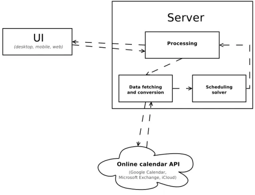
Figure 3.1: Diagram of monolithic server based web application

An example of how the algorithm along with the Data Fetching and Converting module can be used is presented in Figure 3.1. The relevant components and systems are distinguished on the diagram. The following process would be used to schedule a meeting in this scenario:

(17)

3.1. System overview 17

• The host uses theUI to create a meeting, which is sent to the server • Theservernotifies guests about the new meeting

• Guests authorize the application to access their online calendars through theUI

• The authorization details are used by the DFCto gather the guests’ events and convert them into the common format required by the scheduling solver

• The events, as well as the rest of the meeting parameters are passed to thesolver

• Thesolverresponds with its solution, which is passed to the processing layer • Theprocessing layernotifies the participants about the suggested meeting times In the likely event that some users of the system do not use any online calendar service, it would be straightforward to implement a simple UI widget for manual marking of events and only the DFC would need to be extended to accommodate this new data source. Then every user could take advantage of the system, regardless of how they keep their calendar.

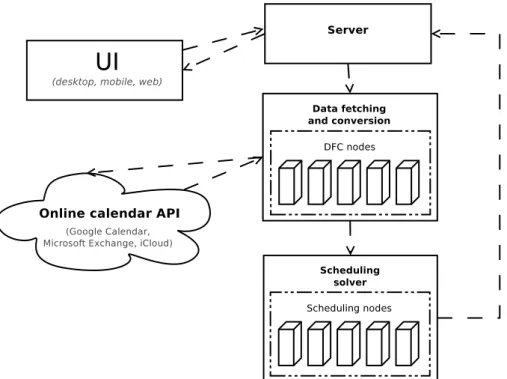
Figure 3.2: Diagram of a scheduling application based on a set of distributed services The scheduling solver may also be used as a standalone service if wrapped in a server which will handle communication with its consumers (other services). Figure 3.2 illus-trates an example architecture required for a standalone, scalable meeting scheduling application. The scheduling solver and DFC are now present as a separate components, which can be horizontally scaled as needed and can be placed e.g. behind a load bal-ancer. When utilising parallelism in meeting scheduling, it is important to consider the possibility of scheduling clashes. This problem stems from the fact that the library is designed to schedule one meeting at a time and operate only on a single snapshot of the event data. The difficulty of creating a complete parallel solution is compounded by

(18)

the fact that our library does not schedule meetings, but rather suggests the best times and it is up to the users to actually schedule the meeting. It is therefore not known immediately when a new event has been scheduled. This may lead to conflicts such as suggesting two meetings at the same time. If we assume, and this seems a rather reasonable assumption, that it is the user’s responsibility to resolve such conflicts, then the scheduling library can be easily parallelized. This is a trade-off that has to be made when looking to improve performance.

3.1.2

Multiple suggestions

Deciding on the best meeting time for a number of participants is a complex issue, as many factors have to be taken into account. While including preferences in the algorithm enables users to specify their idea of the suitability of possible options, it does not allow the system to schedule a meeting with 100% certainty that it is in fact the best option as judged by participants. The initial idea was therefore to design the algorithm in such a way that it can present a number of best solutions, in order to give a human controller the flexibility to choose the most suitable time. The methods for solving constraint satisfaction problems used, specifically the implementation of the Branch and Bound algorithm attempts to find the best solution as soon as possible and does this by discarding parts of the search space. Therefore, it does not allow the user to find multiple best solutions in one go, but only a single one. It is possible however, to return multiple solutions by running the search once for each required suggestion, adding constraints which exclude results obtained earlier. The disadvantage of this approach is its performance, as for n suggestions and T - the time taken by a single search, the procedure would taken∗T time to calculate all suggestions. In cases where the domain of the problem, that is the meeting window and number of participants, is small, the benefits are likely to outweigh the time disadvantage. However, on a larger scale, it is possible that it will not be feasible to suggest more than one meeting time. Most realistic situations result in the search space being manageably small, making multiple suggestion a possibility. In order to allow users to take advantage of their benefits, this feature has been implemented in the algorithm and can be set by the user for each problem separately.

3.2

Inputs and outputs

The following section describes the data representation and structure as well as the relationships between the data. The mechanisms of the scheduler will be made more clear in order to help the reader understand the implementation decisions made in the algorithm. The following are described below: events, preferences, calendars, meeting window, meeting length, the relationship between event and regular preferences, as well as the output of the algorithm.

(19)

3.2. Inputs and outputs 19

3.2.1

Inputs

The algorithm requires the following inputs in order to schedule a meeting: • List of calendars (one for each participant)

• Meeting window • Length of meeting

• Number of suggestions required

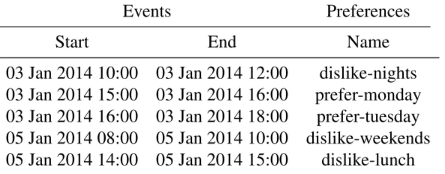
A calendar represents the schedule of a given user. It consists of a list of events and a list of preferences, which will be used to build a full image of the scheduling possibilities for that user. An event has only two properties: a start and an end. Both are dates with times, specifying an exact point in time when the event start or finishes, respectively. Preferences are functions, defined in the library, which take as input a time interval and return a number describing how much the given interval is preferred or disliked. This number, called thepreference value, is in the range from -5 (highly disliked) through 0 (neutral) to 5 (highly preferred). A set of such preference functions can precisely describe the preferences of a user in the selected meeting window. The values of individual preferences are added together, however if the sum is less than -5 or greater than 5, it is set to -5 and 5 respectively, so that it always fits in this range. This forbids creating unusually high or low preference values, which would unfairly increase a calendar’s importance. A number of general preferences are available to choose from in the library, along with constructors for creating more specific ones. Because of the wide variety of possible uses, the library does not discriminate certain times, e.g. through disallowing meetings at night. This can be handled better by the caller who can simply specify that every participant has a dummy event scheduled through the night, which would effectively prevent scheduling events during the night. Preference design is described in more detail in Section 3.5. Example preferences are:

• dislike-nights- dislike intervals which happen between 10pm and 6am • spread-events- dislike intervals which are close to scheduled events • clump-events- prefer intervals which are close to scheduled events • prefer-tuesday- prefer intervals which happen on Tuesdays

• dislike-lunch- dislike intervals which happen during lunchtime

In order to make it easier to visualize the structure of a calendar, example data is presented in Table 3.1.

Apart from a list of calendars, the scheduling library requires additional data in order to perform its task. The first of them is themeeting window, which has the same structure as an event, i.e. only a start time and an end time. The next one is the meeting length in minutes. It should be a multiple of 15, as the library divides the time into 15-minute intervals. It will be rounded to the nearest multiple of 15 internally, therefore it is recommended to use multiples of 15 in order to ensure that the meeting is scheduled as expected. The last input is the number of solutions required, which must be an integer

(20)

Events Preferences

Start End Name

03 Jan 2014 10:00 03 Jan 2014 12:00 dislike-nights 03 Jan 2014 15:00 03 Jan 2014 16:00 prefer-monday 03 Jan 2014 16:00 03 Jan 2014 18:00 prefer-tuesday 05 Jan 2014 08:00 05 Jan 2014 10:00 dislike-weekends 05 Jan 2014 14:00 05 Jan 2014 15:00 dislike-lunch

Table 3.1: Calendar structure with example data

greater than 0. It is important to note that, as discussed in Subsection 3.1.2, increasing the number of suggestions causes the performance to deteriorate proportionally. Table 3.2 shows an example of a complete set of input data for a meeting with 5 participants, withC1throughC5denoting user calendars, of the structure shown in Table 3.1.

Calendars Meeting window Length Suggestions

Start End

C1,C2,C3,C4,C5 03 Jan 2014 10:00 06 Jan 2014 19:00 60 5

Table 3.2: Structure of all inputs with example data

3.2.2

Outputs

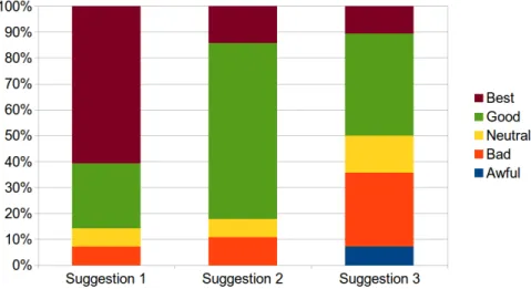
The algorithm outputs the requested number of best meeting times, all being fully inside the meeting window. It is important to note that, when using the suggest-soft

function, it will always return the given number of suggestions, even if there are no ”good” solutions. In extreme cases, such as when all participants are very busy, there may be no mutually free slots and the algorithm’s best suggestions will all require one or more users to reschedule. The suggest-hardfunction returns an empty list if there are no times when every participant is free. The suggestions are sorted in decreasing order of total preference. That is, the first suggestion is always the best, with each next being equal or worse. There is no guarantee of order between suggestions of equal preference. The solutions are annotated with additional information, which may help the user in differentiating between them. Each meeting suggestion consists of the following data:

• Start time • End time

• Total preference for this time

(21)

3.3. Cost function 21

The only situation when the algorithm will return less than the required number of suggestions is when there are fewer different meeting possibilities in the meeting win-dow. Remembering that the window is divided into 15 minute chunks, assume a 60 minute long meeting is to be scheduled in a very small meeting window of length 1.5 hours (e.g. between 1 May 4pm and 1 May 5:30pm). This window will be divided into 6 chunks. Each meeting slot takes up 4 chunks, allowing 6−(4−1) =3 distinct possibilities. In this situation, the algorithm will be able to output at most 3 solutions. Requesting more solutions will not cause an error, but only the 3 possible solutions will be returned. If the meeting window is even smaller, so that not even 1 meeting will fit, the algorithm returns an empty list.

The total preference value is a measure of how well the suggestion fits the participants’ schedules. This value corresponds to the preference score obtained by the constraint solver, but is normalized so that it is always in the range of 0 to 100. This is done present a clean interface to the users of the library and separate them from the algo-rithm’s internal representation of preference values. The individual preferences are similarly on a scale from -5 to 5, except when the suggestion clashes with a partici-pant’s schedule. In this case that person will have the number -100 as their preference. Note that a suggestion which borders on an event (e.g. starts exactly at the end of an event) is considered a clash, as the user will not have any time to make the meeting. The range from -5 to 5 is the same as the input range for preferences, which should make it easier to understand the preferences of each user for a given suggestion. Table 3.3 shows the structure of a possible scheduling output for the input data contained in Table 3.2.

Individual Preferences Total preference Start time End time U1 U2 U3 U4 U5

82 06 Jan 2014 16:00 06 Jan 2014 17:00 5 4 5 1 1

47 06 Jan 2014 13:00 06 Jan 2014 14:00 1 5 -2 -2 3 47 06 Jan 2014 08:00 06 Jan 2014 09:00 1 1 3 -1 -2 37 03 Jan 2014 16:00 03 Jan 2014 17:00 -3 0 0 -1 -2 37 03 Jan 2014 13:00 03 Jan 2014 14:00 -3 2 -2 5 -3

Table 3.3: Structure of the output, with example data

3.3

Cost function

An important design decision must be made with regard to the choice of the method by which the preferences of users are combined into a single value that can be used to rank different solutions. A higher preference indicates that the solution is better, so that the system will attempt to find a solution with the highest total preference possible. Formally: Assuming that for two solutionss₁ and s₂, s₁≺s₂ means that s₁ is worse thans2and given tuples(p1,s1)and(p2,s2)we have:

(22)

Thecost functionis defined to be the function which maps the preferences of the users to the total preference for each candidate solution. It has a large influence on the behaviour of the algorithm, as it decides which solution is optimal. However, there is a wide variety of candidates from which we can choose the cost function to be used in the algorithm. It is therefore important to consider what effect the candidates will have on the ranking of meeting suggestions, as well as what characteristics and behaviour is preferred for this particular problem.

The end goal of the algorithm is to find a meeting which will be most suitable for all participants. Ideally, the meeting would happen at the time which is the most preferred for each user. However, in reality it is highly unlikely that such a solution would be possible. Trade-offs must be made, leaving some participants less satisfied with the outcome. This gives rise to the question: how should the satisfaction of one human be compared to the satisfaction of another and how can values composed of distinct people’s preferences be compared to find a truly preferred outcome?

Modern utility theory deals with finding an answer to this and similar questions. A number of systems for interpersonal utility comparisons have been proposed, such as those by Edgeworth, Hausman and Harsanyi. However, these theories find little practical application in the problem at hand, due to the restricted knowledge present in the preferences as well as the criticisms to their practicality (see Binmore [11]). Therefore, in order to arrive at a function which yields the best results for the users, a number of possible alternatives will be described and compared.

One possibility is to use theutilitarian collective utility function, which is the sum of each user’s preferences for the given meeting time. This method in effect maximizes the average of users’ preferences and the trade-off between its constituents is linear: assuming preference values between 0 and 10, for two participants the intervals with preferences 9 and 1, 3 and 7, 5 and 5 are equally good. I conjecture that, in accordance with the law of diminishing marginal utility, the difference for an individual between two times with different preference values decreases as the values increase. Therefore, when analysing three such possible suggestions, the first certainly appears the worst, due to the fact that although it is a very good time for one, it is very unsuitable for the other participant. In this case the last suggestion, equally preferred by both partic-ipants, should be chosen, as no one is very much inconvenienced by this solution. The evaluation analysis in Subsection 5.2.2 shows that this hypothesis holds.

Trying to make sure that participants are inconvenienced as little as possible, the cost function could be set to be the minimum of all preference values, also called the egal-itarian collective utility function so that the algorithm will attempt to find a solution which has the highest minimum preference value. This method however, essentially takes into account only the minimum value and does not distinguish between different solutions with the same minimum values. This could be done by then reverting to a sum and comparing two sums, but there is a simpler way which meets the requirements set out earlier.

The idea is to use theNash collective utility function, that is the product of each user’s preferences, as the cost function. It will favour balanced solutions, discouraging so-lutions where one participant suffers for the benefit of another. Returning back to the

(23)

3.4. Use of Constraint Logic Programming 23

above example, for intervals with preferences 9 and 1, 3 and 7, 5 and 5, the products are 9, 21 and 25 respectively. The difference between the first and last solutions is significant, in agreement with the intuition that lowering one preference in order to increase another one leads to worse results. The negative aspect of the Nash function is that its results grow exponentially with the number of participants. While the lan-guage used can handle very large numbers, the solving library can only handle variable values that fit in the range of the Java int type. In order to be able to find meetings for large groups, when there are too many participants the egalitarian function is used. As described above, it also has the desired properties, but fails to distinguish between similar situations. Therefore the egalitarian function is used in the solver, with the Nash function being used to rank the suggestions returned by the solver. This allows the algorithm to find a number of suitable results and rank them according to the total preference of the group.

3.4

Use of Constraint Logic Programming

The search for an optimal solution with the given constraints is performed by a con-straint programming library, which implements the handling of concon-straints as well as performs the search according to a suitable algorithm. This library is CloCop ([1]), which is a Clojure wrapper around the Java constraint solver JaCoP ([5]). It is a fast and open source finite domain constraint solver, which supports a large variety of global and finite domain constraints.

The design of the algorithm was created in two stages: first based on hard constraints with preference sorting applied outside of the solver, then using that framework with soft constraints, to integrate the preferences into the problem solved by the CSP library. The initial version specifies hard constraints on the meeting time with regard to the participants’ events. The meeting must not overlap any event in order to be regarded as a possible solution. The solver then searches for all possible meeting times, such that every member of the group can participate in the meeting. The possibilities returned by the solver are all equal, as they do not have preference values assigned to them yet. This is managed by a separate routine, which calculates the cost function using all the users’ preferences and sorts the events according to their cost. This allows the system to return multiple suggested solutions along with their cost and let the user make a more informed decision based on other factors.

The soft constraint design can be thought of as an evolution of the first phase, as it uses the same flow of information and conversion of real-world data to internal representa-tions, but can find solutions even when no single time window is free for all attendees. The events and preferences are both represented by soft constraints, with events be-ing conceptually analogous to highly disliked intervals. The solver computes the cost function as a variable and tries to minimize it during the search. The solution returned by the solver is then already the current best possible meeting time, so that there is no need to process the results, except for conversion back to a format understandable by the host system. As a side note, it should be mentioned that representing events by preference values enables the algorithm to be more flexible when accounting for them.

(24)

As an example, the system could be extended to apply machine learning techniques to event data (such as its name, place and time) to predict the importance of events and difficulty of rescheduling events. Events which are deemed to be less important or easy to reschedule, could have a lower cost, while important events would be assigned a much higher cost. The algorithm would then be more likely to schedule meetings overlapping unimportant events if that fits the group’s preferences better. On the other hand, it would be less likely that a suggestion overlaps a user’s important meeting, such as a wedding, and unimportant meetings would be ”sacrificed” first.

The performance of the algorithm depends highly on choosing suitable values for the preferences representing events. These values have to be chosen in relation to the domain of user preference values. The range of possible values can be narrowed down by considering the desired outcome of the scheduling algorithm, then further fine tuned using empirical methods. An initial observation is that, lacking knowledge about the importance of events, the algorithm should strive to schedule meetings that collide with as few participant events as possible.

3.5

Preference design

Preferences used in the algorithm perform two related functions: checking whether a given time interval fits the preference, and providing a numerical value for it if it does. A simplistic approach would be to design preferences as tuples of the form: < f,n>, where f is a function that takes a time interval and returns a boolean andn

is the preference score, or cost, of that preference. The algorithm would then check whether the function returns true, and assign n as the cost of the interval. However though it makes creating preferences very easy, this approach causes them to be rather inflexible. For example it makes it very difficult to implementsmooth preferences, that is ones which can be partially satisfied, making the cost a function of the satisfaction of the preference. In order to allow such preferences to be implemented, they should be designed as modifiable functions. This method has been utilised in this work. Each preference has a corresponding constructor, which takes some arguments and returns the preference function of the type described above. The constructor arguments de-pend on the preference and can range from a constant to a function which takes some arguments and returns an integer. The preference function now takes a time interval and the list of events, and returns an integer describing the cost of that time interval. This allows a wide variety of flexible preferences to be created, even with relatively complex behaviours and the ability to describe preferences in terms of the whole of the user’s schedule, rather than just the time. One example of taking advantage of this ability is theclump-eventspreference. It is used when a user prefers to have their events close together, as it gives higher preference values to intervals which are close to already scheduled events. Additional preference functions can be added to the system by simply implementing new functions with the required signature.

Some existing solutions, such as Doodle ([2]) and ScheduleOnce ([8]) do not incorpo-rate preferences, leaving it to the user to decide which slot is best. Timebridge ([9]) only allows users to specify one slot as a ”Best” slot. The preference system designed

(25)

3.5. Preference design 25

in this work is much more flexible, enabling users to utilize patterns in their sched-ules to specify multiple preferred or disliked slots simultaneously, such as disliking lunchtime or clumping events (as described above). The preferences are also compos-able, e.g. disliking Mondays and lunchtime yields a strong dislike for meeting during lunch on Mondays. This also has a positive impact on the conciseness of this system, as it automatically orders meeting times using the preference scores.

(26)

(27)

Chapter 4

Implementation

The algorithm is implemented as a library to be used in a larger system. It expects the host to pass data to it in a valid, recognized format independent of the source of the data. The system itself must therefore be able to convert users’ events and preferences from the structures it obtains them in to those used by the algorithm. As suggested in Subsection 3.1.1 a separate module can be used to this end. It has not been made part of the library and was not in the scope of the project, because of the large amount and variety of possible representations used in a system. Such a conversion module could be reusable in other domains, if it were able to convert from a number popular source formats. Sources such as Google Calendar, Apple Calendar or Microsoft Exchange would certainly be used often, however many systems would still have to implement conversion mechanisms for their own data sources. In this chapter, we will describe some of the more important details of the internal implementation of the scheduling algorithm and its use of the constraint solving library.

4.1

Description processing steps

This section describes the entire process of computing a meeting suggestion, step by step.

1. The algorithm can be called using the functionsuggest-soft, which receives in-puts of the form described in Section 3.2.1. These are:

• An array of calendars, one for each participant, with each calendar being a hash-map containing a list of events and a list of preferences

• The meeting window - a hash-map specifying the first possible start time of the meeting and its last possible end time

• Length of the meeting in minutes, which should be a multiple of 15 (the time resolution used by the algorithm) and will be rounded to the nearest multiple of 15 if it is not

(28)

• Number of solutions required - as described in Subsection 3.2.2, the al-gorithm will always return this number of solutions, except if the meeting window is not large enough

2. An array of preference values is created from the calendar, for each user. Each element is the user’s preference for a meeting starting at that time. The time of each element is specified by its index, with the first being the start of the meeting window and each next element being 15 minutes later than the previous one. The last element’s time is such that the meeting starting at this time will finish before the end of the meeting window. More formally, thenthelement contains the preference of a suggestion starting atwindowStart+ (n−1)∗15minutesand ending atwindowStart+ (n−1)∗15minutes+meetingLength. The preference values are normalized to the range used internally, described in Section 4.2. Note that when a time clashes with an event (by overlapping or bordering with it) it gets a preference value of 1 in the internal scale. This is its final value, which is not modified by preferences.

3. In order to represent the meeting window (the space of possible meeting start times) using a finite domain variable, the window is converted into integer form. The start always has the value 0. Each following number represent a time 15 minutes later than the last. The end has a value which is equal to the number of full 15 minute intervals in the meeting window. As an example, for a meeting window with start: 15/05/2013 2pm and end: 17/05/2013 10am, the integer rep-resentation has start: 0 and end: 176. The value 16 would correspond to the date 15/05/2013 6pm. Note that this conversion process is the same as the one used when creating the preference arrays, which means that the integer representation can be used as an index into the preference array.

4. For every suggestion required, CSP variables are created, constraints are set on them and the CloCoP library is used to solve the CSP. Each iteration is provided with the solutions from the previous iteration, which have to be excluded from the search space.

(a) Astart variable, which represents the start time of the meeting is created. Its domain is defined using the integer representation of the meeting win-dow. The minimum of the domain is the start of the meeting window, while its maximum is the integer describing the last possible start time. If there are any solutions that should be excluded, hard constraints are put on the variable to ensure that it will not be the same as any of the previous solu-tions.

(b) A person-pref variable is created for each participant. Its domain is the same as the domain of thestart variable. It represents the person’s prefer-ence of the current meeting time. Its value is the element of the person’s preference array at index start (the value of the start variable is used to index into the preference array).

(c) A total-pref variable is created, which represents to the total preference of the given meeting time. Its value is the combination of the individual

(29)

4.2. Preference values 29

person-pref variables using the collective utility function. Using the Nash product during solving may result in integer overflows for groups of more than 5 participants. The egalitarian function is used then, with the Nash product being used for sorting the results.

(d) The created variables and constraints are passed to the solver library (Clo-CoP), indicating that the value of thetotal-pref variable should be maxi-mized1. CloCoP solves the given CSP and returns the values of all variables for the best meeting time found. The resulting suggestion is added to the end of the array of suggestions. This results in all the suggestions ending up in order of decreasing total preference if the Nash product has been used. 5. If the egalitarian function was used, the Nash product of each suggestion is

cal-culated and assigned as the total preference value. The preferences are then sorted in decreasing order of total preference.

6. The values of the preferences (both individual and total) in all the suggestions are converted to the scales used for output, as described in Subsections 3.2.1 and 3.2.2.

7. The results still have the meeting start found by the solver in integer representa-tion. It is now converted into a DateTime object and its appropriate end time is added to the suggestion, also as a DateTime. This is the final step, as the results are now in the form specified in Subsection 3.2.2, so they are returned.

When calling thesuggest-hard function, the process is similar, with the exception of the CSP variables and constraints set on the problem. Here constraints are set on the

startvariable to disallow the meeting to overlap with an event.

4.2

Preference values

Internally both preferences and events are described in the same way: as numbers which describe how much the user would like to meet at this time. There must be a large difference between the value of a user preference (e.g. prefer-tuesday) and an event preference, in order to ensure that free slots are chosen before scheduled slots. Because of the fact that a busy slot is simply one which is very disliked, the ratio between the values attached to the user preferences and those attached to the events is an important influence on the characteristics of the algorithm’s solutions. This ratio is not configurable by the user, but was chosen by the author with regard to the characteristics of the problem domain. Internally, when using soft constraints, the algorithm treats events as very strong preferences, because they need not be respected - the library allows solutions which clash with a user’s scheduled events. However, it is the assumption of the author that such suggestions should be avoided if at all possible (this assumption is tested in Section 5.2.1). Therefore the ”weight” of an event is set so that slots which are disliked by everyone are rated as better than ones that are liked,

1_{To be specific, the solver minimizes the negation of total-pref, which is equivalent to maximizing}

(30)

but cause a clash in someone’s calendar. It is also desired that slots that are unbalanced (i.e. highly disliked by some user, but highly liked by others) are rated as worse than more balanced ones (i.e. neutrally liked all around). In order to help balanced solutions have a higher rank, the neutral score should not be in the centre between the worst and best preferences, but should be moved closer towards the best score. This will cause neutral slots to have a higher score than they normally would. The criteria are met by setting the range of preferences to that shown in Table 4.1.

Event Worst Neutral Best

1 20 35 40

Table 4.1: Internal preference values

4.3

Constraint satisfaction implementation

The CSP solver library used in the implementation specifies finite domain variables, that is, it solves problem defined on integers. The dates and preferences describing the meeting scheduling task must therefore be converted into an integer-based representa-tion. Time is divided into equal-sized chunks, calledtime-resolution units, according to the time-resolution of the algorithm, so that they can be indexed easily. Every chunk is converted into a natural number, with 0 being the first possible start time (the start of the meeting window) and increasing by 1 for every unit of time-resolution (e.g. 15 minutes), until the end of the meeting window. As a result, each possible start time is uniquely identifiable by an integer, which allows a variable to be defined on the integer range.

The events and preferences are combined into a preference array with one entry for each value in the variable’s domain. Each entry contains a single participant’s cost of scheduling a meeting at that time. Each participant has their own preference array. Using thenthpiping function, the solver can create a CSP variable which will be equal to one of the values in an array. The array and the index into the array are given as arguments to the function. The array can contain constants or variables. The index is specified to be the value of a variable. In the algorithm, we use the preference array and the start time variable as the index. The result of the piping function is then a variable which holds the user’s cost at the currently evaluated time slot.

The individual costs are combined together using the collective utility function. The solver uses the Branch and Bound algorithm to find the largest value of the function and its associated start time. It returns this time (in its integer representation), as well as the individual preferences and the value of the cost function.

(31)

4.4. Data-structure preparation 31

4.4

Data-structure preparation

The constraint satisfaction library used as the solver is a multi-purpose tool designed to be used in a variety of domains, to solve a large range of problems. The data passed to the algorithm must therefore be converted into a problem description that fits the framework of the solver. As described above, the problem data is represented using integers. Possible start times are always between 0 and N, where N is the number of time-resolution units between the start and end of the meeting window. The preference arrays are constructed by using either the sum of the values of preference functions or the event cost (if the interval overlaps with an event) for each time interval between the start and end of the meeting window. The index of the array represents a candidate start time, while the value at this index represents its cost for the given participant. Due to a sign error in the implementation of the solver library, the start times had to be adjusted to fit the array indices, as it acts as if the array starting index was 2, rather than 0. These start times must then be normalized back to their initial values after finding a solution.

4.5

Library consumer interface

The use of the library should be influenced as little as possible by the internal represen-tation of data structures and preferences. Presenting a clean, fixed interface will allow the users of the library to continue to use it in the same way even after changes to the internal mechanisms are made. This allows the developers the freedom to improve the design and implementation of the library without disrupting its users.

A clean interface is maintained by expecting and returning data in a specified, uniform format to and from the user. Firstly, the users preferences are expected to be given as an integer in the range -5 (disliked) to 5 (preferred), with 0 being neutral. The individual preferences for the suggested timeslots will also be returned in this range, for ease of comparison and understanding their values. The total preference for a timeslot will be given in the range from 0 to 100, with 0 being the worst possible scheduling and 100, the best. Such a fixed suggestion score is designed to help users of the library understand how well each slot is liked by the group and whether all are good fits or not. Another important conversion must be made in order to allow the users to understand the library’s suggestions and let the constraint solver do its work. That is, as described above, the conversion of dates to an integer representation for constraint solving and then converting the integer suggestion back to a date on output.

(32)

(33)

Chapter 5

Evaluation

In order to judge whether the algorithm may help simplify complex procedures in-volved in scheduling meetings for groups of individuals, its suggestions must be tested by users to help decide whether they could be satisfactory in real-life conditions. To achieve this goal, an evaluation procedure must be specified and carried out. The data gathered from this measurement should give the opportunity to identify both strengths and weaknesses of the system, so that they can be addressed and the algorithm can be improved.

5.1

Evaluation method

Users will be presented with multiple scenarios, each of them a situation when a num-ber of people want to schedule a meeting together. The experiment should ideally be completely repeatable, so it would be best if the scenarios were predetermined by the author, rather than dependent on the particular time or subject of the experiment. Syn-thetic scenarios, consisting of calendars with events and preferences will be created beforehand. Using the same sets of scenarios for all experiment participants will im-prove the consistency of the results and imim-prove the repeatability of the evaluation. When crafting synthetic data, it is important to address the issue of representativeness of the created data. The scenarios should be varied enough to test as many different types of situations as possible out of the many that can arise in real-world usage of the algorithm.

Experiment participants will be asked to rate the algorithm’s solution as well as sug-gest a different one if they consider it to be better suited to the scenario. This will provide information about the suitability of the answers returned by the algorithm and help show what could be changed or improved in the implementation. This could be achieved by gathering participants into groups, with each receiving a persona in the scenario and then having them negotiate with each other to agree on the best time to schedule a meeting and on the rating of the algorithm’s solution. The advantage of this method is that it imitates the negotiation process that happens when meetings are

(34)

scheduled in real life, which in theory could result in more realistic outcomes. How-ever, the variability and significance of human group behaviour dynamics could have a strong influence on the results. This would be an added undesirable variable in the ex-periment, decreasing its quality. An example of this effect can be a situation in which a single person in the group has better persuasive skills than the others and is able to get them to agree on a time that is more suitable for that one person, but less suitable for the others. The software is not only unable to predict the negotiation strength of participants, it aims to ensure that its suggestions are as good as possible for all the participants. The experiment would be made more reliable if that dynamic behaviour can be avoided completely, or at least diminished.

This behaviour can be avoided by performing the experiment with individuals rather than groups. In this case the subject is asked to look at the calendars in the scenario, rate the algorithm’s solution and describe a better one if the algorithm’s suggestion is lacking in their opinion.1 The order of rating the suggestions and looking for a better one is important for the results. If the algorithm’s suggestion were presented after asking the subject to name the best meeting time, there is a risk that their solution may not be as good, yet they would feel pressure to justify it and rationalize their choice. This would cause the algorithm to be rated lower than it is reality, hurting the reliability of the results. Therefore, the algorithm’s suggestion should be shown first, so that there is no pressure for the subject to agree or disagree with it and they are likely to be more objective. Performing the experiment with individuals does make the assumption that the subject will be able to take into account the preferences of the personas and make the decision about which time is best for the group and that a balanced2group would also find this solution satisfactory. An additional advantage of using individuals is that the experiment can gather a larger amount of data-points using the same number of subjects. This means finer and more reliable conclusions can be drawn from it.

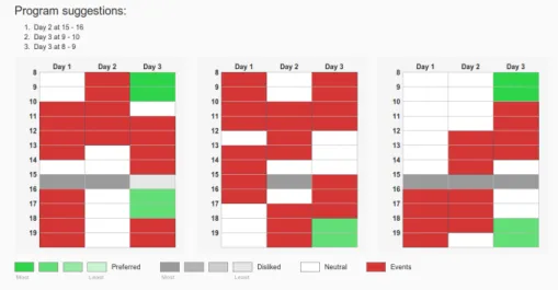
The evaluation was performed according to the rules outlined above, by creating a web application which presented the scenarios and gathered users’ responses. The scenarios were represented by a visualisation of a calendar with events and preferences marked as coloured boxes. Initially the events were marked as blue, in similarity to the default colour of Google Calendar events. The preferences were marked by a range of colours from red (disliked), through white (neutral) to green (preferred). Before launching the evaluation website, a beta test of the survey was performed. Participants were invited to complete the survey in person, having direct contact with the author. They were encouraged to discuss the survey and were asked a set of questions and tasks regarding their understanding and behaviour, including:

• Do you feel the survey instructions are clear?

• Explain, in your own words, what is expected of you

• Could you explain why you have chosen to give this suggestion this rating? • Describe the schedule of Person 1. When are they busy, which times do they like

1_{The calendars should all be presented as other people’s in order to avoid bias towards a particular}

calendar.

(35)

5.1. Evaluation method 35

and dislike?

The beta test revealed a number of flaws in the survey, which allowed it to be improved before being shared with a larger group of respondents. The first issue was the constant order of algorithm suggestions, which were shown from best to worst. This, combined with the fact that evaluating the calendars required attention and thought, caused lazi-ness in testers. After agreeing a number of times with the suggestions presented, they started paying less attention to the calendars and automatically rated suggestion in the same way. This would decrease the reliability of the results. In order to fix this, the suggestions were changed to show up in random order, thereby causing subject to need to evaluate the calendars correctly to determine which suggestion is best. Secondly, some testers, who used a different computer to perform the tests, noted that it is dif-ficult to see the colours that describe users preferences, which prompted them to be changed to more saturated versions. Thirdly, it turned out that the choice of red colour for disliked timeslots and blue colour for events confused participants, who thought the red meant b