C
ENTRE FOR
D
YNAMIC
M
ACROECONOMIC
A
NALYSIS
C
ONFERENCE
P
APERS
2009
CDMC09/02
The Interest Rate — Exchange Rate
Nexus: Exchange Rate Regimes
and Policy Equilibria
*
Christoph Himmels
†University of Exeter
Tatiana Kirsanova
‡
University of Exeter
AUGUST
28, 2009
A
BSTRACTWe study a credible Markov-perfect monetary policy in an open New
Keynesian economy with incomplete finacial markets. We demonstrate the
existence of two discretionary equilibria. Following a shock the economy can
be stabilised either 'quickly' or 'slow', both dynamic paths satisfy conditions
of optimality and time-consistency. The model can help us to understand
sudden change of the interest rate and exchange rate volatility in
'tranquil' and 'volatile' regimes even under a fully credible 'soft peg' of the
nominal exchange rate in developing countries.
JEL:
E31, E52, E58, E61, C61, F4
Keywords:
Small
Open
Economy,
Incomplete
Financial
Markets,
Discretionary Monetary Policy, Multiple Equilibria.
*Preliminary and incomplete. Please do not quote without consulting the authors first.
1
Introduction
Fixing nominal exchange rates is frequently justified as a way to avoid excessive variability of economic variables, in particular in developing countries. The idea behind an exchange rate peg is that it will increase trade directly through lower uncertainty and smaller adjustment costs, and indirectly through its effect on the allocation of resources and government policies (see Côte (1994)). It may also encourage investment into long-term projects due to lower exchange rate risk/ transaction costs and therefore has a positive economic impact (see Prasad et al. (2003)). Being prone to speculative attacks hard pegs became less popular, especially after the Asian crisis of 1997. However, recent evidence suggests that monetary authorities in many developing countries still see nominal exchange rate targeting as their priority, despite that they officially claim to have floating regimes.1 Developing and emerging countries like Indonesia, Malaysia,
Thailand, South Korea, Turkey, Russia adopted de jure flexible exchange rate regimes, but de facto the exchange rate remained one of the most important if not the only target of their monetary policy.2 Reinhart and Rogoff (2004) report that a crawling peg was the most common
type of exchange rate arrangement in the Asian emerging countries between 1990 and 2001. Despite the post-1997 decade was relatively tranquil in developing and emerging countries3,
the exchange rate volatility under these ‘soft pegs’ varied over time. There is a number of studies that document difficulties in explaining these sudden changes in ‘regimes’ with higher or lower volatilities.4 Theoretical explanations for these different regimes include non-rational behaviour,
non-linear decisions, heterogeneity of agents like the presence of ‘noise traders’ and so on (see Jeanne and Rose (2002) for an important example).
The main aim of this paper is to present a much simpler model that can help to understand some of these empirical facts. We claim that the wayhow monetary policy is conducted can be re-sponsible for the existence of time periods with large difference in the volatility of macroeconomic variables. We employ a simple linear stochastic model that has become the workhorse model in monetary economics and abstract from many features that may characterise many developing or emerging countries, e.g. capital control or incomplete exchange rate pass-through. However, we account for incomplete financial markets and study a discretionary monetary policymaker which uses the interest rate as its instrument. The assumption of a discretionary policymaker seems realistic as policy commitments are practically impossible in developing countries. This set up gives rise to multiple policy equilibria under different exchange rate targeting regimes. We show that under fully credible discretionary monetary policy and rational expectations there exist two equilibria that are associated with different speeds of adjustment towards the steady state and therefore with different volatilities of all macroeconomic variables.
Discretionary policy is time-consistent. A potential drawback of the time consistency con-1See e.g Levy-Yeyati and Sturzenegger (2005) and Calvo and Reinhart (2002).
2See Rahmatsyah et al. (2002) for Thailand, Das (2003) for Indonesia, Malaysia, Thailand and Korea, Doganlar (2002) for Turkey, Korea, Malaysia, Indonesia and Pakistan, and Arize et al. (2000) for 13 developing countries.
3We do not take into account the recent financial crisis.
4See e.g. Engel and Hamilton (1990), Clarida et al. (2003) or Chen (2006) who apply Markov-switching models to explain these changes. These models have also been employed to describe exchange rate behaviour in floating regimes. However, their succes is still a matter of current debate see e.g. again Clarida et al. (2003) and Engel et al. (2007).
straint is the possibility of multiple equilibria.5 Under time consistency, the policymaker takes
current and future economic conditions into account, but can only commit to current behavior. Economic conditions are affected by the response of the rational private sector and any response is based on a forecast of future economic conditions. As a consequence multiple equilibria may arise: Future policies respond to a state that is at least partly determined by forecasts of that policy. Different sets of beliefs about the future policy generate different future courses for policy to follow. Therefore, if the economy is hidden by a shock, it can follow one of several adjustment paths or regimes. The volatility along these paths is different. In presence of the several equilib-ria, coordination failure happens: the private sector can choose any of them. A sunspot decides which one will realise.
We demonstrate how the existence of strategic complementarities in our model generates mul-tiplicity of equilibria.6 Under conventional inflation targeting, following an interest rate increase,
the effect of consumption on the terms of trade reinforces the effect of the interest rate on the terms of trade. Thus we have a strategic complementarity between consumption and the terms of trade in their effect on marginal cost, which are crucial for the control of inflation. The result-ing two equilibria can be classified as ‘dry/patient’ and ‘wet/impatient’, based on the observed strength of interest rate responses. Then we look at a policymaker who introduces an additional positive weight in its policy objective that punishes the volatility of the nominal exchange rate (provided that the anchor country ensures price stability). In this case the ‘wet/impatient’ equi-librium becomes non-existent, while another equiequi-librium with higher social losses arises. When the weight on the exchange rate target completely dominates other terms in the objective of the policymaker (‘currency peg’), the policymaker is able to stabilise the exchange rate completely if the private sector expects the stable nominal exchange rate in one equilibrium. However, there is another equilibrium: if there is a common belief that the nominal exchange rate is going to depreciate/appreciate in the future — non-zero exchange rate volatility is allowed by the policy-maker’s objectives — it becomes optimal for a policymaker to validate these beliefs and generate the forecasted depreciation/appreciation. This is line with empirical work by Engel et al. (2007) who find that short-run movements in exchange rates are primarily determined by changes in expectations. Therefore the economy may be trapped in the worst equilibrium with high volatil-ity in all economic variables. If the penalty on exchange rate volatilvolatil-ity in the policymaker’s loss function is small relatively to conventional weights on inflation stabilisation, the resulting policy can improve the worst equilibrium only marginally, while the policy is always damaging for the best equilibrium. We argue that in our framework a ‘soft peg’ is, generally speaking, undesirable. The paper is organized as follows. The next section outlines the model. Section 3 discusses the two policy equilibria for two regimes, inflation targeting and nominal exchange rate targeting. Section 4 concludes.
5See King and Wolman (2004) for a non-linear model and Blake and Kirsanova (2008) for a general discussion of multiplicity in LQ RE models under discretion.
6See Cooper and John (1988) and King and Wolman (2004) for a discussion about the relationship between mulitiplicity and complementarity.
2
Model
The framework is relatively standard and builds heavily on the small open economy model in-troduced by Galí and Monacelli (2005), but we allow for a non zero current-account balance by including incomplete financial markets following a framework proposed by Benigno (2001).7
Since our country is small its economic performance and its domestic policy decisions do not have any impact on the rest of the world. Both economies are populated by a continuum of infinity-living households, which consume two goods. One is produced domestically and the other good is imported from the foreign country. The law of one price holds, but deviations from purchasing power parity (PPP) arise due to the existence of home bias in consumption. Production takes place in two stages. First, there is a continuum of intermediate goods firms, which produce a differentiated input. In the second stage final goods producers combine these inputs into output and sell them to households in both countries. Monopolistic competition and sticky prices are introduced to get a meaningful role for policy.
2.1
Households
Both economies, home (H) and foreign (F), consist of a continuum of infinity-living households and share identical preferences and technology. We assume that every household seeks to maximize
E0 ∞ t=0 βt (1−χ)C 1−σ t 1−σ +χGt− Nt1+ϕ 1 +ϕ (1) where Ct denotes private consumption and Nt hours of labour, while Gt is an index of public
consumption. β is the subjective discount rate and E0 is the actuarial expectation at timet= 0.
Furthermoreχ∈[0,1]is the weight attached to public consumption and1/ϕmeasures the Frisch-elasticity of labour supply. In more detailCt is a composite consumption index defined by
Ct≡ (1−α)1η(CH,t) η−1 η +α 1 η(CF,t) η−1 η η η−1
Parameter η > 0 denotes the elasticity of substitution between domestic and foreign produced goods from the viewpoint of the domestic consumer. CH,tand CF,tare the Dixit-Stiglitz indexes
of consumption of domestic and foreign goods given by the CES functions
CH,t= 1 0 CH,t(j) ǫ−1 ǫ dj ǫ ǫ−1 ; CF,t= 1 0 CF,t(j) ǫ−1 ǫ dj ǫ ǫ−1
wherej∈[0,1]denotes the good variety andǫ >1is the elasticity of substitution between varieties of goods produced within a given country. Parameterα∈[0,1]is the weight of imported goods 7In a very similar model De Paoli (2009b) analyzes the welfare effects of incomplete financial markets under Ramsey (precommitment) policy and Erceg et al. (2007) investigate how current account dynamics affects the transmission mechanism of domestic shocks.
in private home consumption and is inversely related to the degree of home bias in preferences. Another interpretation forαis as a natural index of openness.
The nominal intertemporal budget constraint at timetfor householdibelonging to country H is given by 1 0 [PH,t(j)CH,ti (j) +PF,t(j)CF,ti (j)]dj+Et Di H,t+1 1 +it +Et EtDiF,t+1 (1 +i∗ t)φ EtDF,t +1 Pt ≤Di H,t+EtDiF,t+ (1−τt) Wi tNti+ Πit +PH,tTti (2)
wherePH,t(j) is the price of domestic goodj and PF,t(j)denotes the price of variety j imported
from countryF, where the latter is expressed in domestic currency. Wti is the nominal wage and Ti
t denotes lump-sum taxes/transfers. τ denotes a country specific tax on nominal income andEt
is the nominal exchange rate, given as the price of one of unit foreign currency in terms of home currency. We assume that the households share the revenues of owning firms in equal proportion. Following Woodford (2003a) we consider a cashless economy. Therefore the only explicit role played by money is to serve as a unit of account.
We introduce incomplete financial markets by applying a framework proposed by Benigno
(2001).8 Households of country H can trade in two nominal one-period, risk-free bonds. One
bond is denominated in home currency, the other in foreign currency; but home currency denom-inated bonds are only traded domestically. So only the foreign bond is traded internationally. Furthermore, households belonging to countryHhave to pay an intermediation cost, if they want
to trade in the foreign bond.9 Let D
H,t and DF,t denote the holdings in the home and foreign
bond of all households belonging to countryH. Let a ”∗” denote foreign country variables. The
gross nominal interest rates of the home and foreign bond are given by 1 +i and 1 +i∗,
respec-tively. As mentioned above households have to pay a price to trade in the international market. These costs are determined by the functionφ(·). Functionφ(·)depends on the real holdings of the foreign assets in the entire economy, and therefore is taken as given by the domestic households. If a household belongs to a country which is in a "borrowing position" (DF,t+1 < 0), it will be
charged with a premium on the foreign interest rate and if the household belongs to a country which is in a ‘lending position’ (DF,t+1 > 0), it receives a rate of return lower than the foreign
interest rate. Along with Benigno (2001) we need the following restrictions onφ(·): φ(0) = 1and
φ(·) is 1 only ifDF,t= 0. Furthermoreφ(·) has to be a differentiable, decreasing function in the
neighborhood of zero.
The intermediation profits K are defined analogous to Benigno (2001)
K= D ∗ F,t+1 Pt∗(1 +i∗t) 1 φEtD ∗ F,t+1 P∗ t −1 >0
Pt∗Ct∗+
DF,t∗ +1
(1 +i∗t)
=DF,t∗ + (1−τ∗t) (Wt∗Nt∗+ Π∗t) +PF,tTt∗+K.
The demand for good j produced in a given country can be written as
CH,t(j) = P H,t(j) PH,t −ǫ CH,t; CF,t(j) = P F,t(j) PF,t −ǫ CF,t
for allj∈[0,1], wherePH,t=
1 0 PH,t(j)1− ǫdj 1 1−ǫ andPF,t= 1 0 PF,t(j)1− ǫdj 1 1−ǫ
are the price indexes for domestic and imported goods, whereby the latter is expressed in domestic currency.
Finally, the optimal condition of expenditures between domestic and imported goods is given by CH,t= (1−α) PH,t Pt −η Ct; CF,t=α PF,t Pt −η Ct wherePt= (1−α)PH,t1−η+αPF,t1−η 1 1−η
Ptis the consumer price index (CPI) in countryH. Note
that if the economy is closed, α = 0, the CPI equals domestic prices. Correspondingly we can
write total consumption expenditures by domestic households asPtCt=PH,tCH,t+PF,tCF,t. The
aggregated budget constraint can therefore be rewritten as
PtCt+Et Dt+1 1 +it +Et EtD∗t+1 (1 +i∗ t)φ EtD∗ t+1 Pt =Dt+EtD ∗ t+(1−τt) (WtNt+ Πt)+PH,tTt. (3)
Maximizing (1) with respect to (3) yields the following FOCs:
β Ct Ct+1 −σ Pt Pt+1 = 1 1 +it (4) β Ct Ct+1 −σ Pt Pt+1 Et+1 Et = 1 (1 +i∗ t)φ EtD∗ t+1 Pt (5) CtσN φ t = (1−χ) Wt Pt (6) Et EtD∗t+1 (1 +i∗ t)φ EtD∗ t+1 Pt = EtD ∗ t +PH,t(Yt−GH,t)−PtCt (7)
Equation (4) is the standard Euler equation and determines the consumption smoothing behaviour of the households. Equation (5) is the Euler equation derived from the optimal choice of the foreign bond. Equation (6) is the standard labour supply condition. It determines the quantity of labor supplied as a function of real wage, given the marginal utility of consumption.
Finally, equation (7) is the aggregate budget constraint, which is obtained by aggregating the budget constraints of the households together with the government budget constraint (defined below). To derive this equation we also assume that output is distributed over wage and profits
WtNt+ Πt=PH,tYt.
A similar Euler equation holds for country F:10 β C∗ t Ct∗+1 −σ P∗ t Pt∗+1 = 1 1 +i∗t .
In contrast to the complete market case the monotonic relationship linking consumption with world consumption and ToT/ real exchange rate (see e.g. Galí and Monacelli (2005)) breaks down. The incomplete financial market framework generates deviations from the uncovered interest parity (UIP). Combining (4) and (5) yields the optimal portfolio choice of the households of
countryH (1 +it) = (1 +i∗t)φ(dt) Et+1 Et , (8)
where we simplified dt = EtDPtF,t+1. φ(dt) can also be interpreted as a risk premium term on the
exchange rate.11 If the economy is a net debtor, the domestic interest rate is above the foreign
interest rate and if the economy is a net creditor the domestic interest rate is below the foreign interest rate. Therefore movements in the net foreign asset positions affect the interest differential between the two countries.
Combining (5) with the Euler equation of the foreign country (8) yields the international risk sharing condition Et Ct+1 Ct −σ Pt Pt+1φ(dt) =Et C∗ t+1 C∗ t −σ Pt∗ P∗ t+1 Et Et+1. (9) Note that ifdt≡0thenφ(dt) = 1and the above equation simplifies to the standard international
risk sharing relationship which is obtained in a complete securities markets setting (see e.g. Galí and Monacelli (2005)).
2.2
Price and Exchange Rate Identities
The terms of trade are defined as the price of foreign goods relative to the price of goods produced
in countryH and given by
St≡ PF,t PH,t
Note that in this framework the PPP does not hold in the short run, because of the presence of home bias in consumption. However, PPP holds in a symmetric steady statePH =PF. Following
PF,t. This results from the definition of the rest of the world as closed economy, implying that
countryH goods production is a negligible fraction of the world´s consumption basket. Hence it
follows π∗t =πF,t for all t,whereπt= PtPt−1.
Under the assumption of free-trade in all goods the law of one price holds for all individual goods at all times and implies
PF,t(j) =EtPF,t∗ (j),
for all j ∈ [0,1]. Et is the nominal exchange rate and PF,T∗ (j) is the price of a foreign good
expressed in foreign currency. Aggregating across all goods implies
PF,t=EtPF,t∗ .
The real exchange rate — the ratio of CPI inflations, expressed in domestic currency — is defined as Qt= EtPt∗ Pt . (10)
2.3
Government
The government only provides goods and services which are produced in the domestic country. The public good aggregate of countryH is given by
GH,t= 1 0 G ǫ−1 ǫ H,t(j)dj ǫ ǫ−1 , ǫ >1
where GH,t(j) is the quantity of domestic good j purchased by the government. The demand
schedule of government spending is also similar to the consumption case and given by
GH,t(j) = P H,t(j) Pt −ǫ GH,t.
The government budget constraint in the home economy is given by
Et Dt+1 1 +it =Dt+PH,t(Gt+Tt)−τ PH,tYt, (11)
where τ is a tax on the nominal income of the domestic households and GH,t is government
spending, whereby both are exogenous and financed by lump-sum taxes/ transfers Tt.
2.4
Firms
2.4.1 Technology
There is a continuum of monopolistic competitive firmsj∈[0,1]in both countries and each firm produces a differentiated good with a linear technology, represented by the production function
where At is a exogenous, country-specific technology shock. The demand curve for each firm is given by YH,t(j) = PH,t(j) PH,t −ǫ YH,t, whereYH,t= 1 0 Y ǫ ǫ−1 H,t (j)dj ǫ−1 ǫ
is the aggregate output index of country H. The amount of labour hired is given by
Nt≡ 1 0 Nt(j)dj = YtZt At , whereZt≡01 YtYt(j)dj. 2.4.2 Price setting
The prices are set by monopolistic competitive firms facing price stickiness in a framework pro-posed by Calvo (1983). Calvo assumes that each period, there is a constant probability1−θfor a firm to adjust its price. This probability does not depend on the history of past price changes, but only on the random signalθ. The expected time between price adjustments is 1/(1−θ). If the law of large numbers holds this implies that the fraction of firms not setting prices in period t is θ. The parameter θ measures the degree of nominal rigidity and a larger θ implies a higher
degree of price stickiness. Firms not changing the price adjust their output to meet demand. Since the problem is symmetric, every firm faces the same decision problem and will choose the same optimal pricePH,t, if it is allowed to reset in periodt.
Thejth−intermediate firm maximizes the expected discounted sum of current and future profits
max PH,t(j) ∞ s=0 θsQ t,t+s PH,t(j) PH,t+s Y(j)H,t+s− WH,t+s Pt+s Y(j)H,t+s(1−χ) AH,t+s , subject to YH,t+s(j) = PH,t(j) PH,t+s −ǫ YH,t+s
where PH,t(j) is the price set by firm j adjusting its price in the current period and Qt,t+s = βs(Ct/Ct+s)σ(Pt/Pt+s) is the subjective discount factor of the households. The FOC gives the
optimal price set in period tand can be written as12 PH,t= ∞ s=0(θ)sQt,t+s ǫWH,t+s Pt+s P ǫ H,t+s YH,t+s AH,t+s ∞ (θ)sQ t,t+s (ǫ−1)(1−τs )P−1Pǫ Y H,t+s(1−χ)
Finally, under this price setting structure the domestic price index involves according to PH,t≡ θPH,t1−ǫ−1+ (1−θ)P1H,t−ǫ 1 1−ǫ
Note that the price dynamics are a function of its last period value and the expected future path; other past prices are not needed. The exclusion of other past prices is a result of the assumption of specific factor markets.13.
2.5
Equilibrium
2.5.1 Market clearing conditions
The output of the small open economy can either be consumed domestically by the households or the government or can be exported. Assume that CH,t∗ (j) is the world demand for domestic
good j. Hence the market clearing for goodj requires
YH,t(j) = CH,t(j) +CH,t∗ (j) +GH,t(j) = P H,t(j) PH,t −ǫ PH,t Pt −η (1−α)Ct+α∗ 1 Qt −η Ct∗ +GH,t
Plugging the pervious equation into the definition of aggregate domestic output YH,t =
1 0 Yt(j) ǫ−1 ǫ dj ǫ ǫ−1 yields YH,t = PH,t Pt −η (1−α)Ct+α∗ 1 Qt −η Ct∗ +GH,t.
2.5.2 Rest of the World
Let Xˆt = logXt−logX denote the log-deviation of variable Xt from its steady state value X. We also denote xt = ˆXt−Xˆtn where Xˆtn are log-deviations of variables from their values in the
flexible price equilibrium. The final log-linearised system of first order conditions for the Rest of the World consists of the Euler equation (12) and Phillips curve (13):
ˆ Ct∗ = Cˆt∗+1− 1 σ ˆı∗t −πˆ∗t+1 , (12) ˆ π∗t = βˆπ∗t+1+ (1−θ) (1−θβ) θ (σ+φ) ˆCt∗−(φ+ 1) ˆA∗t +η∗t. (13)
and in the flexible price equilibrium without mark up shocksCˆ∗n t =
(φ+1) (σ+φ)Aˆ∗t.
We assume that the policymaker in the rest of the world solves a conventional inflation tar-geting problem and acts under commitment. In a closed economy the social policy objective can
be written as14 ∞ t=0 βt π∗t2+ω ˆ Ct∗−Cˆt∗n 2 .
Such a policy choice ensures price level stability in the rest of the world. Since an exchange rate peg is often used to ‘import’ foreign inflation, the above choice of a price-stable foreign economy is important to ensure stability of the small open economy.
It is straightforward to demonstrate that the evolution of the Rest of the World under control can be described by the following system
ζ1t = z10η∗t +z11ζ1t−1+z12ζ2t−1, (14) ζ2t = z20η∗t +z21ζ1t−1+z22ζ2t−1, (15) ˆ π∗t = nπ0η∗t +nπ1ζ1t−1+nπ2ζ2t−1, (16) ˆ Ct∗ = nc0η∗t+nc1ζ1t−1+nc2ζ2t−1+ (φ+ 1) (σ+φ)Aˆ ∗ t, (17) ˆı∗t = f0η∗t +f1ζ1t−1+f2ζ2t−1− σ(1−ρa∗) (φ+ 1) (σ+φ) Aˆ ∗ t (18)
where ζ1t and ζ2t are two Lagrange multipliers (that are set to zero in the initial moment) and
all coefficients z, n and f are found numerically (see Söderlind (1999) among many others on
solution algorithms). System (14)-(18) determines stochastic processes {ˆı∗t,Cˆt∗,πˆ∗t} as functions
of shocks {Aˆ∗
t, η∗t} that are assumed to be autoregressive processes: η∗t+1 = ρη∗η∗t+εη,t+1,
ˆ
At∗+1 = ρa∗Aˆ∗t +εa,t+1.
The small open economy is essentially affected by a system of shocks with a complex autoregressive structure, described by system (14)-(18).
2.5.3 Private sector equilibrium
In line with Benigno (2001) and De Paoli (2009b) we assume a symmetric steady state, which implies that the net foreign asset position is zero in the steady state.15 The final log-linearised
1 4See Woodford (2003). Hereω=(1−θ)(1−θβ)
θε .
1 5Although non-zero steady state holdings of foreign assets seems to be the empirical case (see e.g.Lane and Milesi-Ferretti (2002)) the simplification does not alter our results.
system of first order conditions consists of the following equations:16 ˆ Ct = Cˆt+1− 1 σ ˆıt− EtˆπH,t+1−α ˆ St+1−Sˆt (19) πHt = (1−θ) (1−θβ) θ σCˆt+φYˆt+αSˆt−(φ+ 1) ˆAt +ηt+βEtπHt+1 (20) ˆ Yt = (1−α) (1−γ) ˆCt−ηα(α−2) (1−γ) ˆSt+α(1−γ) ˆCt∗+γGˆt (21) ˆıt = ˆı∗t −Eˆt+EtEˆt+1−δdˆt+1 (22) βdˆt+1 = dˆt+ ˆYt−α(1−γ) ˆSt−γGˆH,t−(1−γ) ˆCt (23) ˆ Et = Sˆt−pˆH,t+ ˆp∗t (24) ˆ pH,t = ˆpH,t−1+ ˆπH,t (25)
Optimal decisions of the household are described by the Euler equation (19) and by a standard New Keynesian Phillips curve (20). The national income identity equation (21) states that do-mestic output is positively related to government spending and consumption of the rest of the world. It is negatively related to improvements in the terms of trade (S ↓), because α <1 and
η > 0. An improvement in the terms of trade will lead to a shift in household´s consumption towards foreign goods. The expression in front of the terms of trade can be interpreted as an ‘expenditure switching’ factor which is increasing inη. The described setup allows for deviations
from the uncovered interest parity (equation (22)). There is a time varying risk-premium that depends on both the net foreign asset position of the country dt and a cost of bond holdingsδ.
This risk premium could be positive or negative depending on the Home country being a borrower or a lender in the international assets market. Owing to the incomplete market setting the Euler equation is not sufficient to determine the dynamics of aggregate demand. We also need equation (23) to pin down the dynamics of the net foreign assets, where the portfolio cost parameter δ
influences the evolution of the net foreign assets through its impact on the terms of trade.We also include definitions of terms of trade (24) and the price level (25).
A private sector rational expectations equilibrium consists of plan {Cˆt, πHt,dˆt,Yˆt,ˆıt,Eˆt,pˆH,t}
satisfying equations (19)—(25), given the policy{ˆıt}, the exogenous processes
ηt,Aˆt, η∗t,Aˆ∗t (as
{Cˆt∗,πˆ∗t,ˆıt∗} are functions of {Aˆ∗t, η∗t}, see equations (14)-(18)) and initial conditions dˆ0. 2.5.4 Timing of Events
The sequence of events and actions within a period is as follows. In the first stage of every period
t the statedˆtis known and shock ηt realizes. Then the policymaker chooses the value ofˆıt.The policymaker knows the state dˆt and takes the process by which private agents behave as given. After the policymakers moved, in the next stage the private sector adjusts its choice variables πt
andCˆt.The optimalπt,Cˆt, policyˆıtand the equilibrium priceEˆt result in the new level ofdˆt+1 by the beginning of the next periodt+ 1.
1 6Note that we define analogous to Benigno (2001)dˆ
2.6
Monetary Policy
2.6.1 Social WelfareWe assume that the central bank uses nominal short-term interest rateit as an instrument. We
assume that the social welfare function is well captured by the following discounted quadratic loss function: WtΠ= 1 2 ∞ s=t βs−tπ2s+ωYˆs2 , (26)
where ω = (1−θ)(1θε−θβ) and all variables are written in the gap form. This welfare function has been shown by Woodford (2003a), Ch. 6, to approximate the aggregate of individual utility functions in a closed economy model with complete finacial markets (withδ = 0). In our model, this approximation will not hold up to the second order and so our policy objective function is
to some degree ad hoc. However, as King and Wolman (2004) and Blake and Kirsanova (2008)
argue, multiplicity under discretion is not a consequence of a particularly ‘unfortunate’ form of social welfare, but rather a general property of discretionary policy, as the private sector and the policymaker make decisions based on forecast of each other’s actions.17 In what follows we
simply refer to this objective as tothe social objective. We also label the regime with social policy objective as ‘inflation targeting’. Note that we do this for convenience and not to take a stand on the optimality or the precise nature of inflation targeting regimes as practiced in real life.
2.6.2 The benchmark Ramsey allocation
The Ramsey allocation takes into account the presence of distortions, as summarised by con-straints (19)-(25). Specifically, the Ramsey allocations in the LQ framework solves
min {it} 1 2Et ∞ s=t βs−tWsΠ
subject to constraints (19)—(25) for all t≥0.
The Ramsey allocatuon requires commitment to policy. In what follows we term the solution as thecommitment solution. We use the commitment solution as the benchmark case for welfare evaluations.
1 7Note that we also abstract from the terms of trade externality (e.g. Obstfeld and Rogoff (1998), Corsetti and Pesenti (2001)). In an open economy the policymaker may have the incentive to influence the terms-of-trade in a way benifical to domestic households. Assuming fully optimal time-inconsistent policy, De Paoli (2009a) shows that in a small open economy an improvement in the terms-of-trade can increase the welfare of the households, if domestic and foreign goods are close substitutes. In this case domestic households consume more imported goods and can therefore reduce their labor effort without a corresponding fall in consumption levels. This derivation, however, is not suitable for our model with discretionary policy and we prefer to use a more traditional alternative. The volatility of the terms of trade does affect welfare but only because it affects the volatility of output gap.
2.6.3 Nominal Exchange Rate Targeting under Discretion
We study implications of partial nominal exchnage rate targeting represented by the following policy objective function
1 2 ∞ s=t βs−tπ2s+ωyYˆs2+ωeEˆs2 , (27)
where we impose an additional weight on stabilisation of nominal exchnage rate around the steady state value.
If ωe = 0 then we have standard inflation targeting regime with policy objective WtS. We
shall study it as one extreme case.
Iif ωe is infinitely large, it is equivalent to have the only target, the nominal exchnage rate:
1 2 ∞ s=t βs−tEˆs2. (28)
We shall label this scenario as ‘soft peg’ and study it as another extreme case of partial nominal exchange rate targeting (27). This targeting regime has some similarities with a fixed exchange rate regime. In particular, this regime assumes that the policymaker announces the target, perhaps within a corridor (which we do not model as binding in any way, so it does not affect expectations of the private sector) and uses the short term interest rate to keep the exchange rate on target. The exchange rate, however, is allowed to deviate from the target, although such deviations are costly. We distinguish this regime from the ‘hard peg’ where the monetary policymaker is prepared to sell any quanity of reserves at a given price to keep the exchange rate exactly on target. The hard peg cannot be modelled with a quadratic loss function — any regime with quadratic loss function allows (costly) deviations from the parity while the hard peg regime does not. Another way to model fixed exchange rate regime could be to assume a simple interest rate rule that feeds back on exchange rate deviations from their target, a rule that is similar to the one proposed in Galí and Monacelli (2005). Deviations from target are possible under this regime, but such rules require credible commitment which may not always be possible in a developing country.
2.7
Calibration
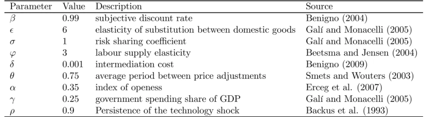
We set the subjective discount rate β = 0.99, which implies a steady state real interest rate
slightly above4%(in a quarterly model). In the empirical literature there is no consensus about the Frisch-elasticity of labour supply 1/ϕ. Following Canzoneri et al. (2005) empirical studies find values between 2.8 and 20, while Galí et al. (2001) argue that the values should be between 1 and 10. As a benchmark we will follow Beetsma and Jensen (2004) and setϕ= 3, which implies a labour supply elasticity of 1/3. The degree of price stickiness is given by θ = 0.75, so price contracts last on average for one year (Smets and Wouters (2003)). This value is consistent with empirical results.18 In line with Galí and Monacelli (2005) we set the steady state markupµ= 1.2,
1 8Dhyne et al. (2005) [θbetween 0.75-0.8] and Galí et al. (2001) [θbetween 0.67-0.81] find empirical support for this value results in the Euro area.
Parameter Value Description Source
β 0.99 subjective discount rate Benigno (2004)
ǫ 6 elasticity of substitution between domestic goods Galí and Monacelli (2005)
σ 1 risk sharing coefficient Galí and Monacelli (2005)
ϕ 3 labour supply elasticity Beetsma and Jensen (2004)
δ 0.001 intermediation cost Benigno (2009)
θ 0.75 average period between price adjustments Smets and Wouters (2003)
α 0.35 index of openess Erceg et al. (2007)
γ 0.25 government spending share of GDP Galí and Monacelli (2005)
ρ 0.9 Persistence of the technology shock Backus et al. (1993)
Table 1: Calibration of the model.
which implies that the elasticity of substitutionǫis equal to 6. In the benchmark calibration we assume a unitary coefficient of risk sharingσ implying a log utility function. Following Benigno (2009) we set δ = 0.01which implies a 10 basis point spread of the domestic interest rate over the foreign one. For the government share of outputγwe assume a value of 0.25. This value is in line with Galí and Monacelli (2005) and roughly consistent with European data. The elasticity of substitution is a critical parameter in open economy models. Obstfeld and Rogoff (2000) assume values between 3 and 6, while the Real Business Cycle literature generally uses lower values, see e.g. Chari et al. (1998), who suggest values between 1 and 2. We assume a elasticity between
home and foreign goods η = 3 (Obstfeld and Rogoff (1998)), but we also check the robustness
of the results for different parameterizations of η. Finally, cost push shocks are assumed to be i.i.d. and technology shocks follows the following AR(1) process with persistence parameter
ρa =ρa∗ = 0.8. Standard deviations of cost push shocks is 0.005 and of productivity shock it is
0.0075.
3
Discretionary Equilibria
We start with the benchmark inflation targeting regime and discuss arising discretionary equi-libria. We then continue with the extreme case of a ‘soft peg’ as this is the most simple setting to discuss problems that might arise if a country targets exchange rate. We intentionally ignore all other possible targets of the central bank for simplicity and clarity. We then check for ro-bustness of our results. Finally we investigate the intermediate case of ‘partial’ exchange rate targeting where the central bank puts some weight in its loss function to exchange rate deviations additionally to the standard inflation targeting regime.
3.1
Inflation Targeting Regime
In the inflation targeting regime the policymaker uses the social welfare functionWS
t . The
evo-lution of the economy can be rewritten in gap form as:
βdt+1 = dt−α(1−γ) ˆCt+α(1−γ) (η(2−α)−1) ˆSt+α(1−γ) ˆCt∗ ˆıt = Sˆt+1−Sˆt+πH,t+1−δdt+1+ ˆı∗t ˆ Ct = Cˆt+1− 1 σ ˆıt− EtˆπH,t+1−α ˆ St+1−Sˆt πHt = βEtπHt+1+λ(σ+φ(1−α) (1−γ)) ˆCt+λα(1 +φη(2−α) (1−γ)) ˆSt +λφα(1−γ)π∗t +ηt
where we substituted all static equations and left only dynamic relatonships.
There is only one predetermined endogenous state variable, net foreign assets dt, three
non-predetermined endogenous state variables,Cˆt, πHtandSˆt,one instrumentˆıt,and two shocks, ηt and η∗t,wherebyˆı∗t,Cˆt∗ and π∗t are all functions ofη∗t.
3.1.1 The Two Equilibria
The baseline calibration leads to two stable discretionary equilibria under the policy of home inflation targeting. The upper panel of Figure 1 demonstrates, that following an initial current account deficit the economy can follow one of the two transition paths, both of which satisfy the first-order conditions for optimality and time-consistency. They correspond to the two IE-stable discretionary equilibria described in the Appendix B. The corresponding adjustment paths are plotted using either solid or dashed lines.
When the economy starts out of the steady state with a negative net assets position the household will wish to adjust. The household will choose consumption and prices, taking into account the future paths of the interest rate as well as the state of the economy. The policymaker will use its policy instrument, the interest rate, to help to steer the economy back to the steady state; he will choose the interest rate optimally, based on the forecast of the reaction of the household to the policy and to the state of the economy.
Choosing the adjustment paths the household can foresee that the negative position in net foreign assets can be closed either quickly, if the interest rate falls sharply with a consequent depreciation of domestic currency, trade surplus and accumulation of net foreign assets, or it can be closed slowly if the interest rate rises only slightly with only a small consequent fall in consumption and therefore a slow accumulation of net foreign assets. Depending on whether adjustment is expected to be slow or fast, the private sector will set corresponding expectations and appropriate prices. It will be optimal for the policymaker to validate beliefs that prevail. Two equilibria might arise.
These different adjustment paths can be explained by the multiplicity of policy-induced private sector equilibria, see Blake and Kirsanova (2008). Essentially, for every policy there is more than one locally optimal response of the private sector, which is of course, conditional on the forecast of future policy. In order to understand how multiplicity arise we can look at the role which consumption and the terms of trade play in the determination of the law of motion for marginal
costs. After some algebra, the marginal cost can be written out as:
mct= (σ+φ(1−α) (1−γ)) ˆCt+α(1 +φη(2−α) (1−γ)) ˆSt.
It is apparent that consumption and the terms of trade are strategic complements in the control of inflation. When a positive cost-push shock hits the system the policymaker rises the interest rate and consumption is cut. Terms of trade improve. Households will use the current account to smooth consumption and decumulate net foreign assets The improved terms of trade reduce marginal cost even further. In other words, following an interest rate increase, the effect of consumption on the terms of trade reinforces the effect of the interest rate on the terms of trade, so we have a strategic complementarity as defined, for example, in ?. Multiplicity of the
policy-induced private sector equilibria becomes a likely outcome: household may choose to react in several possible ways — here they are ‘slow’ and ‘fast’ — each of them is consistent with a given policy forecast. Of course, the policymaker will react differently in response to different household actions, but the household will update their forecasts of policy in both scenarios. We end up with two discretionary equilibria and the policymaker validates beliefs in each particular equilibrium. In presence of the two equilibria, coordination failure happens: the household and the private sector can choose any of the two. A sunspot decides which one will realise as we discuss in more details in the next section.
In order to illustrate the mechanism in a stochastic setting, we plot the impulse responses to a unit cost push shock in the home economy in the middle panel of Figure 1. The shock is absorbed via a temporary fall in home output and consumption and by an initial jump in home inflation rate. The central bank fights inflation through an increase in the interest rate. After the shock, output and consumption converges to their steady states and the price level converges as well to the steady state through periods of (a very small) deflation. Households use the current account as a risk-sharing tool and sell foreign assets to dampen the decline in consumption. Therefore the country will run a current account deficit. The fall in output improves the home country terms-of-trade (ToT appreciate). As described above the baseline calibration produces two stable discretionary equilibria. The slow adjustment solution to the problem is to raise the nominal interest rate sharply, resulting in a fall in demand, low inflation and a sharp appreciation of domestic currency. As a result the value of net foreign assets will be sharply reduced first and then gradually accumulated back to the initial level while the other variables stay close to their equilibrium levels in subsequent periods.
If the economy is hit by an external cost-push shock, the foreign interest rate is raised, foreign consumption falls, the terms of trade improves and the value of foreign bonds increase. The home interest rate is raised in both regimes and therefore enforces the decline in consumption. In the slow regime it is raised by less. This results in a lower decline of consumption and therefore a stronger accumulation of net foreign assets, a small deflation and still depreciated terms of trade. When the interest rate is moved down below the baseline this results in higher inflation, small improvement of the terms of trade and still a higher foreign asset position. The accumulated net foreign assets converge slowly to the steady state in the second period and the consequent
accumulate and domestic inflation becomes negative. The positive position in net foreign assets causes consequent depreciation of the terms of trade, high inflation and overall price level stability. Note that the nominal exchange rate does not converge back to its initial value in any of the stochastic regimes. The terms of trade are stabilised, but both price level and the nominal exchange rate are unit root variables.
The responses to a positive cost-push shock for both cases look as if they were produced by the application of the classic problem of ‘dry’ and ‘wet’ policymakers (Barro and Gordon (1983)), adapted for a dynamic setting (see e.g. the discussion of the conservative central bank proposal in a dynamic setting in Clarida et al. (1999), p. 1677). In both scenarios, the interest rate rises in response to the shock, but in one scenario it rises by much more. As a result, and as in the ‘dry’ versus ‘wet’ example, we have the bigger fall in output and less inflation in the first scenario than in the second. However, rather differently from the classic problem, we have two locally optimal responses underidentical policy objectives.
Based on our observations, the two discretionary solutions can also be seen as the product of ‘seemingly patient’ respectively ‘seemingly impatient’ policymakers, with their degree of patience determined by the speed of the adjustment process of the economy back to the steady state. This distinction has nothing to do with the discount factor in the objective functions, as they remain the same. As we argue next, households/ firms make decisions based on the forecast of future policy: They either decide to bear or not the cost of adjustment. Theprivate sector, thus, chooses the equilibrium. The policymaker has no choice but to validate the forecast. We will investigate this in the following section in more detail.
3.1.2 Policy traps and equilibrium selection
Table 2 reports the welfare losses for the baseline calibration for different regimes. We claim that despite there is a clear difference in welfare ranking of the two regimes, the discretionary policymaker is unable to choose the one which yields the highest welfare. Multiplicity can only exist if there is a multiplicity of beliefs, shared by the private sector and the policymaker, about the future course of policy. The discretionary policymaker is unable to manipulate the private sector’s beliefs in order to choose the best equilibriumglobally. To understand this, it is instructive to compare what is happening in commitment and discretionary equilibria. Under commitment the policymaker is able to manipulate the private sector’s expectations alongthe whole future path, and thus, by implication, is able to choose the best path for all variables including beliefs. The discretionary policymaker is only able to manipulate private sector beliefswithina single periodt. This is because the discretionary policymaker acts as anintra-period Stackelberg leader, see Cohen and Michel (1988), sections 4 and 5. However, the policy choice in period thas to be consistent with (or conditional on) beliefs set inprevious periods if there areendogenouspredetermined state variables in the model. These past-period beliefs cannot be changed retrospectively. Once they are set their effect is long-lasting and so at time t the policymaker has to take into account the future evolution of the economy which has been affected by beliefs set prior to periodt. (Again,
unlike the case of commitment there is no ‘period 0’ when a policymaker has the power to ‘change everything’ irrespective of history.) In this sense, the private sector ‘traps’ the policymaker in a particular equilibrium.
1 2 3 4 5 0 0.5 1 ToT 1 2 3 4 5 −1 −0.5 0 NFA 1 2 3 4 5 −1 −0.5 0 Interest Rate DETERMINISTIC MODEL 1 2 3 4 5 0 0.5 1 Inflation 1 2 3 4 5 0 0.5 1 Consumption 1 2 3 4 5 −2 0 2 Nominal ER 2 4 −2 −1 0 NFA 2 4 0 1 2 Interest Rate
STOCHASTIC MODEL: DOMESTIC COST PUSH SHOCK
2 4 0 0.5 1 Inflation 2 4 −2 −1 0 ToT 2 4 −2 −1 0 Consumption 2 4 −2 −1 0 1 Nominal ER 2 4 −2 −1 0 CU 2 4 −3 −2 −1 0 Output 2 4 0 1 2 NFA 2 4 0 1 2 Interest Rate
STOCHASTIC MODEL: EXTERNAL COST PUSH SHOCK
2 4 −1 −0.5 0 Inflation 2 4 0 0.5 1 1.5 ToT 2 4 −3 −2 −1 0 Consumption 2 4 −1 0 1 Nominal ER 2 4 0 0.5 1 1.5 CU 2 4 −2 −1 0 1 Output
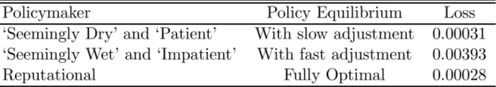
Policymaker Policy Equilibrium Loss
‘Seemingly Dry’ and ‘Patient’ With slow adjustment 0.00031
‘Seemingly Wet’ and ‘Impatient’ With fast adjustment 0.00393
Reputational Fully Optimal 0.00028
Table 2: Welfare Loss.
Their evolution is determined by consumption/ output and the terms of trade (and thus by price-setting behaviour). Consumption and prices are chosen based on the forecasted path of all variables including foreign assets. The household (who owns all firms too) is either willing or not to adjust prices and consumption in response to a shock. Its choice depends on beliefs about how quickly any adjustment will happen, and only on this. The household does not face such a choice in a world with perfect financial markets, i.e. with no predetermined endogenous variables. In this case the economy once disturbed converges back to the steady state within a single period. All monetary policy can do is to reduce theamplitude of theimmediate reactions of economic variables to shocks. The feedback coefficient of the policy rule on the observed shocks is responsible for this reduction. If there are predetermined variables in the system, then policy can also reduce the half-life of the effects of shocks already in the system. This stabilization effectively reduces the size of the non-explosive non-zero eigenvalues of the system under control. The feedback coefficients of the endogenous predetermined variables are responsible for this.
These two tasks are completely orthogonal to each other, i.e. two rules which only differ in the feedback coefficients on shocks will ensure the same half-life, and two rules which only differ by feedback coefficients on predetermined (dynamic) states will identically reduce the amplitude of concurrent shocks. The private sector can perceive the policymaker as either being ‘quick’ or ‘slow’ to stabilize the economy. These expectations decide about the first-period position in foreign assets. In turn, these expectation affect the economy more than one period into the future, as they are embedded in the dynamics of the net foreign assets. Any implied future dynamics of the economy are necessarily taken into account by future policy. The impulse responses to a cost-push shock in Figure 1 certainly resemble a policymaker that is either ‘dry/patient’ or ‘wet/impatient’. However, this is because the policymaker has to use the initial movement in interest rates to offset private sector perceptions of bringing back the economy either ‘quick’ or ‘slow’ to its steady state; the policymaker has to stick to this policy in the future.
In what follows we will term these equilibria as quick/fast and slow.
3.2
Nominal Exchange Rate Targeting
As a second extreme case we look at a ‘soft peg’. We completely ignore other targets, which may not be realistic, but the resulting regime is a useful simplification to illustrate our main point.
Under the ‘soft peg’, the reduced form system in log-linearised form can be written as: βdˆt+1 = dˆt−α(1−γ) ˆCt+α(1−γ) (η(2−α)−1) ˆ Et+ ˆpH,t−pˆ∗t +α(1−γ) ˆCt∗, ˆıt = ˆı∗t + ˆEt+1−Eˆt−δdˆt+1, ˆ Ct = Cˆt+1− 1 σ ˆıt−(1−α) ˆπHt+1−α ˆ Et+1−Eˆt , ˆ πHt = βEtπˆHt+1+λ(σ+φ(1−α) (1−γ)) ˆCt+λα(1 +φη(2−α) (1−γ)) ˆ Et+ ˆpH,t−pˆ∗t +λφα(1−γ) ˆCt∗+λφγGˆt−λ(φ+ 1) ˆAt+ηt, ˆ pH,t = ˆpH,t−1+ ˆπH,t.
Different from the version in the previous section there are two predetermined endogenous state variables: net foreign assets and the price level, dˆt and pˆH,t−1.The non-predetermined variables areEˆt,πˆH,tand Cˆt.Unlike under inflation targeting, we cannot substitute the nominal exchange rate and the price level into only one variable, the terms of trade. We have to account for the dynamics of the nominal exchange rate separately because it is the goal variable of the policymaker.
3.2.1 The ‘soft peg’
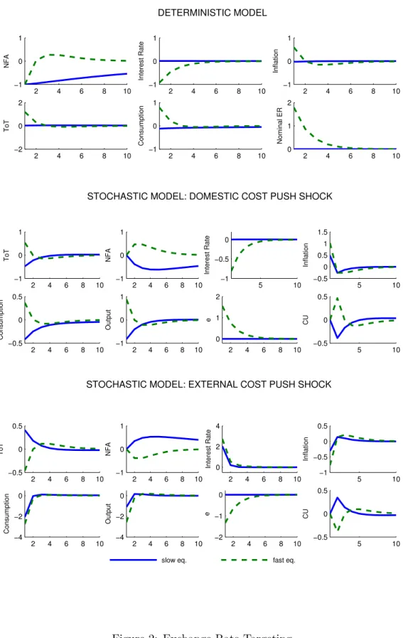
We start with the claim that under the ‘soft peg’ it is possible to keep the exchange rate on target all the time.19 Suppose we are in the derministic version of the model and the economy
starts with an excessive foreign debt. This scenario is plotted in the upper panel of Figure 2 by the solid line. In order to steer the economy back to the steady state the policymaker moves the interest rate based on the forecast of the future net foreign asset position and of the expected future depreciation. If there is a common belief that the nominal exchange rate will remain in the steady state in the future, it will be optimal for the policymaker to raise interest rate by little, to offset the forecasted δdt+1. There will be slight fall in consumption and inflation. As a result, a
small increase in savings will dominate the effect of improvement in the terms of trade on the net foreign assets. The net foreign assets will grow by little in the next period and this will require a small positive interest rate until the process converges to the steady state. The nominal exchange rate will remain in the steady state, i.e. the forecast will be validated by the policymaker.
However, the equilibrium with stable nominal exchange rate is not the only equilibrium. The second possible adjustment path is plotted in the upper panel of Figure 2 with a dashed line. Following an initial foreign debt and if there is a commonly shared belief in future appreciation of the nominal exchange rate, it is optimal for the central bank to reduce interest rate sharply, causing immediate currency depreciation and a rise in consumption and inflation. The terms of trade worsens and savings rise. This results in quick accumulation of foreign assets. A higher level of foreign assets pushes the optimal interest rate to fall even further. In other words, there is a complementarity between the interest rate and foreign assets: a reduction in the interest rate raises foreign assets that require again a lower equilibrium interest rate. With complementarities,
The ‘soft peg’ requires that the price level returns to its initial level. Therefore we should observe inflation overshooting and , indeed, this is achieved in the first equilibrium by lowering the interest rate sharply. The decline in the interest rate generates an increase in consumption and a depreciation of the terms of trade which both generate an increase in the value of the stock of net foreign assets above its steady state level. When the interest rate is raised back to its baseline level, this higher value of net foreign assets creates an additional pressure on the terms of trade. The terms of trade overshoot, improve and stay below their baseline level for a number of periods. The effect on marginal cost generates inflation overshooting and price level stability. The nominal exchange rate is stabilised at its initial level.
Despite it is commonly suggested that currency pegging is an efficient way to import low and stable inflation, it is apparent that in the case of a ‘soft peg’ the implied volatility of the nominal exchange rate and domestic inflation in the worst regime is higher than it is in the case of inflation targeting. This is not surprising: these are two ‘second-best’ scenarios, and there cannot be any a priori ranking between them. Also, the welfare minimisation in the ‘soft peg’ case assumes that both predetermined states (foreign assets and prices) can be out of the steady state so their volatility should be minimised ‘on average’, see Currie and Levine (1985). This is contrary to the inflation targeting regime where only one predetermined state exists.
The middle panel of Figure 2 plots the impulse responses to a domestic cost push shock. In the slow equilibrium inflation is accommodated: the interest rate is only marginally raised in response to the shock, and consumption falls only slightly. The terms of trade improve and the net foreign wealth loses in value. The negative net foreign assets position pushes the interest rate even further and consumption remains substantially below the baseline. This fall in consumption becomes large and long enough to reduce the marginal cost below the baseline, so inflation will fall sharply, the terms of trade will worsen and net foreign assets start to accumulate again. (Inflation falls sufficiently low to ensure the price level stability.) The same mechanism then works to steer the economy back to the steady state.
In the fast equilibrium inflation is also accommodated with a fall in the interest rate. If there is a common belief that the currency will appreciate in the future it is optimal for the policymaker to lower the interest rate now, create an immediate depreciation and worsen the terms of trade, which all leads to a rise in the real value of foreign assets. The expected appreciation drives private consumption down below the baseline, marginal costs follow and inflation is reduced below the baseline. The terms of trade improve and households start to decumulate net foreign assets. There will be less pressure to keep the interest rate low and the economy gradually converges back. A substantial inflation overshooting guarantees price level stability and the nominal exchange rate is on target.
Note that the existence of the second equilibrium does not depend on any credibility issues: discretionary policy is credible by construction, the policymaker has never promised to keep the nominal exchange rate on target. The policymaker has only promised to minimise volatility around the target. Therefore, it is acceptable to have deviations from the target as soon as all agents know the target. The possibility of ‘future appreciation’, i.e. different speeds of convergence towards the steady state, generates the second equilibrium.
The lower panel in Figure 2 demonstrates both equilibria if there is an external cost push shock. Again, it is possible to offset the shock completely. If there is a common belief that the nominal exchange rate will remain on target, the interest rate can be raised in order to offset the
Policymaker Policy Equilibrium Loss
Good With slow adjustment 0.0000
Bad With fast adjustment 0.0169
Reputational Fully Optimal 0.0000
Table 3: Welfare Loss under Exchange Rate Targeting
effect of the foreign interest rate on the economy. Consumption will fall, savings increase and net foreign assets will rise. As the terms of trade have become worse after the foreign cost-push shock, inflation will drive up in the second period. Consumption will rise and savings will fall so net foreign assets start to decumulate. A consequent improvement in the terms of trade ensures that the process of convergence is slow.
If, following an external cost push shock and a rise in the foreign interest rate, there is a common belief that the currency can depreciate in the future, then the policymaker has to raise the interest rate by more than if the currency is expected to be on target. This results in an immediate appreciation of the currency and an improvement in the terms of trade. The terms of trade effect dominates all other effects on the net foreign assets position — foreign assets lose in value. The improved terms of trade result in higher marginal costs and an higher inflation. The low real interest rate leads to an increase in consumption, so foreign assets start to accumulate and the economy eventually converges back to the steady state.
Table 3 reports the losses computed in assumption that the economy starts in the steady state and is then hit by internal and external cost-push and productivity shocks. These shocks are distributed as explained in Section 2.7. As the ‘slow’ discretionary equilibrium is able to replicate the commitment equilibrium and ensures that the nominal exchange rate is always on target, the loss in this equilibrium is identically equal to zero. In the ‘fast’ equilibrium the loss is substantially different from zero.
3.2.2 Partial Exchange Rate Targeting
Suppose a country with true flow social welfare metric
WtΠ=π2t+ωyyt2
decides to put an additional weight on nominal exchange rate targeting (provided that the anchor country pursues price stability) and chooses
Wt=π2t +ωyy2t +ωeEˆt2 (29)
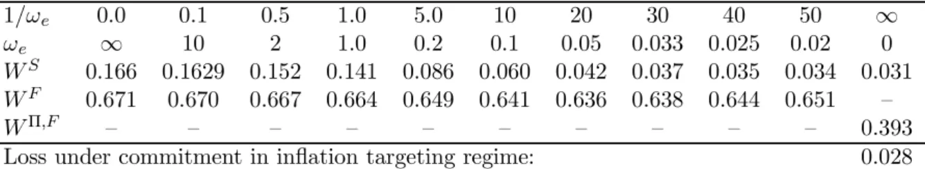
as flow objective. Table 4 reports four results. In every line we measure the implied social loss as a function ofωe.
In contrast to the commitent case under discretion adding additional targets to social ob-jectives can improve the overall policy outcome. There are many known examples of ‘optimal
2 4 6 8 10 −1 0 1 NFA 2 4 6 8 10 −1 0 1 Interest Rate DETERMINISTIC MODEL 2 4 6 8 10 −1 0 1 Inflation 2 4 6 8 10 −2 0 2 ToT 2 4 6 8 10 −1 0 1 Consumption 2 4 6 8 10 0 1 2 Nominal ER 2 4 6 8 10 −1 0 1 ToT 2 4 6 8 10 −1 0 1 NFA 5 10 −1 −0.5 0 Interest Rate
STOCHASTIC MODEL: DOMESTIC COST PUSH SHOCK
5 10 −0.5 0 0.5 1 1.5 Inflation 2 4 6 8 10 −0.5 0 0.5 Consumption 2 4 6 8 10 −1 0 1 Output 2 4 6 8 10 0 1 2 e 5 10 −0.5 0 0.5 CU 2 4 6 8 10 −0.5 0 0.5 ToT 2 4 6 8 10 −1 0 1 NFA 2 4 6 8 10 0 2 4 Interest Rate
STOCHASTIC MODEL: EXTERNAL COST PUSH SHOCK
5 10 −1 −0.5 0 0.5 Inflation 2 4 6 8 10 −4 −2 0 Consumption 2 4 6 8 10 −4 −2 0 Output 2 4 6 8 10 −2 −1 0 e 5 10 −0.5 0 0.5 CU
slow eq. fast eq.
1/ωe 0.0 0.1 0.5 1.0 5.0 10 20 30 40 50 ∞
ωe ∞ 10 2 1.0 0.2 0.1 0.05 0.033 0.025 0.02 0
WS 0.166 0.1629 0.152 0.141 0.086 0.060 0.042 0.037 0.035 0.034 0.031
WF 0.671 0.670 0.667 0.664 0.649 0.641 0.636 0.638 0.644 0.651 —
WΠ,F — — — — — — — — — — 0.393
Loss under commitment in inflation targeting regime: 0.028
Table 4: Welfare Loss under the Partial Exchange Rate Targeting, multiplied by 100. social welfare for the partial exchange rate targeting scenarios for the two equilibria, slow and fast (S andF). It is apparent that the social loss monotonically rises withωe in the slow equilibrium.
The social loss in the fast equilibrium can be slightly reduced with an appropriate choice of
ωe (ωe= 0.05). However the improvenment is only marginal.
Note that if ωe = 0 then the fast equilibrium does not exist: we are in the regime of pure
inflation targeting, with two different equilibria, but the ‘wet/impatient’ equilibrium cannot be obtained from the fast equilibrium under the partial exchange rate targeting by tendingωeto zero.
We report the lossWΠ,F in the fivth line for comparison — this is the loss in the wet/impatient
equilibrium under the pure inflation targeting. Note that in line with 3.2 the welfare losses for the fast equilibrium are higher in the partial exchange rate targeting regime than in the pure inflation targeting regime
In summary, adding the nominal exchange rate target to the policy objective can only mar-ginally improve the outcome if the economy is in the worst equilibrium. However the relative improvement is relatively small and also much smaller than in important examples in the litera-ture (‘optimal delegation’ as price-level targeting, interest rate smoothing or speed-limit policy). We therefore conclude that exchange rate targeting does not solve ‘the problem of optimal dele-gation’.
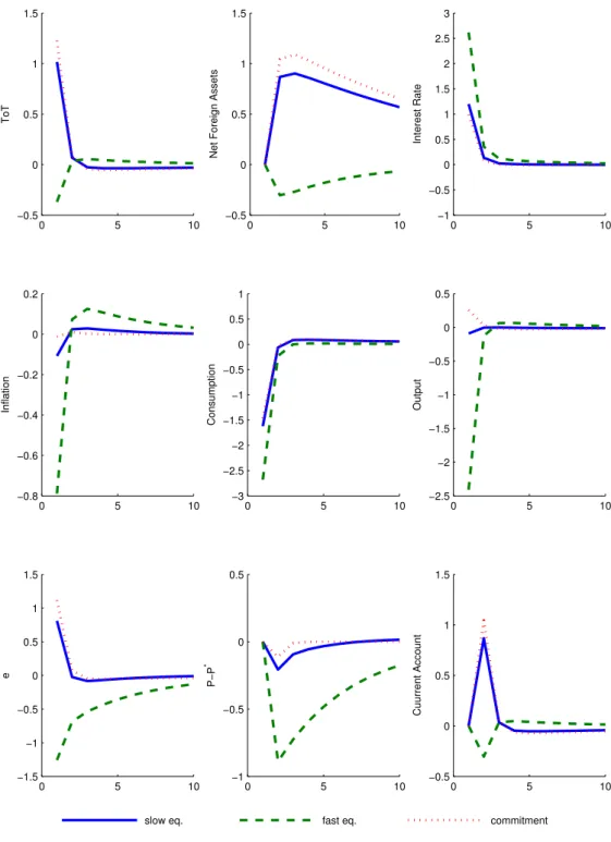
Figure 3 plots the impulse responses of an external cost push shock under the three regimes. The dotted line plots the commitment solution under pure inflation targeting (i.e. usingthe social welfare function). This the best possible outcome. The solid and the dashed lines demonstrate responses under discretion when the policymaker imposesωe= 0.05.
4
Conclusion
This paper demonstrates how a mainstream open economy model with incomplete financial mar-kets can have multiple equilibria under discretionary monetary policy. A policymaker with a given objective can choose to stabilize the economy either slowly or quickly. Depending on pri-vate sector beliefs how fast the economy will adjust back to its steady state one of these equilibria will prevail.
The model is capable of explaining recent empirical evidence on exchange rate behaviour: there can be switches in regime that are characterized by changes in nominal exchange rate volatility.
0 5 10 −0.5 0 0.5 1 1.5 ToT 0 5 10 −0.5 0 0.5 1 1.5
Net Foreign Assets
0 5 10 −1 −0.5 0 0.5 1 1.5 2 2.5 3 Interest Rate 0 5 10 −0.8 −0.6 −0.4 −0.2 0 0.2 Inflation 0 5 10 −3 −2.5 −2 −1.5 −1 −0.5 0 0.5 1 Consumption 0 5 10 −2.5 −2 −1.5 −1 −0.5 0 0.5 Output 0 5 10 −1.5 −1 −0.5 0 0.5 1 1.5 e 0 5 10 −1 −0.5 0 0.5 P−P * 0 5 10 −0.5 0 0.5 1 1.5 Cuurrent Account
slow eq. fast eq. commitment
We have also shown that the introduction of nominal exchange rate targeting into the policy objective of a discretionary policymaker does not solve the ‘optimal delegation’ problem — it only leads to higher social losses.
A
Discretionary Policy in LQ RE Models
Our linearized model equations comprise a linear rational expectations model; the criterion
functions that our central bank will minimise are all quadratic. Our problem is therefore a
special case of a general class of linear-quadratic rational expectations regulator problems. In this short section, we describe this general class of problems, and the types of equilibria that arise, formally.
We assume a non-singular linear deterministic rational expectations model of the type de-scribed by Blanchard and Kahn (1980), augmented by a vector of control instruments. Specifi-cally, the evolution of the economy is explained by the following system:20
yt+1 xt+1 = A11 A12 A21 A22 yt xt + B1 B2 [ut], (30)
whereytis ann1-vector of predetermined variables with initial conditionsy0 given,xtisn2-vector
of non-predetermined (or jump) variables, and ut is a k−vector of policy instruments of the
policymaker. For notational convenience we define the n-vector zt= (yt′, xt′)′ wheren=n1+n2.
At timetthe policymaker has the following optimization problem (Etdenotes the expectations
operator, conditional on information available at timet):
min
ut EtWt (31)
with the loss function
Wt= 1 2 ∞ s=t βs−tg′ sQgs= 1 2 ∞ s=t βs−tz′ sQzs+ 2zs′P us+u′sRus , (32)
subject to system (30). In addition, any solution to this optimization problem should satisfy the time-consistency constraint: for any s > tthe policymaker will choose
us=Etus. (33)
The elements of the vector gs are the goal variables of the policymaker, gs =C(zs′, u′s)′. Matrix
Qis assumed to be symmetric and positive semi-definite. In our formulation the quadratic loss function includes instrument costs, but no assumptions about the invertibility ofRneed be made.
We are looking for solutions that ensure that the loss is finite, i.e. Wt<∞.
The sequence of actions within a period is as follows. In the first stage of every periodt the policymaker chooses the instrument ut, knowing the state yt and taking the process by which
xt.The optimal xt, ut and given yt result in the new level ofyt+1 by the beginning of the next
periodt+ 1.
It can be proved the solution in any time t gives a value function which is quadratic in the state variables,
Wt= 1
2y
′ tSyt
and a pair of linear rules
ut = −F yt, (34)
xt = −Jyt−Kut=−(J −KF)yt=−Nyt (35)
where K=−∂xt/∂ut : in a leadership equilibrium the follower treats the leader’s policy
instru-ment parametrically. MatrixF describes the policy reaction of the policymaker, i.e. it=−F dtin
our benchmark case. Matrix N defines the reduced form reaction function of the private sector,
i.e. (st, πHt, ct)′ =−Ndt.
Definition 1 The system of first order conditions to optimization problem (30)-(33) for matrices
{N, S, F} can be written in the following form:
S = Q∗+βA∗′SA∗−P∗′+βB∗′SA∗′F, (36) F = (R∗+β′B∗SB∗)−1P∗′+βB∗′SA∗, (37) N = (A22+NA12)−1((A21−B2F) +N(A11−B1F)), (38) Q∗ = Q11−Q12J −J′Q21+J′Q22J, P∗=J′Q22K−Q12K+P1−J′P2, (39) R∗ = K′Q22K+R−K′P2−P2′K, A∗=A11−A12J, B∗=B1−A12K, (40) J = (A22+NA12)−1(A21+NA11), K= (A22+NA12)−1(B2+NB1). (41)
The proof can be found in e.g. Blake and Kirsanova (2008). There is a one-to-one mapping between equilibrium trajectories and{ys, xs, us}s∞=tand the triplet T ={N, S, F}, so it is
conve-nient to continue with definition of policy equilibrium in terms of T, not trajectories. Hence, in what follows it is convenient to use the following definition.
Definition 2 A triplet T ={N, S, F} is a discretionary equilibrium if it satisfies the system of FOCs (36)-(41).
It is apparent from system (36)-(41) that matricesN,SandF satisfy three quadratic algebraic
matrix equations (Riccati equations) (36)-(38), where the coefficients in these equations are also non-linear functions of model matrices and matrixN.This makes the whole system (36)-(41) very non-linear and it is not surprising that it may have many solution triplets TJ ={NJ, SJ, FJ}, J = 1, ..M where M is the total number of solutions. We investigate properties of these
discre-tionary solutions in Blake and Kirsanova (2008).
Oudiz and Sachs (1985) and Backus and Driffill (1986) iterative procedures search for solutions to the system of first order conditions (36)-(41) but can only find those that are asymptotically stable fixed points of corresponding recursions. Blake and Kirsanova (2008) call them R-stable. These equilibria can be deduced by rational agents if they use backward induction. In what follows we shall only consider R-stable equilibria.
B
Discretionary Equilibria
B.1
The system in the matrix form
We can substitute out all static variables in order to come to the following reduced form lineaim-prespE2.epsptimization problem, written in a matrix form. The objective function can be written as: 1 2 ∞ s=t βs−t st πHt ct ′ α2η2ω(2−α)2(1−γ)2 0 αηω(1−α) (1−γ)2 0 1 0 αηω(1−α) (2−α) (1−γ)2 0 ω(1−α)2(1−γ)2 st πHt ct .
We optimize the objective function subject to the dynamic system:
dt+1 st+1 πHt+1 ct+1 = 1 β α β(1−γ) (η(2−α)−1) δ β ακ(φη(2−α)(1−γ)+1) β + αδ(1−γ)(η(2−α)−1) β + 1 0 −ακ(φη(2−αβ)(1−γ)+1) −σβαδ ακ(1−α)(φη(2σβ−α)(1−γ)+1)−α2δ(1−γ)(σβη(2−α)−1) · ·· · · · 0 −αβ (1−γ) −β1 κ(σ+φ(1−βα)(1−γ))−αδ(1β−γ) 1 β − κ(σ+φ(1−α)(1−γ)) β −(1σβ−α) α2δσβ(1−γ) +κ(1−α)(σ+φσβ(1−α)(1−γ))+ 1 dt st πHt ct + 0 1 0 (1−α) σ [it],
Variablesct, πHt and sare non-predetermined, whiledt is a predetermined variable andit is the
instrument of the policymaker. The system matrices needed for computation are:
A11= 1 β , A12= α β (1−γ) (η(2−α)−1) 0 − α β (1−γ) , B1 = [0], A21= δ β 0 −σβαδ , B2= 1 0 (1−α) σ , A22= ακ(φη(2−α)(1−γ)+1) β + αδ(1−γ)(η(2−α)−1) β + 1 − 1 β κ(σ+φ(1−α)(1−γ)) β − αδ(1−γ) β −ακ(φη(2−αβ)(1−γ)+1) β1 −κ(σ+φ(1−βα)(1−γ)) ακ(1−α)(φη(2−α)(1−γ)+1) σβ − α2δ(1−γ)(η(2−α)−1) σβ − (1−α) σβ α2δ(1−γ) σβ + κ(1−α)(σ+φ(1−α)(1−γ)) σβ + 1 , Q11= [0], Q12=' 0 0 0 (, Q21=Q′12, and R= [0], P1= [0], Q22= α2η2ω(2−α)2(1−γ)2 0 αηω(1−α) (2−α) (1−γ)2 0 1 0 αηω(1−α) (2−α) (1−γ)2 0 ω(1−α)2(1−γ)2 , P2 = 0 0 0 .
B.2
The policymaker’s reaction function and the value function
Suppose the reaction of the private sector can be written in