Instructions for use
Author(s) Hayakawa, Hitoshi
Citation Journal of economic interaction and coordination, 13(1), 9-50https://doi.org/10.1007/s11403-017-0208-1
Issue Date 2018-04
Doc URL http://hdl.handle.net/2115/70765
Rights © 2017 Hitoshi Hayakawa.
Rights(URL) https://creativecommons.org/licenses/by/4.0/
Type article
https://doi.org/10.1007/s11403-017-0208-1 R E G U L A R A RT I C L E
Does a central clearing counterparty reduce liquidity
needs?
Hitoshi Hayakawa1
Received: 31 March 2016 / Accepted: 8 November 2017 / Published online: 16 November 2017 © The Author(s) 2017. This article is an open access publication
Abstract This study investigates whether and how central clearing influences the overall liquidity needs in a network of financial obligations. Utilizing the approach of flow network theory, we show that the effect of adding a central clearing counterparty (CCP) is decomposed into two effects: central routing, and central netting effects. Each effect can produce different liquidity needs according to different liquidity scenarios. The analysis indicates that adding a CCP in times of financial distress successfully reduces the overall liquidity needs if and only if the netting efficiency of the CCP is sufficiently high. Furthermore, once the economy is no longer in financial distress, higher netting efficiency of the CCP could conversely increase the overall liquidity needs. The results have implications for the effectiveness of CCPs in mitigating sys-temic risk in times of financial distress, and their operating costs once the distress has passed.
1 Introduction
In the recent financial crisis, the collapse of financial institutions, such as Bear Stearns and Lehman Brothers, demonstrated that the interconnected feature of bilateral expo-sure among financial institutions could lead to market disruption. In order to cope with this apparent vulnerability, the G20 leaders agreed at the 2009 Pittsburgh Sum-mit that standardized over-the-counter (OTC) derivatives should be cleared through central clearing counterparties (CCPs). Central clearing is expected to help mitigate counterparty credit risk by removing the direct risk exposure between
counterpar-B
Hitoshi Hayakawa1 Creative Research Institution/Graduate School of Economics and Business Administration, Hokkaido University, Kita9 Nishi7, Kita-ku, Sapporo, Japan
ties, thereby reducing the systemic risk of the “domino” of defaults and relevant firesales.1
However, the success and relevant cost of central clearing is never evident. For example, CCPs typically require margin themselves in order to bear the counterparty risk arising from cleared derivative transactions. In times of financial distress, margin requirements by CCPs could trigger firesales.2Here, we should note that multilateral netting by CCPs could have already reduced relevant exposure, and have contributed to reduce the required margin compared to settlements without CCPs. The effect of CCPs on overall liquidity needs is not apparent until the two aspects are investigated in a consolidated manner.
We further argue about the operating cost of CCPs once the economy is no longer in financial distress. CCPs could affect overall liquidity needs in times of non-distress, and larger liquidity needs tend to imply larger costs, since liquidity is essentially scarce resource. In times of non-distress, when financial institutions are not in a rush to obtain liquidity, contracted trades would need less liquidity, or similarly, liquidity would circulate more efficiently among relevant financial institutions even without CCPs. Consequently, CCPs and their multilateral netting could have different effects on overall liquidity needs compared with those in times of financial distress.
In order to assess the effects of CCPs and discuss further improvements of the clear-ing mechanism, it is important to understand the essential nature of CCPs regardclear-ing how they affect overall liquidity needs in times of both financial distress and non-distress. This study develops a stylized model to probe this issue. Our focus is on how the introduction of a CCP could alter the interconnected feature of the relevant network of financial obligations, and how the change of network topology could affect overall liquidity needs. From the perspective of network topology, the introduction of a CCP serves as an additional entity itself in the relevant network, while its multilateral offsetting serves to eliminate relevant obligations. We explicitly show that the effect of a CCP is decomposed into two effects: thecentral routing effect, and thecentral netting effect, such that the total effect is essentially the addition of the two effects.
The effect of a CCP is examined on the basis of two polar liquidity scenarios. One is assumed as a situation in times of financial distress, by which liquidity circulates least efficiently. The other is assumed as a benchmark situation in times of non-distress, by which liquidity circulates most efficiently. We refer to the former situation as thebad environmentand the latter as thegood environment. We show that in the bad environment, the central routing effect is always negative, but the central netting effect is always positive. A negative central routing effect means that adding a CCP certainly increases the overall liquidity needs if there is no financial obligation to be offset by the CCP. A positive central netting effect means that larger offset amounts lead to smaller liquidity needs. This implies that the total effect of a CCP is positive
1 In this respect, Brunnermeier and Pedersen (2009) argue there is a spiral nature between funding liquidity and market liquidity, whereby the initial loss could lead to firesales, which could further exacerbate the loss. 2 The possible procyclical feature associated with margin requirements of CCPs is pointed out in Domanski et al. (2015). Rennison et al. (2016) report a real world case that suggests the procylicality; on the day after Britain’s vote for Brexit, the five of the largest clearing houses demanded $27bn in additional collateral across derivatives products.
in the bad environment when the offset amount is sufficiently large. By contrast, we show that it is possible for the central netting effect in the good environment to be negative, whereby, although counterintuitive, a larger offset amount could lead to larger liquidity needs. This is because eliminating financial obligations could effectively separate a connected network into multiple disconnected networks, thereby inhibiting the same liquidity from circulating through the whole network. We observe a trade-off of multilateral trade-offsetting regarding the overall liquidity needs. It is possible for a CCP to reduce liquidity needs during times of financial distress, thereby reducing the risk of firesales and relevant systemic risk of the “domino” of defaults. However, it could conversely increase overall liquidity needs during times of non-distress. For our benchmark situations, in order for the total effect of a CCP to be always positive in the bad environment, more than two-thirds of the relevant trading needs to be offset. Since the overall liquidity needs in the good environment could become larger in proportion to the offset amount, the trade-off could become serious.
There are two policy implications of this research. First, when central clearing is used, the expected offset efficiency for the relevant security should be examined with sufficient care, since insufficient netting efficiency could have an adverse effect. Sec-ond, possible severe trade-off associated with multilateral netting suggestsconditional utilization of a CCP. Since our analysis shows that multilateral netting could be costly at the time of non-distress but helps mitigate liquidity needs at the time of financial distress, a CCP could be used as an emergency scheme. Although it is out of the scope of this study to argue about the whole cost of such an emergency scheme, our analysis indicates there is possible merit in resolving the underlying trade-off regarding overall liquidity needs.
1.1 Relevant literature and contributions
The role of CCPs has been examined largely focusing on how much relevant expo-sure is reduced through CCPs’ multilateral nettings, supposing that smaller amount of exposure to each counterparty implies smaller counterparty risk. This study departs from the literature by examining the roles of CCPs in overall liquidity needs.
Focusing on the effect on exposure, Duffie and Zhu (2011) examine central clear-ing in derivative markets and point out the possible disadvantage of central clearclear-ing arrangements compared with bilateral clearing arrangements when central clearing is provided only within each class of derivatives. The roles of CCPs in derivative markets are debated in Bliss and Kaufman (2006), Bliss and Steigerwald (2006), and Pirrong (2009). Jackson and Manning (2007) argue about the effects of CCPs in relation to “tiering,” which refers to the ratio between the number of indirect and direct members of CCPs. The authors argue there is incentive for a “tiered” structure. Galbiati and Soramäki (2012) analyze the implications of “tiering” in terms of network topology. In view of relevant network topologies, they examine the tree structure, while more general structures matter in our liquidity context.
Several recent studies have examined the role of CCPs in affecting overall liquidity needs, in the context of how CCPs set their margins. Murphy et al. (2014) investigate
the procyclical nature of various margin models, proposing quantitative measures of procyclicality. Abruzzo and Park (2016) empirically analyze the margin-setting behavior of CCPs, and find that margin-induced procyclicality is a concern during recessions, but not during times of expansion. Miglietta et al. (2015) quantify the impact on the cost of funding in repo markets of the initial margins applied by CCPs. These studies have helped clarify the possible negative effects of CCPs on overall liquidity needs, but they have not explicitly shown how the existence of CCPs could have negative effects compared with cases without CCPs.
This study provides a stylized model that enables us to compare a situation with a CCP with that without a CCP. Our focus is on the effects of CCPs on overall liquidity needs by affecting the relevant network topology. For this purpose, we utilize liquidity problems defined in the network, which are formally represented as problems offlow network. The model and liquidity problems used in this study are based on Hayakawa (2016), who investigates settlement efficiency of gross settlements in view of network topology.3The present study serves as an application of Hayakawa (2016) to examine the role of CCPs, utilizing several basic results of the study.
Section2 presents our model. Section3 illustrates our analysis in a less formal manner. Section4 provides an overview of the results. Section5 shows our formal analysis. Section6concludes. The appendix includes proofs of the relevant results.
2 Model
There are a finite number of financial institutions that have obligations among them-selves. Each obligation is formed by the trade of either of two types of securities. One type is called thetarget security, and the other thenon-target security. The target security is traded either with a CCP or bilaterally, while the non-target security is traded bilaterally. We incorporate obligations for the non-target security in order to analyze externality of the CCP in the relevant settlements. As becomes clearer soon in this section, both types of security are assumed to be of a bond or equity type in the sense that the amount of obligation formed by each trade is fixed. The simplification serves to clarify the nature of a CCP, and has implications for the debate about CCPs in derivative contracts and relevant margin issues, which are discussed in Sect.2.4, and further in the analysis section.
We divide the process of settlements into four Stages as below.
• Stage 0: Trade formation
• Stage 1: CCP scheme/bilateral scheme
• Stage 2: Offsetting under the CCP scheme4
• Stage 3: Settlements of obligations
3 The original version of the models and liquidity problems are shown in Hayakawa (2014) with additional results, which constitutes a chapter of his doctoral thesis accepted in 2011.
2.1 Stage 0: Trade formation
At Stage 0, trades among the financial institutions are exogenously given. The contracts of the trades specify that all relevant obligations are finally settled at Stage 3. We express the obligations formed at Stage 0 utilizing a flow network representation.5
The obligations are expressed with anetwork N = V,A, f.V specifies a set ofvertices, which corresponds to|V| −1 number of the financial institutions added with onehypothetical entity. The role of the hypothetical entity is stated shortly in this section. A = {(v, v,n)|v, v ∈ V,n = 1,2, . . .}specifies a set ofarcs, where each arc(v, v,k)shows thatvhas some amount of obligation tov, andkis used as an index that distinguishes among multiple arcs for(v, v). The indices are usually not mentioned in order to avoid being notationally cumbersome. Then, f : A→ R+ expresses the amount of the relevant obligations. We assume that all the obligations for the trades of the target security are formed against the hypothetical entity. Using the introduced notations,(N = V,A, f, v∗∈ V)is exogenously given at Stage 0, which we call afinancial systemwith hypothetical entityv∗.
We confine ourselves to abalancednetwork throughout this study. We say a network
V,A, fis balanced when for each vertexv∈V, the total amount of obligations owed byvand those owed tovare equal, that is,v∈V f((v, v))=
v∈V f((v, v))for everyv ∈V. This is explicitly stated as Assumption1. The assumption of balanced networks has dual roles. On the one hand, it implies market clearing regarding the trades of the target security, since the total amount of obligations owed to and by the hypothetical entity are supposed to be equal. On the other hand, a balanced network at Stage 0 derives a balanced network at later stages. There, we examine relevant liquidity needs based on each network, and the assumption of the balanced network serves to simplify our analysis.6
Assumption 1 Given a financial system(N = V,A,f, v∗ ∈ V), network N is balanced.
We further assume that each of the obligations owed to and by the hypothetical entity is the same amount, that is, the price of the target security is supposed to be fixed, and each trade is made in the same unit. The assumption is formally stated as follows.
Assumption 2 Given a financial system(N = V,A, f, v∗ ∈ V), networkN has thecommon obligation value m >0 regarding the hypothetical entityv∗such that,
i) (obligations owed byv∗) f((v∗, v))=m, for everyv∈V such that(v∗, v)∈ A, and
5 For basic terminologies of flow networks, we obey the textbook usages. See, for example, Ahuja et al. (1993).
6 Our analysis on balanced networks could be extended to networks that are not balanced. For a non-balanced network, we could derive a non-balanced network by “local changes,” such as adding arcs and/or adjusting relevant weights. Conversely, we derive the original non-balanced network through the relevant “reverse” local changes on the balanced network. The amount of liquidity needs for the original non-balanced network could be derived by examining the effects of those “reverse” local changes on the balanced network.
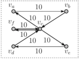
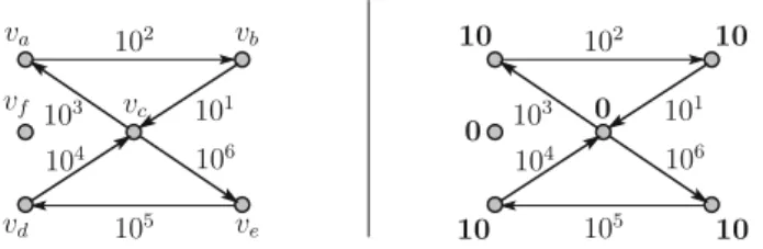
10 10 10 10 10 10 vc 10 10 va vb vd ve vf
Fig. 1 Examplefinancial systemconsistent with all the assumptions. Financial system(V,A,f, vc):
V = va, vb, vc, vd, ve, vf, A = {(va, vb), (vb, vc), (vc, va), (vc, ve), (ve, vd), (vd, vc), (vc, vf), (vf, vc)}, f(a)=10 for everya∈A 10 10 10 10 vc 10 10 va vb vd ve vf 10 10 10 10 10 10 vc 20 20 va vb vd ve vf 5 10 10 10 10 10 vc 10 10 va vb vd ve vf
Fig. 2 Examplefinancial systemsthat do not satisfy one of the assumptions. In all three financial systems, vcis assumed as the hypothetical entity. Each financial system violates one of the assumptions. The left
financial system violates Assumption1, sincevareceives 10 in total, which is larger than the total amount
of its payment 5. The middle financial system violates Assumption2, since f((vf, vc))= f((vb, vc)).
The right financial system violates Assumption3, since it indicates no trade of the target security other than those byvf
ii) (obligations owed tov∗) f((v, v∗))=m, for everyv∈Vsuch that(v, v∗)∈ A. Combined with Assumptions1and2, the next assumption ensures there are some feasiblebilateral trades for the target security, that is, if one financial institution is to buy (sell) a certain amount of the target security, at least the same amount of the target security are sold (bought) by the other financial institutions.
Assumption 3 Given a financial system(N = V,A, f, v∗∈V),
i) for everyv ∈ V\v∗, the number of “buys” of the target security byv is equal to or less than the number of “sells” of the target security by the other financial institutions. Formally,|{(v, v∗,k) ∈ A|k = 1,2, ..,}| ≤ |{(v∗, v,k) ∈ A|k = 1,2, .., v∈V, v=v}|.
ii) for everyv ∈ V\v∗, the number of “sells” of the target security by v is equal to or less than the number of “buys” of the target security by the other financial institutions. Formally,|{(v∗, v,k) ∈ A|k = 1,2, ..,}| ≤ |{(v, v∗,k) ∈ A|k = 1,2, . . . , v∈V, v=v}|.
An example financial system that satisfies all Assumptions1,2, and3is shown in Fig.1, wherevccorresponds to the hypothetical entity, and there are six obligations for the target security. For presentational purposes, obligations for the target security are shown with thicker lines, while those for the non-target security are shown with thinner lines, and this applies throughout this article. For clarification of the assumptions, Fig.2
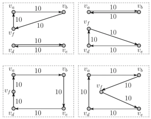
Fig. 3 Bilateral networks for the financial system shown in Fig.1 va vb vd ve vf va vb vd ve vf va vb vd ve vf va vb vd ve vf 10 10 10 10 10 10 10 10 10 10 10 10 10 10 10 10 10 10 10 10
of the assumptions. The left financial system does not satisfy Assumption1, the middle financial system does not satisfy Assumption2, and the right financial system does not satisfy Assumption3.
2.2 Stage 1: CCP scheme/bilateral scheme
At Stage 1, the hypothetical entity is materialized under either of the two schemes: the CCP scheme and the bilateral scheme. For the CCP scheme, the hypothetical entity is itself reinterpreted as a CCP for the target security. Thus, the network given at Stage 0 is unchanged. When the given network as Stage 0 is that shown in Fig.1with hypothetical entityvc,vcis reinterpreted simply as the CCP under the CCP scheme at Stage 1. Note that the CCP does not offset obligations at Stage 1, but it will do so at Stage 2. In order to simplify relevant statements, we refer to a network derived under the CCP scheme at Stage 1 as aCCP network.
For the bilateral scheme, the hypothetical entity is made to vanish, and we examine all the possible bilateral trades for the target security. We refer to networks that are derived under the bilateral scheme asbilateral networks. Specifically, when the finan-cial system shown in Fig.1is given at Stage 0 with hypothetical entityvc, we derive four bilateral networks, as shown in Fig.3. Observe that in each bilateral network, each obligation(v, vc),v ∈ {vb, vd, vf}that is previously owed to the hypothetical entity is paired with an obligation(vc, v),v ∈ {va, ve, vf}that is previously owed by the hypothetical entity, and the pair of arcs is replaced with a new arc (v, v). For the network shown on the upper-left in Fig.3, the relevant arcs are paired such that{(vb, vc), (vc, vf)},{(vf, vc), (vc, va)},{(vd, vc), (vc, ve)}, and each of the pairs is replaced by each of(vb, vf),(vf, va), and(vd, ve).
In general, for a given financial system(N = V,A, f, v∗ ∈ V), let At o ⊂ A denote a set of obligations owed to the hypothetical entity, and Aby ⊂Adenote a set of obligations owed by the hypothetical entity. Note that|At o| = |Aby|.7Consider 7 For a networkN shown in Fig.1with hypothetical entityv
c,Ato= {(vb, vc), (vd, vc), (vf, vc)}, and
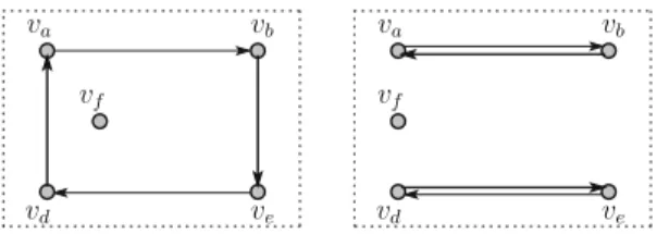
va vb vd ve vf va vb vd ve vf
Fig. 4 Networks that are not assumed as bilateral networks for the financial system shown in Fig.1. For the network shown Fig.1, each of the networks shown in the figures is derived when the pair of arcs
{(vc, vf), (vf, vc)}is replaced with the vertexvf. We do not assume these networks as relevant bilateral
networks since it effectively assumes offsetting of obligations under the bilateral scheme.
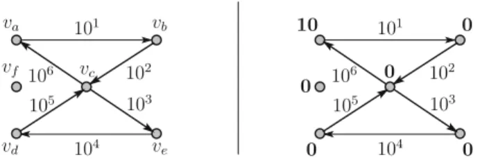
Fig. 5 The net-out CCP network for the financial system shown in Fig.1. The pair of arcs
{(vf, vc), (vc, vf)}has been
removed from the network shown in Fig.1 10 10 10 10 10 10 vc va vb vd ve vf
all the possible one-to-one matchings between At oand Aby. For each matching, let each pair of arcs{(v, v∗), (v∗, v)}, v, v ∈ V be replaced with a new arc(v, v). Here, we exclude any matching that includes a pair of arcs regarding the same vertex such that{(v, v∗), (v∗, v)},v∈V.8The reason for the exclusion of such matching is that the pair of obligations{(v, v∗), (v∗, v)}needs be replaced with vertexv, which effectively assumes offsetting between the paired obligations. We assume any bilateral or multilateral offsetting is not executed under the bilateral scheme.
In examining bilateral networks, our later analysis examines all the possible match-ings instead of focusing on any specific probable matching. In this sense, we do not make any assumption about counterparty risks conceived among financial institutions, or other factors that affect probable realization of matching.
2.3 Stage 2: Offsetting under the CCP scheme
Stage 2 is relevant only to networks derived under the CCP scheme. The CCP now offsets obligations, and we derive an associated network. For example, when we see the network in Fig.1as a CCP network with CCPvc, offsetting by the CCP derives a network shown in Fig.5, where the pair of obligations{(vf, vc), (vc, vf)}has been offset. In general, for a CCP networkN = V,A,fwith CCPv∗∈V, remove all the arcs that constitute a pair{(v, v∗), (v∗, v)}, forv∈V. We call the derived network the net-out CCP networkregardingv∗. Our aim is to compare the set ofbilateral networks and thenet-out CCP network, given the same financial system. When the given
finan-8 For networkN shown in Fig.1with hypothetical entityv
c, we exclude one-to-one matchings in which
the pair of arcs{(vf, vc), (vc, vf)}is included. Those excluded matchings would yield networks shown in
101 104 102 103 106 105 vc va vb vd ve vf 101 104 102 103 106 105 0 10 0 0 0 0
Fig. 6 Example sequence and relevant liquidity needs (1).s(va, vb)=1,s(vb, vc)=2,s(vc, ve)=3,
s(ve, vd)=4,s(vd, vc)=5,s(vc, va)=1,pva(s)=10, andpvb(s)= pvc(s)=pvd(s)= pve(s)= pvf(s)=0
cial system is a network shown in Fig.1with hypothetical entityvc, we compare the set of bilateral networks shown in Fig.3with the net-out CCP network shown in Fig.5.
2.4 Stage 3: Settlement of obligations
At Stage 3, the remaining obligations are settled on a gross basis.9Specifically, we define agross settlement for a networkN = V,A,f with one-to-one mapping (sequence)s : A→ {1,2, ..,|A||}and a set of values{pv(s)≥ 0}v∈V, in which the former shows the relative order of the settlements, while the latter shows the liquidity needs for eachv ∈ V under the order. For a network shown in Fig.5, an example sequences : A → {1,2, . . . ,6}is shown on the left side of Fig.6, in whichs(a) is written on the upper-right of the value f(a)for eacha ∈ A. The right side of the figure shows the same network to which is added the corresponding pv(s)for each
v∈V, where each value is shown in boldface. Under the specified order, the financial institution expressed asvaneeds to input 10 funds, since it has not received any liquidity before. For each of the rest of the institutions, including the CCP, the liquidity needs are shown as zero, since each has received sufficient amount of liquidity when each settles its obligation. Thus, we set{pv(s)}v∈V so that pv(s)is neither redundant nor short of the settlements for eachv∈Vunder given sequences. Formally, we explicitly set{pv(s)}v∈V in the following procedure.
• Procedure to set{pv(s)}v∈V
·LetV,A, fands: A→ {1,2, ..,|A|}be given.
·Letk=0,1,2, . . . ,show thecurrent orderfor the relevant settlements.
·Letphv(k)indicate thecurrent liquidity holding.
·Letpdv(k)indicate thecurrent liquidity needs.
• Initialization
·Setphv(0)=0 andpdv(0)=0, for everyv∈V.
·Setk=1.
9 The World Bank (2013) reports that more than 80% of the surveyed payment systems had adopted real-time gross settlement (RTGS) systems. Several interbank payment systems incorporate offsetting mechanisms into their RTGS systems, which are referred to as the liquidity saving mechanism. From this perspective, this study assumes that settlements at Stage 3 are under an RTGS system without any liquidity saving mechanism.
• Main Procedure
·Takea=(v, v)∈ Asuch thats(a)=k.
i) For thepayerv, setpdv(k)andphv(k)as follows.
· pd
v(k)=max(f(a)−phv(k−1),0),
· phv(k)=max(pvh(k−1)− f(a),0).
ii) For thereceiverv, set pvd(k)andphv(k)as follows. · pdv(k)=0,
· phv(k)= pvh(k−1)+ f(a).
iii) For the otherv∈V\{v, v}, setpdv(k)=0 and pvh(k)= pvh(k−1). ·Update the current order ask:=k+1.
·Ifk >|A|, proceed to thefinalization; otherwise, repeat themain procedurewith the updatedk.
• Finalization
·For eachv∈V, setpv(s)=k|A=|1pvd(k).
For given networkV,A, fand sequences : A → {1,2, . . . ,|A|}, we examine total liquidity needsv∈V pv(s)for our analysis. Note that we refer to liquidity needs as the amount of liquidity necessary for the relevant settlements, but not the amount of liquidity that is prepared by financial institutions from an ex-ante perspective.The purpose is to clarify liquidity needs in relation to the overall financial state, independent of expectations held by the relevant financial institutions that could depend on each individual context. The overall financial state is expressed with each of our liquidity scenarios.
2.4.1 Liquidity scenarios
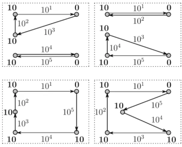
We focus on two polar types of scenario for our analysis; one is a scenario in thegood environment, and the other in thebadenvironment. The good environment refers to the financial state in which settlements are executed under the best coordination, and the overall liquidity needs is the minimum possible. By contrast, the bad environment refers to the state in which settlements are executed under the worst coordination, and liquidity needs are the maximum possible. The bad environment is meant to express liquidity needs during times of financial distress, while the good environment is used as a benchmark state in times of non-distress. Given a net-out CCP network in Fig.5, Fig.6shows a settlement in the good environment, and Fig.7shows a settlement in the bad environment for the same network.
Formally, the total liquidity needs in each environment is derived by each of the following minimization and maximization problems.
(Liquidity problem for the good environment)10
Given networkV,A, f, take one-to-one mappings : A → {1,2, . . . ,|A|}and associated{pv(s)}v∈V such that
mins
v∈V pv(s).
10 The presented minimization and maximization problems are formally introduced in Hayakawa (2016), Hayakawa (2014), and originally in his doctoral thesis. In arguing the computational aspect, the problems are specifically referred to as the (minimum/maximum) settlement fund circulation problem.
102 105 101 106 103 104 vc va vb vd ve vf 102 105 101 106 103 104 0 10 10 10 10 0
Fig. 7 Example sequence and relevant liquidity needs (2)s(va, vb)=1,s(vb, vc)=2,s(vc, ve)=3,
s(ve, vd)=4,s(vd, vc)=5,s(vc, va)=1,pva(s)=10, andpvb(s)= pvc(s)=pvd(s)= pve(s)= pvf(s)=0
Fig. 8 Settlements in the good
environment 10 0 10 0 0 10 0 0 0 10 10 0 0 0 0 10 0 0 0 0 101 103 102 104 105 101 102 105 104 103 104 101 101 105 105 10 2 103 103 104 102
(Liquidity problem for the bad environment)
Given networkV,A, f, take one-to-one mappings : A → {1,2, . . . ,|A|}and associated{pv(s)}v∈V such that
maxs
v∈V pv(s).
In other words, the liquidity problem for the good (bad) environment derives the minimum (maximum) total liquidity needs with respect to every possible order of settlements. For clarity of the problems, take the networks shown in Fig.3as inputs for each of the minimization and maximization problems. Then, Fig.8shows relevant settlements in the good environment, and Fig.9shows those in the bad environment. The bad environment could be interpreted as a panic situation that is typical in times of financial distress, whereby financial institutions try to receive their payments as early as possible, or require margin for their relevant exposure. Notice that in our model, we do not allow multiple settlements to be made simultaneously, since we assume that each different order needs to be set for each arc. That means not all the obligations are settled with additional liquidity input, as confirmed in Fig.7, where pvc =0 instead of 20. In other words, a certain positive amount of liquidity is economized even under the bad environment. This is because when the first payment is made, there is at least one institution that receives liquidity before it makes any payment. This captures the essential nature of the circulation of liquidity such that liquidity can be used once it is obtained. The good environment is treated as an ideally efficient situation in terms of
Fig. 9 Settlements in the bad environment 10 0 10 0 10 10 0 10 0 10 10 0 10 10 10 10 0 10 10 10 101 102 103 104 105 101 102 102 103 104 103 101 101 104 102 10 5 104 103 105 105
liquidity input, in which the liquidity inputs, and associated costs, are economized as much as possible.
3 Illustrative examples
We argue that the effect of a CCP needs be examined carefully in each liquidity scenario. We show that in the bad environment, a CCP increases overall liquidity needs if the netting efficiency is not sufficiently high. Still, higher netting efficiency contributes to decrease liquidity needs in the bad environment, and sufficiently high netting efficiency ensures that the CCP decreases the total liquidity needs compared to the corresponding bilateral settlements. However, when we consider the good environ-ment, higher netting efficiency does not necessarily serve to decrease overall liquidity needs. Actually, it is possible that higher netting efficiency leads to larger overall liq-uidity needs. Thus, there is a possible trade-off regarding the netting service provided by the CCP.
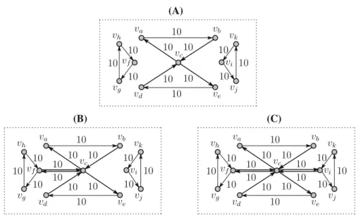
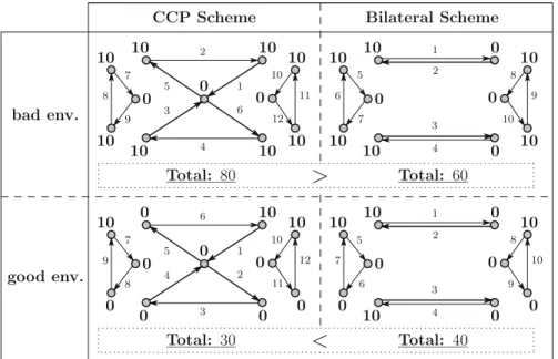
In order to illustrate the trade-off and our relevant analysis in a less formal manner, here, we examine three examplefinancial systems(A), (B), and (C), shown in Fig.10. Hypothetical entity isvcin each financial system. As easily confirmed, the amount of obligations offset by the CCP is the largest for (C), and zero for (A).
Figure 11 shows settlements for networks generated by financial system (A). Although we have more than one bilateral network, for illustrative purposes, we focus on one bilateral network shown in the figure. In the analysis section, we show results considering all possible bilateral networks for each given financial system. Figure11
shows an example order of settlements and the relevant liquidity needs for each of the two networks (a net-out CCP network and a bilateral network) in each environment. Observe that in the bad environment, the total liquidity needs are larger for the CCP scheme, while it is the same in the good environment. In the same manner, Fig.12
shows relevant settlements for financial system (B), and Fig.13shows those for finan-cial system (C). Notice that the offsetting amount increases when we move from (A) to (B) and from (B) to (C). Thus, we observe that as the offsetting amount increases,
10 10 10 10 10 10 10 10 10 10 10 vc va vb vd ve 10 10 10 10 10 vf vh vg vi vj vk (C) 10 10 10 10 10 10 10 10 10 vc va vb vd ve 10 10 10vf vh vg vi vj vk (A) 10 10 10 10 10 10 10 10 10 vc va vb vd ve 10 10 10 10 10 vf vh vg vi vj vk (B)
Fig. 10 Example financial systems. In each financial system (A), (B), and (C),vcis assumed as the
hypothetical entity
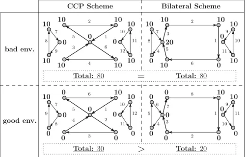
CCP Scheme Bilateral Scheme
bad env. good env. 11 12 10 0 10 10 10 10 7 9 8 0 10 10 0 10 10 1 9 10 8 5 7 3 6 2 1 5 6 3 4 2 4 10 10 10 10 0 10 0 0 10 10 11 10 0 0 10 0 0 7 8 9 0 10 0 0 0 10 6 1 5 2 4 3 12 10 9 8 5 6 7 4 2 0 10 0 0 0 0 10 10
>
Total: 80 Total: 70 Total: 30=
Total: 30 3 0 1 0Fig. 11 Financial system (A): relevant settlements. For each network, relevant order is presented for each arc and the corresponding liquidity needs are presented for each vertex. We omit the relevant amount of obligations, which is 10 for all the arcs, in this figure
the total liquidity needs under the CCP scheme become relatively smaller in the bad environment, but relatively larger in the good environment. This shows the possible trade-off of the multilateral offsetting by the CCP.
CCP Scheme Bilateral Scheme bad env. good env. 11 12 10 0 10 10 10 10 7 9 8 0 10 10 0 10 10 1 10 11 9 7 4 3 5 8 2 1 5 6 3 4 2 6 10 10 10 0 0 10 0 20 10 10 11 10 0 0 10 0 0 7 8 9 0 10 0 0 0 10 6 1 5 2 4 3 12 11 10 9 6 4 7 3 5 8 2 0 0 0 0 0 0 0 10 10
=
Total: 80 Total: 80 Total: 30>
Total: 20 1 0Fig. 12 Financial system (B): relevant settlements
CCP Scheme Bilateral Scheme
bad env. good env. 11 12 10 0 10 10 10 10 7 9 8 0 10 10 0 10 10 3 2 12 1 11 9 6 5 7 10 2 1 5 6 3 4 4 8 10 10 10 0 0 0 20 20 10 10 11 10 0 0 10 0 0 7 8 9 0 10 0 0 0 10 6 1 5 2 4 3 12 9 1 11 10 12 6 4 7 3 5 8 2 0 0 0 0 0 0 10 0 0 0
<
Total: 80 Total: 90 Total: 30>
Total: 10Fig. 13 Financial system (C): relevant settlements
The trade-off of the multilateral offsetting by the CCP is better understood by decomposing the total effect of the CCP into two types. One type is referred to as the
central routing effect, and the other as the central netting effect. The base result shown in the analysis section is summarized as follows.
CCP Scheme Bilateral Scheme bad env. good env. 11 12 10 0 10 10 10 10 7 9 8 0 10 10 0 10 10 2 9 10 8 5 7 3 6 2 1 5 6 3 4 1 4 10 10 10 10 0 10 0 10 11 10 0 0 10 0 0 7 8 9 0 10 0 0 0 10 6 1 5 2 4 3 12 10 9 8 5 6 7 1 4 10 10 10 0 0 0 0 10
>
Total: 80 Total: 60 Total: 30<
Total: 40 2 3 0 0 0 0Fig. 14 Financial system (A): relevant settlements (2)
(Total effect)=(Central netting effect)+(Central routing effect). The base result essentially states that the total effect is quantitatively decomposed into the two effects, such that the two effects are additive with each other.
3.1 Central routing effect
For financial system (A), there is no offsetting under the CCP scheme, which lets the net-out CCP network be equal to the CCP network. Thus, the total effect of the CCP for financial system (A) equals the central routing effect. Furthermore, the central routing effect of the CCP for each financial system (B) and (C) is equal to that for financial system (A), from the observation that each net-out CCP network for financial system (B) and (C) is essentially the same as the CCP network for financial system (A). This is formally shown in the analysis section.
For financial system (A) and relevant networks, as shown in Fig.11, the liquid-ity needs in the bad environment are larger for the net-out CCP network than the shown bilateral network. This also holds when we compare the net-out CCP network to another bilateral network, as shown in Fig.14. In general, we show that the central routing effect in the bad environment is strictly negative. By comparison, as indicated by the two figures, the liquidity needs for the net-out CCP network in the good environ-ment is either equal to or smaller than that for each of the relevant bilateral networks. In general, we show that the central routing effect in the good environment is weakly positive in that sense.
The intuition for the results presented above is as follows. In the good environment, the CCP tends to provide additional routes for liquidity to circulate more efficiently.
This is well illustrated in Fig.14. For the bilateral network shown on the right of the figure, there are four mutually isolated cycles of obligations. When we turn to the net-out CCP network shown on the left, we observe that the CCP serves to connect two of the previous isolated cycles to let them form one cycle. The same liquidity can now circulate throughout the united cycle. By contrast, in the bad environment, the CCP provides an additional stop for liquidity, which always increases the total liquidity needs. This is easier to observe in Fig.11. Each of the bilateral and net-out CCP networks consists of three mutually isolated cycles. The difference is that for the net-out CCP network, there is one additional vertex for one of the cycles (the cycle at the center). This actually increases the liquidity needs for the relevant cycle from 30 to 40.
The central routing effect clarifies a negative aspect of adding a CCP during times of financial distress. For the case of derivative contracts, the CCP tends to demand liquidity in the form of margin. Suppose that the relevant derivatives are traded without any CCP; then, it is possible that the direct counterparty instead of the CCP demands margin, intending to ensure counterparty risk. Suppose that for some derivative trade, the margin demanded by the CCP is the same level as that demanded by the direct counterparty; then, there is no change in the amount of the required margin for the trade itself. However, during times of financial distress when margin requirement is prevalent regardless of the types of derivatives, adding a CCP indicates that the number of institutions that require margin effectively increases in total. This is interpreted as a negative externality of adding a CCP, which is well demonstrated by the central routing effect.
3.2 Central netting effect
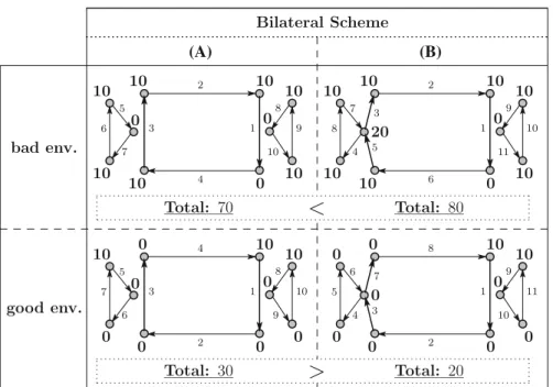
In order to observe the central netting effect for a given financial system, we take a corresponding financial network as the standard for comparison. Specifically, for each financial system (B) and (C) shown in Fig.10, the standard financial system is financial system (A). In general, for a given financial system, we take the standard financial system by offsetting all the obligations regarding the hypothetical entity. For financial systems (B) and (C), the hypothetical entity isvc, and offsetting the relevant obligations yields financial system (A). Our view is that the central routing effect for a given financial system is the same as that for its standard financial system, and the central netting effect is captured by comparing the bilateral networks for the two financial systems. For example, a bilateral network for financial system (B) shown on the right of Fig.15is compared with a bilateral network for financial system (A) shown on the left of the same figure. The way to correspond the relevant bilateral networks is shown in the analysis section. We observe there are two mutually isolated cycles in the bilateral network for financial system (B), while there are three for (A).11We consider that the original larger cycle in (B) is separated into two cycles (one with three vertices and one with four vertices) in (A). In the bad environment, the separation tends to decrease the number of stops for liquidity, and accordingly 11 Note that we refer to a cycle even when it consists of multiple cycles that are mutually connected.
(A) (B) bad env. good env. 1 10 11 9 7 4 3 5 8 2 6 10 10 0 10 0 20 10 10 11 10 9 6 4 7 3 5 8 2 0 0 0 0 0 10 10
<
Total: 70 Total: 80 Total: 30>
Total: 20 1 0 1 10 8 5 7 3 6 2 4 10 10 0 10 0 0 10 10 9 10 10 0 10 10 0 1 9 8 5 6 3 7 4 2 0 0 0 0 0 0 10 10 10 0 10 Bilateral SchemeFig. 15 Financial systems (A) and (B): networks under the bilateral scheme
decreases the liquidity needs. In general, we show that the central netting effect is weakly positive in the bad environment. By contrast, in the good environment, the separation now could increase liquidity needs. This is because the same liquidity can circulate only within each of the separated cycles. Figure16 compares a bilateral network for financial system (C) shown on the right and that for financial system (A) shown on the left, for which we confirm the central netting effect in the same manner.
Although we observe a negative aspect of the central netting effect in Figs. 15
and16, it could conversely have a positive effect. We illustrate this point using financial systems (D) and (E), shown in Fig.17. Note that (D) is the standard financial system for (E). Thus, the central routing effect for (E) is captured through (D). Figure18
shows example bilateral networks for our examination of the central netting effect. We observe that the central netting effect is positive in the good environment. We observe three mutually separated cycles for (E) and two for (D). The liquidity needs are reduced by reducing one cycle.
Suppose each of isolated verticesvf andvg in (E) forms a cycle with additional vertices and arcs through the trades of the non-target security, as is the case for financial system (C). Then, whether the central netting effect in the good environment is positive or negative depends on the amount of obligations for the non-target security. Actually, we show that it is positive when the amount of obligations for the non-target security is sufficiently small (financial system (E) is understood as an extreme case such that there is no relevant trade of the non-target security.).
(A) (C) bad env. good env. 12 1 11 9 6 5 7 10 4 8 10 10 0 0 20 20 10 10 11 10 12 6 4 7 3 5 8 2 0 0 0 0 0 0 0
<
Total: 70 Total: 90 Total: 30>
Total: 10 1 10 8 5 7 3 6 2 4 10 10 0 10 0 0 10 10 9 10 10 0 0 10 0 1 9 8 5 6 3 7 4 2 0 0 0 0 0 0 10 10 10 0 10 Bilateral Scheme 10 3 2 9 1Fig. 16 Financial systems (A) and (C): networks under the bilateral scheme
10 10 10 10 10 10 vc va vb vd ve vf (D) 10 10 10 10 10 10 vc va vb vd ve 10 10 vf (E) vg vg 10 10
Fig. 17 Financial systems (D) and (E)
On the contrary, we show that the central netting effect is negative in the good environment if the amount of each obligation for the target security is relatively small compared to that for the non-target security. This has a political implication in that the operating cost of CCPs in terms of the overall liquidity needs should not be evaluated solely from the activities of the CCPs themselves, but their external-ities on the efficiency of liquidity circulation should be considered with sufficient care.
4 Overview of the results
We briefly overview the analysis and relevant results presented in the next section. In the analysis, first, the decomposition of the total effect of adding a CCP is formally
(D) (E) bad env. good env. 2 3 5 1 6 10 10
<
Total: 20 Total: 30 Total: 20<
Total: 30 1 4 10 Bilateral Scheme 0 4 0 0 10 2 0 0 10 3 1 4 10 2 0 0 10 3 2 3 5 1 6 10 10 0 4 0 0 10Fig. 18 Financial systems (D) and (E): networks under the bilateral scheme
presented. Although we illustrate the decomposition in Sect.3using example bilateral networks for given financial system, Theorem 1 ensures that the decomposition is well defined in the sense that the decomposition is applied to all the possible bilateral networks consistently. The decomposition serves as the analytical basis for showing our relevant results.
Theorem2shows the general results for the central routing effect both in the good and bad environment, and Theorem4shows the general results for the central netting effect in the bad environment. When we focus on the results in the bad environment, the combination of Theorems2and4implies that in order for a CCP to have a positive total effect during times of financial distress, it needs to provide sufficiently high netting efficiency.
For the quantitative aspect regarding how much netting efficiency is needed for a CCP to have a positive effect in the bad environment, we introduce a specific class of financial systems to capture the interconnected feature of real world networks of financial obligations. For the specific class, Theorem3shows the quantitative aspect of the central routing effect, while Theorem5shows the quantitative aspect of the central netting effect. The results for the combined total effect are summarized in Theorem6. The theorem shows that the required netting efficiency is 66.6% for the specific class of financial systems, in order to ensure the total effect of a CCP to be positive in the bad environment . The theorem further explicitly shows the trade-off of multilateral netting by a CCP in that higher netting efficiency leads to a larger negative effect in the good environment when each obligation settled by the CCP is relatively small.
(N, v∗) (Nnet, v∗) Nnet NBnet . . . .. CCP scheme NB matching Bilateral scheme netting effect routing effect Total effect 1 4 2 3 5 central central
Fig. 19 A schematic illustration of the decomposition of the effect of a CCP. There are two types of arrows shown in the figure: thinner arrows and thicker arrows. Each thinner arrow starts from either of the financial systems, which shows the possible network under each scheme. The three thicker arrows are to illustrate the decomposition
5 Analysis
5.1 Decomposition of the effect of a CCP
We formally show the decomposition of the effect of a CCP. In order to clarify the state-ment and relevant notations, Fig.19provides a corresponding schematic illustration. Given financial system(N, v∗)(1 ), denote the network derived under the CCP scheme asNnet (2), which is referred to as thenet-out CCP networkfor(N, v∗). In an informal description,Nnetis derived from(N, v∗)by offsetting all obligations regardingv∗. Then, for the original financial system(N, v∗), take the corresponding financial system(Nnet, v∗)(3), which is referred to as anet-out financial system. Note that the net-out CCP network for the obtained net-out financial system(Nnet, v∗) is the sameNnet(2).12
Then, for each bilateral networkNB(4) for the original financial system(N, v∗) (1), we take its corresponding bilateral networkNBnet(5) for the obtained financial system(Nnet, v∗)(3). The procedure for taking correspondingNBnetis specified by (P1) provided below.
For our formal expression regarding the total liquidity needs in each environment, let xmi n(V,A,f)(xmax(V,A, f)) denote the total liquidity needs in the good (bad) environment for given network V,A, f. Specifically, xmi n(V,A, f) = mins
v∈V pv(s), and xmax(V,A, f) = mins
v∈V pv(s), using the notations defined in Sect.2.4.
The total effect of a CCP in the good environment is examined through a set of values
{xmi n(NB)−xmi n(Nnet)}with respect to every possibleNB, and the effect in the bad environment is examined in exactly the same manner. For now, suppose we have 12 The dotted line in Fig.19shows thatNnetis the same for2 and3.
somehow derived a correspondingNBnet for eachNB. We show our decomposition below, which states that for eachNB, the total effect a CCP is decomposed into two effects based on each correspondingNBnet.
Decomposition of the effect of a CCP
(Total effect)=(Central Netting effect)+(Central Routing effect).
·xmi n(NB)− xmi n(Nnet) = (xmi n(NB)− xmi n(NBnet)) +(xmi n(NBnet)− xmi n(Nnet)).
·xmax(NB)−xmax(Nnet) = (xmax(NB)−xmax(NBnet))+(xmax(NBnet)− xmax(Nnet)).
The (P1) procedure below explicitly shows the way to take correspondingNBnet for eachNB.
5.1.1 (P1) procedure and decomposition
We prepare for the statement of the (P1) procedure. For a financial system(N =
V,A, f, v∗∈V), take a bilateral networkNB. We denote a set of obligations owed to the hypothetical entity asAt o⊂ A, and a set of obligations owed by the hypothetical entity as Aby ⊂A. Furthermore, we say{(v, v∗), (v∗, v)}as anoffsettable pairwith respect to v. Let M : At o → Aby denote a one-to-one matching that yields the bilateral networkNB. When{(v, v∗), (v∗, v)}are matched in some matching, then we say (v, v)is an arc derived by the matching. Given financial system (N, v∗) and bilateral network NB derived by one-to-one matchingM, the following (P1) procedure yields the corresponding bilateral networkNBnet.
(P1) procedure
·For financial system(N, v∗), let fm denote the unit price of the target security.
Initialization
·ForNBnet = VBnet,ABnet, fBnet, setNBnet =NB.
Main Procedure
·Take anoffsettable pair{(v, v∗), (v∗, v)}for(N, v∗). Let(v, v)and(v, v)be arcs derived by matchingM, in which(v, v∗)is matched with(v∗, v), and(v∗, v) is matched with(v, v∗).
1. Remove the pair of arcs{(v, v), (v, v)}fromABnet.
2. Then, ifv=v, add a new arc(v, v)toABnet, and let fBnet((v, v))= fm. ·Repeat themain procedureuntil there is no offsettable pair.
Figure20explicitly shows how the (P1) procedure works, in which given financial system(N, vc)is shown in the upper-right in the box, and the relevant networkNBis shown in the lower-right in the box. The procedure yieldsNBnetshown in the lower-left in the box, through the temporary network shown at the bottom of the figure.
For this specific example, the derivedNBnetis easily confirmed as a bilateral net-work for(Nnet, vc), whereNnetis the net-out CCP network for the original financial system(N, vc). The first part of the following Theorem1ensures that this observation
10 10 10 10 10 10 10 10 10 vc va vb vd ve 10 10 10 vf vh vg vi vj vk (A) 10 10 10 10 10 10 10 10 10 vc va vb vd ve 10 10 10 10 10 vf vh vg vi vj vk (B) 10 10 10 10 10 10 10 va vb vd ve 10 10 10 vf vh vg vi vj vk 10 10 10 10 10 va vb vd ve 10 10 10 10 10 vf vh vg vi vj vk 10 10 10 10 10 10 va vb vd ve 10 10 10vf vh vg vi vj vk 10 (N, vc) (Nnet, v c) NB NBnet
Fig. 20 Example for the (P1) procedure. There is only one offsettable pair for (N, vc), which is
{(vf, vc), (vc, vf)}. Under the matching that yieldsNB,(vf, vc)is matched with(vc, va), while(vc, vf)is
matched with(vd, vc). Thus, the (P1) procedure removes the corresponding pair of arcs{(vd, vf), (vf, va)},
and then, adds a new arc(vd, va)with f((vd, va))=10
holds for each given bilateral network. The second part of the theorem shows consis-tency of the decomposition for the given financial system. The theorem shows that the decomposition iswell-defined.
Theorem 1 Well-defined feature of the decomposition
Given financial system(N, v∗), denote its net-out CCP network asNnet. We obtain another financial system(Nnet, v∗).
(i) Take arbitrary bilateral networkNBfor financial system(N, v∗). The (P1) pro-cedure forNBuniquely yields a bilateral network for financial system(Nnet, v∗). (ii) For any bilateral networkNBnetfor(Nnet, v∗), there is always a bilateral network
NBfor(N, v∗)such that the (P1) procedure forNByieldsNBnet.
Proof See Appendix7.2.
Regarding part (ii) of Theorem 1, observe that for net-out financial system
(Nnet, v
c)shown in Fig.20, there is another bilateral network. Figure21confirms that the (P1) procedure actually yields the network, from some different bilateral network
NB for the original financial system(N, v c).
10 10 10 10 10 10 10 10 10 vc va vb vd ve 10 10 10 vf vh vg vi vj vk (A) 10 10 10 10 10 10 10 10 10 vc va vb vd ve 10 10 10 10 10 vf vh vg vi vj vk (B) 10 10 10 10 10 va vb vd ve 10 10 10 vf vh vg vi vj vk 10 10 10 10 10 va vb vd ve 10 10 10 10 10 vf vh vg vi vj vk 10 10 10 10 10 10 va vb vd ve 10 10 10vf vh vg vi vj vk (N, vc) (Nnet, vc) NB NBnet 10 10 10
Fig. 21 Another Example for the (P1) procedure. There is only oneoffsettable pairfor(N, vc), which
is{(vf, vc), (vc, vf)}. Under the matching that yieldsNB,(vf, vc) is matched with(vc, va), while
(vc, vf)is now matched with(vb, vc). Thus, the (P1) procedure removes the corresponding pair of arcs
{(vb, vf), (vf, va)}, and then, adds a new arc(vb, va)with f((vb, va))=10
5.2 Central routing effect Theorem 2 Central routing effect
(i) The central routing effect is always strictly negative in the bad environment. (ii) The central routing effect is always weakly positive in the good environment. Formally, given net-out financial system(Nnet, v∗), for any bilateral networkNBnet, we obtain
(i) xmax(NBnet)−xmax(Nnet) <0. (ii) xmi n(NBnet)−xmi n(Nnet)≥0.
Proof See Appendix7.3.
The theorem shows that the central routing effect works in different directions between the good and bad environments. In the good environment, additional CCP tends to provide additional routes for liquidity to circulate more efficiently. By contrast,
10 10 10 10 10 10 10 10 10 vc va vb vd ve 10 10 10 vf vh vg vi vj vk (A) 10 10 10 10 10 10 10 va vb vd ve 10 10 10 vf vh vg vi vj vk 10 10 10 10 10 va vb vd ve 10 10 10 vf vh vg vi vj vk 10 (Nnet, vc),Nnet NBnet vc 10 10 10 vc
replacevc andvc with the samevc.
arc separation
replace (vd, va) with{(vd, vc),(vc, va)}. replace (vb, ve) with{(vb, vc ),(vc , ve)}.
vertex contraction
Fig. 22 Illustration of the central routing effect (1)
in the bad environment, additional CCP serves as an additional stop for liquidity, which always increases liquidity needs.
We illustrate the intuition for the proof using Figs.22and23. Given financial system
(Nnet, v
c), which is shown in the upper part of the box in each figure, the sameNnet shows the net-out CCP network. In each of the two figures, bilateral networkNBnetis shown in the lower part in the box. In the proof, we define a procedure to deriveNnet from arbitraryNBnet. The procedure consists of two operations on the relevant network. As illustrated in the figures, the operations are referred to asarc separationandvertex contraction, for which the relevant concrete operations are described in each figure, and the definitions are formally stated in the appendix. In the relevant procedure, the arc separation serves to add additional vertices, while the vertex contraction reduces the added vertices by merging them into one vertex.
As formally shown in the appendix, in the bad environment, the arc separation always increases the total liquidity needs in proportion to the number of added vertices. Although the proceeding vertex contraction serves to reduce the total liquidity needs by reducing the number of vertices, the effect by the preceding arc separation is always larger. In the good environment, the arc separation has no effect on the total liquidity needs. The vertex contraction always serve to weakly decrease the total liquidity needs, by enlarging the possible route for each liquidity to circulate. Observe that in Fig.22, the vertex contraction fails to enlarge the relevant route, while in Fig.23, the vertex contraction successfully enlarges the route by connecting the two cycles.
In order to observe the quantitative aspect of the central routing effect, we define a class ofbasicnet-out financial systems, which includes financial systems shown in the upper row in Fig.24. We let atrianglerefer to a cycle that is expressed with three different vertices{va, vb, vc}and three arcs{(va, vb), (vb, vc), (vc, va)}.
10 10 10 10 10 10 10 10 10 vc va vb vd ve 10 10 10 vf vh vg vi vj vk (A) 10 10 10 10 10 10 10 va vb vd ve 10 10 10 vf vh vg vi vj vk 10 10 10 10 10 va vb vd ve 10 10 10 vf vh vg vi vj vk 10 (Nnet, vc),Nnet NBnet vc 10 10 10 vc
replacevc andvc with the samevc.
arc separation
replace (vb, va) with{(vb, vc),(vc, va)}. replace (vd, ve) with{(vd, vc ),(vc , ve)}.
vertex contraction
Fig. 23 Illustration of the central routing effect (2)
Basic net-out Financial systems
Networks under the Bilateral Schemes
Fig. 24 Examples ofbasic net-outfinancial systems. Weights on the arcs are not shown. The upper row shows three basic net-out financial systems in which the center vertex is the hypothetical entity for each. In the middle and lower rows for each column, we show the relevant bilateral networks
Definition 1 Basic net-out financial system
A financial system(N, v∗)is a basic net-out financial system, when (i) it consists oftriangles, and
(ii) v∗is included in every triangle, and every triangle is connected with each other only with vertexv∗.
Theorem 3 The central routing effect: Basic net-out financial system
Given basic net-out financial system (Nnet, v∗)with J ≥ 2 triangles, let fm denote the unit price of the target security. For arbitrary bilateral networkNBnet for (Nnet, v∗), we obtain
(i) −J fm ≤xmax(NBnet)−xmax(Nnet)≤ −fm. (ii) 0≤xmi n(NBnet)−xmi n(Nnet)≤(J−1)fm.
Proof See Appendix7.4.
Figure24easily confirms each of the lower bound and upper bound of the above-mentioned results. Observe that each network shown in the middle row in the figure consists of one cycle, while each network in the bottom row consists of J number of cycles with Jas the number of the relevant triangles. In the bad environment, the smallest negative effect of the central routing effect is attained by networks in the middle row, while the largest negative effect is attained by those in the bottom row. This is because for each cycle, exactly one vertex is exempt from inputting additional liquidity in the bad environment, and thus, a larger number of cycles means that more vertices are exempt, given a fixed number of vertices in total. In the good environment, the middle row shows no effect of the central routing effect, while the bottom row shows the largest positive effect. It is easy to observe that a larger number of cycles means less efficient circulation of liquidity, since at least one vertex in each cycle needs to input liquidity.
Focusing on the bad environment, part (i) of Theorem 3quantifies the range of the negative effect of the central routing effect for the relevant class. In Sect.5.4, we argue about how much netting efficiency is required in order to cancel out the negative effect.
5.3 Central netting effect
The central netting effect is also clarified through the operations ofarc separationand vertex contraction. We first illustrate this point using Fig.25. The upper part of the box shown in the figure is the same as that in Fig.20, which illustrates the (P1) procedure. Figure25illustrates that the (P1) procedure is replicated with the operations of the reverse of arc separationand the reverse ofvertex contraction. From the opposite view, suppose that the (P1) procedure is derivedNBnetfromNB, as shown in Fig.20. Then, Fig.25illustrates that we conversely deriveNBfromNBnetby applying vertex contraction and arc separation in this sequence. The effect of the combination of arc separation and vertex contraction is already examined in Sect.5.2.
One difference from the central routing effect is that another operation is relevant for the case of the central netting effect, which is illustrated in Fig.26. The figure
10 10 10 10 10 10 10 10 10 vc va vb vd ve 10 10 10vf vh vg vi vj vk (A) 10 10 10 10 10 10 10 10 10 vc va vb vd ve 10 10 10 10 10 vf vh vg vi vj vk (B) 10 10 10 10 10 10 10 va vb vd ve 10 10 10vf vh vg vi vj vk 10 10 10 10 10 va vb vd ve 10 10 10 10 10 vf vh vg vi vj vk 10 10 10 10 10 10 va vb vd ve 10 10 10vf vh vg vi vj vk 10 (N, vc) (Nnet, vc) NB NBnet vk 10 10
replacevk andvfwith the samevf. arc separation
replace (vd, va) with{(vd, vk),(vk, va)}.
vertex contraction
Fig. 25 Illustration of the central netting effect (1)
shows two financial systems(A)and(C)and each relevant bilateral network. When we examine the effect in the direction fromNBnettoNB, the operation is referred to ascycle addition, for which the concrete operation is described in the figure and the definition is formally stated in the appendix.
The central netting effect is not essentially as simple as the central routing effect is, since cycle addition is also relevant. Still, the next theorem shows that the central netting effect is rather simply stated in the bad environment.
Theorem 4 Central netting effect in the bad environment
The central netting effect is always strictly positive in the bad environment.
Formally, given financial system(N, v∗), for any bilateral networkNB, by taking corresponding bilateral networkNBnetthrough the (P1) procedure, we obtain
xmax(NB)−xmax(NBnet) >0.