A Novel Phenology-based Feature Subset Selection
Technique Using Random Forest for Multi-temporal
PolSAR Crop Classification
Siddharth Hariharan, Dipankar Mandal,
Student Member, IEEE,
Siddhesh Tirodkar,
Vineet Kumar,
Student Member, IEEE,
Avik Bhattacharya,
Senior Member, IEEE
,
and Juan Manuel Lopez-Sanchez,
Senior Member, IEEE
Abstract—Feature selection techniques intent to select a subset of features that minimizes redundancy and maximizes rele-vancy for classification problems in machine learning. Standard methods for feature selection in machine learning seldom take into account the domain knowledge associated with the data. Multi-temporal crop classification studies with full-polarimetric Synthetic Aperture Radar (PolSAR) data ought to consider the changes in the scattering mechanisms with their phenological growth stages. Hence, it is desirable to incorporate these changes while determining a feature subset for classification. In this study, a Random Forest (RF) based feature selection technique is proposed which takes into account the changes in the physical scattering mechanism with crop phenological stages for multi-temporal PolSAR classification. The partial probability plot, which is an attribute of RF, provides information about the marginal effect of a polarimetric parameter on the desired crop class. Moreover, it is used to identify the specific range of a parameter where the probability of the presence of a particular crop class is high. The proposed technique identifies features which change significantly with crop phenology. The selected features are the ones whose ranges show maximum separation amongst crop classes. Additionally, the feature subset is refined by eliminating correlated features. The E-SAR L-band dataset of the AgriSAR-2006 campaign over the Demmin test site in Germany is used in this study. The classification accuracy using the novel feature selection technique is 99.12%. This is nominally better than using the features obtained from a standard feature selection method used in RF such as Mean Decrease Gini (98.73%) and Mean Decrease Accuracy (98.68%) which do not take into account the information based on crop phenology.
Index Terms—Random forest, multi-temporal, SAR, classifica-tion, crop, phenology, polarimetric, feature selection.
I. INTRODUCTION
C
ROP classification is a significant component of agricul-tural resource monitoring and risk assessment. In the past decades, Earth observation (EO) data have been successfully utilized to discriminate crop types efficiently over large areas. In particular, the Synthetic Aperture Radar (SAR) data has drawn considerable attention for agricultural applications due Siddharth Hariharan, Dipankar Mandal, Vineet Kumar, Avik Bhat-tacharya are with the Centre of Studies in Resources Engineer-ing, Indian Institute of Technology Bombay, Mumbai 400076, In-dia (e-mail: [email protected]; dipankar [email protected]; [email protected]; [email protected]).Siddhesh Tirodkar is with the Climate Studies, Indian Institute of Technol-ogy Bombay, Mumbai 400076, India (e-mail: [email protected]).
Juan Manuel Lopez-Sanchez is with the Institute for Computer Research, University of Alicante, 03690 Alicante, Spain (email: [email protected]).
to its ability to monitor crops at all weather conditions and its sensitivity to the dielectric (water content and biomass) as well as its geometrical (structure and roughness) properties [1].
Machine learning techniques have been aptly used for crop classification utilizing SAR data. A neural network classifier was developed [2] to classify multi-frequency (L-, C- and P-band) full polarimetric AIRSAR data over the Flevoland agricultural site in the Netherlands. The Hoekman and Vis-sers [3] classifier was used to assess the performance of different polarization modes for crop classification using the C- and L-band EMISAR data over the Foulum agricultural test site in Denmark [4]. A hybrid technique with two classifiers was proposed [5] for agricultural crop-type classification using the Eigen-decomposition [6] followed by the Support Vector Machine (SVM) for L-band polarimetric AIRSAR data over Flevoland, the Netherlands.
A supervised decision tree classifier scheme was proposed in [7] to classify soybean and corn from TerraSAR-X dual-pol and RADARSAT-2 quad-dual-pol data over a region in eastern Canada. Impressive integration of polarimetric decomposi-tion parameters, PolSAR interferometry (PolInSAR), object-oriented image analysis, and decision tree algorithms were proposed in [8] to classify a RADARSAT-2 PolSAR data over a city in Southern China. Similarly, a decision tree classifier was built to discriminate seven phenological stages of rice from compact polarimetric (CP) images that were simulated from full-polarimetric RADARSAT-2 data [9].
The radar backscatter response which is sensitive to the dielectric properties and crop geometry show distinct varia-tions in their phenological stages. Hence, these changes lead to various scattering behaviour [1], [10]. The response of polarimetric parameters to scattering mechanism at different growth stages of rice, wheat, and canola is reported in [11], [12]. These variations in the physical scattering characterized by the polarization signature are used for classification using multi-temporal C-band polarimetric RADARSAT-2 was pre-sented in [13]. Multi-temporal image classification not only improves the overall accuracy but also provides more reliable crop discrimination in comparison to single-date imagery [1], [14].
Most of the studies have demonstrated the capability of SAR data in crop type discrimination and monitoring by stacking series of temporal images which serve as input to a classifier [15], [16], [17]. However, it was suggested
that a few well-chosen polarimetric features might produce better results [18]. The predictive capacity of each feature can be analyzed by assigning to it a score of importance. This categorization provides a quantitative measure of information about the suitability of a feature to capture the class character-istics thereby assisting the interpretability of the classification results. However, standard feature selection techniques (filter, wrapper, and embedded [19]) seldom take into account the a priori domain knowledge associated with the data.
In multi-temporal crop classification using SAR data, it is conducive to integrate the knowledge based on physi-cal scattering mechanism corresponding to the crop growth stages. This insight is particularly crucial for dense time-series datasets, e.g., Sentinel-1, where approximately 20 scenes with a revisit time of 6 days over a crop season of 120 days can be acquired. In such cases, feature selection by standard techniques without any domain knowledge such as the one associated with crop phenology information may prove to be tedious and ineffective.
Recent studies [20], [21] have incorporated knowledge-based crop phenological information characterizing polari-metric parameters for multi-temporal classification. An im-provement in the classification accuracy was reported while using crop phenological information in the form of a spatial-temporal sequence pattern (phenological sequence pattern, PSP) [22]. These studies suggest that a feature selection technique incorporating domain knowledge such as phenol-ogy information might be effective for multi-temporal crop classification.
Random Forest (RF) technique [23] for crop classification has been reported in [24], [25], [26]. Standard feature selection techniques in RF, viz., the mean decrease in Gini index (MDG) and the mean decrease accuracy (MDA) [27] seldom consider the underlying physical properties of the data. Moreover, it does not consider any domain knowledge associated with multi-temporal datasets. Most importantly, the RF variable importance measures have been reported to be biased towards correlated predictor variables [28]. The ability of RF-based permutation importance measure to detect influential predictor variables is unreliable when a feature set has to be selected from a set of correlated features [29].
For example, polarimetric parameters, such as the backscat-tering coefficients are often correlated for specific dates. Thus, a feature selection technique where the ranking is not influ-enced by the correlation amongst the parameters is desirable. Standard feature selection techniques in RF especially the MDA were reported less reliable due to its feature selection ranking being influenced by correlation. Hence, in this work, a novel phenology-based polarimetric feature subset selection technique using RF is proposed for multi-temporal crop clas-sification which only includes parameters that are significantly uncorrelated to each other (<0.5).
The proposed methodology is based on the fact that in general polarimetric parameters have a broad and a distinct dynamic range, e.g., the Touzi symmetric scattering magnitude
αs1 varies from 0−90◦ [30] whereas the Cloude scattering entropyHvaries between 0 and 1 [6]. Furthermore, being able to delineate a sub-range out of the entire range is of paramount
importance since it can be used to display the marginal effect of the parameter on the classification. In RF, this specific range is determined using an attribute known as the partial proba-bility plot. In [31], this sub-range was defined as the optimal dynamic range (ODR) which was used to address urban area classification. In the context of multi-temporal information based crop classification, variations in scattering mechanisms associated with the phenological growth stages have been in-corporated in the present study through the optimum dynamic range (ODR) of each polarimetric descriptors. By evaluating the ODRs of polarimetric parameters for different crops, a parameter subset can be created which provides efficient crop separation during classification.
The rest of the manuscript is organized in the following or-der: Section II briefly describes the study area and the datasets. Section III explain in detail the methodology proposed used in this study. Section IV discusses the results in detail, and finally, the work is succinctly summarized and concluded in Section V.
II. STUDYAREA ANDDATASET
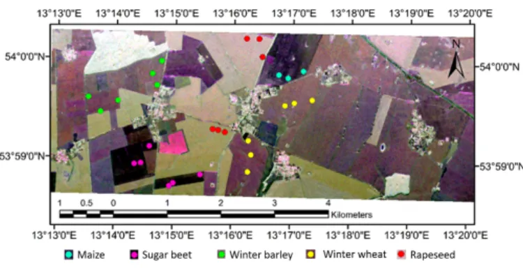
The airborne E-SAR L-band full-pol datasets acquired during the ESA-funded AgriSAR 2006 campaign [32] from April 19 to July 28 are used in this study. The datasets were acquired over the Demmin test site which is located in Western Pomerania, North-East of Germany (53◦45040.4200N,
13◦27049.4500E) as shown in Fig. 1. Major crops grown in this region are: maize, winter wheat, winter barley, rapeseed, and sugar-beet. These crops are generally sown in the first week of April and are harvested by the end of July. According to the AgriSAR2006 campaign report [32], the summer crop calendar is given in Fig. 2. Hence, during the E-SAR data acquisition between June 7 to July 12, most of the crops were in their high vegetative growth stage. Since the objective of this study is to exploit the polarimetric features for classification during the cultivation period (i.e. standing crop condition), the images at the beginning and end of the airborne campaign are not taken into account. Thereby, a total of 5 acquisitions from June 7 to July 12 are used in this study.
Fig. 1. Pauli-RGB image of E-SAR data acquired on June 7 during AgriSAR 2006 campaign along with in-situ sampling locations.
Each flight tracks were around 10 kmlong and3 km wide with the incidence angle varying between 25◦ −55◦. The ground measurements comprising of crop height, biomass,
leaf area index (LAI), soil moisture and surface roughness, were synchronized with the SAR data acquisitions. Of note, these biophysical parameter changes with crop phenological stages. In general, quantitative measures of crop phenology are introduced by assigning a numerical code at the start/end dates of each growth stage according to the BBCH scale (Biologische Bundesanstalt, Bundessortenamt und CHemische Industrie) [33], which ranges from 0 to 99. It refers to the physical changes in the structure or morphology of plant canopy during its phenological development. The temporal variations in the crop height and biomass are shown in Fig. 2 and soil moisture in Fig. 3.
Fig. 2. Crop calendar of DEMMIN test site with crop height and wet biomass during the AgriSAR 2006 campaign.
Fig. 3. Soil moisture variations in different crop fields through the campaign. Sampling data between the vertical blue lines is used in the present study (SB- sugarbeet, RS- rapeseed, WW- winter wheat, WB- winter barley, MZ-maize)
In general, variations in soil moisture on a temporal scale have a significant effect on scattering behaviour from agricul-tural fields. The effect of soil moisture on classification error using L-band E-SAR data acquired during the AgriSAR 2006 campaign is reported in detail in [14]. In the present study, the results have been corroborated by including the influence
of soil moisture as well as vegetation on physical scattering behaviour of crop canopy as discussed in Sec. IV-A.
III. METHODOLOGY
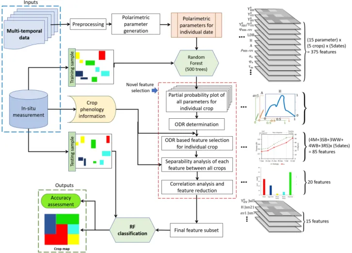
The schematic workflow of the proposed novel feature selection technique for multi-temporal crop classification is given in Fig. 4. The steps involved in the technique are detailed in the following sub-sections.
A. PolSAR image processing
The E-SAR L-band full-polarimetric SAR data were ac-quired in the single-look complex format which is represented in the form of a scattering matrix [S]. The scattering matrix
[S] which is expressed in the backscatter alignment (BSA) convention is expressed in the linear horizontal (H) and linear vertical (V) polarization basis as,
[S] = SHH SHV SV H SV V ⇒ k=V([S]) = 1 2Trace([S]Ψ) (1) where V(·) is the vectorization operator on the scattering matrix and Traceis the sum of the diagonal elements of the matrix. In the monostatic backscattering case, the reciprocity theorem constrains the scattering matrix to be symmetric,i.e.,
SHV = SV H. The corresponding Pauli 2×2 basis matrix
{ΨP} and the target vector,kis given as,
{ΨP}= √ 2 1 0 0 1 √ 2 1 0 0 −1 √ 2 0 1 1 0 (2) k=1 2 SHH+SV V SHH −SV V 2SHV T (3) Similarly, for the Lexicographic basis matrix{ΨL}, the target
vector,Ω is given as, {ΨL}= 2 1 0 0 0 2√2 0 1 0 0 2 0 0 0 1 (4) Ω= SHH √ 2SHV SV V T (5) In general, for Earth observation, targets are complex and produce mixed scattering mechanism. In such a case, the information obtained from the scattering matrix is insufficient to describe the physical properties of the target. So, the second order statistics derived from the scattering matrix in terms of the covariance matrixh[C]ior the coherency matrixh[T]iare used. In the monostatic case, the3×3the coherency and the covariance matrix are generated from the outer product of the associated target vector with its conjugate transpose (Eq. (6) and (7)).
The superscriptT∗ denotes matrix transpose with complex conjugation and h...i denotes a spatial or temporal ensemble average of an imaging window. Subsequently, the orienta-tion angle correcorienta-tion is applied to the coherency matrix [T]
by ”desying” according to Huynen’s terminology [34], [30], which involves rotation of the scattering matrix about the LOS by the angleΨ, and this leads to the roll-invariant scattering matrix.
h[T]i=hk·kT∗i=1 2 h|SHH+SV V|2i h(SHH+SV V)(SHH−SV V)∗i 2h(SHH+SV V)SHV∗ i h(SHH−SV V)(SHH+SV V)∗i h|SHH−SV V|2i 2h(SHH−SV V)SHV∗ i 2hSHV(SHH+SV V)∗i 2hSHV(SHH−SV V)∗i 4h|SHV|2i (6) h[C]i=hΩ·Ω∗Ti= h|SHH|2i √ 2hSHHSHV∗ i hSHHS∗V Vi √ 2hSHVSHH∗ i 2h|SHV|2i √ 2hSHVSV V∗ i hSV VSHH∗ i √ 2hSV VSHV∗ i h|SV V|2i (7)
The multi-temporal images were speckle filtered using the refined Lee filter [35] and were co-registered using ground control points with RMSE < 0.152 m. Subsequently, the speckle-reduced data was subjected to incidence angle(θ) cor-rection using the factor4π/Acosθdue its variation(25◦−55◦)
in range direction [14] andAapproximates to1 m×1 mpixel resolution. This converts the backscattered intensitiesσ0toγ0.
B. Feature set generation
A set of 7 parameters: γ0 HH, γ 0 HV, γ 0 V V, φHH−V V, γ0 HH/γ 0 V V,2γ 0 HV/(γ 0 HH+γ 0
V V), andρHH−V V were derived
from the elements of theh[C]imatrix for an individual date. Subsequently, these parameters were obtained for 5 acquisition dates between June 7 and July 12 thus generating a set of 35 (7×5) parameters. This parameter set was further expanded to 175 features based on the reference data recorded during the in-situ measurement for 5 crops (7×5×5). It has been reported in [1], that the backscatter coefficients (γ0
HH,γHV0 ,γV V0 ) are
positively correlated with vegetation water content. The co-pol phase difference, φHH−V V characterizes the number of
bounces an electromagnetic (EM) wave encounters before it is reflected (scattered) back to the receiver [36]. An ideal odd-bounce would have φHH−V V = 0, whereas an ideal
even-bounce would haveφHH−V V =π.
The correlation coefficient (0≤ |ρHH−V V| ≤1) is one of
the important parameters which characterizes crop phenology. In general, a high correlation between the co-pol channels (|ρHH−V V| ∼1) can be observed at the initial growth stage
of the crop [37]. It is usually characterized by dominating surface scattering from the soil surface. However, the coher-ence between the co-pol channels drops as the stem elongation starts thereby showing an increase in the diffuse scattering component.
The co-pol ratioγ0HH/γV V0 shows significant change during different phenological stages of a crop as it critically depends on its canopy orientation and geometry. In this study, the ratio
2γ0
HV/(γ
0
HH+γ
0
V V) was used as a measure of linear
depo-larization ratio (LDR). In the case of bare soil, the difference between co-pol and cross-pol backscatter intensity is nearly zero, which results in the LDRbeing close to 1. However, as the crop height increases, the cross-pol backscatter intensity increases rapidly compared to the co-pol backscatter resulting in LDR > 1. The inclusion of cross-pol information with co-pol in the LDR was used in [38] for mapping sugarcane growth and the retrieval of its LAI from ENVISAT ASAR dual-pol data.
In addition to the parameters mentioned above, a set of 8 more parameters obtained from the Cloude and Pottier
decomposition [6] and the Touzi decomposition [30] are also used in this study. Both these decomposition theorems are based on the eigenvalue-eigenvector analysis of the h[T]i matrix. In the Cloude-Pottier decomposition, the eigenvalues are utilized to obtain the entropy (H) and the anisotropy (A) parameters. The entropy (H) is a measure of randomness in the scattering process, and it ranges from H = 0 (pure isotropic scatterer) to H = 1(totally random scatterer). The anisotropyAis a measure of target scattering heterogeneity i.e. the relative importance of the second and the third scattering mechanisms. High A indicates the presence of only one dominant secondary scattering process, while lowAindicates the additional contribution of a third scattering process. The scattering type α indicates the scattering mechanism present and it varies from 0 −90◦. The roll-invariant Cloude and Pottier decomposition approach has been widely used for characterization of scattering mechanisms. However, scattering type ambiguities have been reported in [30] for the description of symmetric and asymmetric target scattering.
The Touzi decomposition uses the roll-invariant incoherent scattering model [30]. It introduces a complex quantity αc s
to assess scattering mechanism from symmetric targets. This complex quantity which is represented in polar coordinates
αc
s= (αs,Φαs)is expressed in terms of the con-eigenvalues µ1 andµ2 of[S][30] as,
tan(αs)·ejΦαs =
µ1−µ2
µ1+µ2
(8) where 0 ≤ αs ≤ π/2 and −π/2 ≤ Φαs ≤ π/2. The
symmetric scattering type magnitude and phase (αs,Φαs)
along with the helicity τm is required for an unambiguous
characterization of coherent scattering type [30]. The Cloude Pottier’sα is identical to Touzi’s αs for symmetric scatterer,
i.e., τm = 0. However, for asymmetric scatterer τm 6= 0the
scattering types αand αs provide different information. The
scattering type amplitudeαs= 0 for a pure trihedral whereas
αs=π/2 for a pure dihedral.
The phase difference between the vector components in the trihedral-dihedral basis is given by Φαs. The importance of Φαs can be understood from the fact that only points on the
equator of the Poincar´e sphere can be characterized with αs
if Φαs is neglected. Moreover, two symmetric scatterers at
the equator of the Poincar´e sphere with the same value ofαs
cannot be separated without the knowledge of Φαs.
The use of the target helicityτmpermits separating
symmet-ric from asymmetsymmet-ric scatterers that have the same scattering typeαs[30]. A symmetric target is a target having an axis of
The helicityτmin Touzi decomposition allows the assessment
of the degree of target scattering symmetry. In the literature, the variations in the Touzi decomposition parameters have been analyzed for rice and wheat crop monitoring [39], [40], wetland characterization [41] and snow cover mapping [42]. In the context of this study, the first and the second dominant scattering type αs1, αs2; the first and the second dominant
scattering phase Φαs1 Φαs2; and the first and the second dominant scattering helicity,τm1 andτm2are utilized. Hence, in total 15 polarimetric parameters are used for this study.
C. Random Forest classifier
Random Forest (RF) [23] is an ensemble learning technique which comprises the combination of a large set of indepen-dently generated decision trees. The independence among the trees is attained by randomly selecting a bootstrap sample consisting typically 2/3rd of the data which is used to build each tree. The remaining 1/3rd of the data known as the out-of-bag (OOB) samples are used to obtain an error estimate. At each node of every decision tree, the best split [43] feature is selected from a random subset of features (usually the square root of the total number of features). The mean decrease Gini [27] is one of the standard feature selection techniques in RF. The mean decrease in Gini (MDG) is a measure of the contribution of each variable to the homogeneity of the leaves and nodes of the resulting RF. In addition to MDG, Breiman [23] also proposed a method for feature selection by evaluating the importance of a variable with the Mean Decrease Accuracy (MDA) of the forest. Both of these variable importance measures have shown their practical utility in vari-ous experimental studies. However, these measures are shown to be biased and overestimate the importance of correlated variables [44].
D. Partial Probability Plot
In addition to feature selection, RF uses the partial depen-dence plot [45], [46] which serves as a graphical representation of the marginal effect of a feature on the class probability. The partial dependence function [45] is expressed as,
e f(x) = 1 n n X i=1 f(x, xic) (9)
where x is the feature for which the partial dependence is determined, andxicare the remaining features. The summand
is the logits (log of fraction of votes) for the desired class (10),
f(x) = logpk(x)−
X
j
log pj(X)/K (10)
whereKis the number of classes,pjis the proportion of votes
for classj, andkis the class on which the partial dependence of xis determined.
The partial dependence function is scaled to [0 1] to form the partial probability plots. Therefore, the partial probability plot [47] helps in determining a specific range in which the probability of occurrence of the desired class is high. This particular range also helps in assessing the underlying physical
properties associated with the class. Often, classes may mix due to the similarity in their scattering behaviour. Hence, an optimal range for each feature needs to be identified for which the probability of the presence of the desired class is rather high to separate it from other class labels.
E. Optimal dynamic range (ODR)
The partial probability plot gives the marginal effect of individual parameters on the identification of a crop type. This marginal effect helps to identify the parameters which have a unique range for each crop for a single date. This unique range is termed as the optimal dynamic range (ODR).
In the context of this study, it is important to note that the ODR is not an observable entity. The ODRs are evaluated from the partial probability plots using the training data for each acquisition and for each individual crop. The interpretation of the ODR of a specific polarimetric parameter can be associated with changes in scattering mechanism. The variations in scat-tering mechanisms associated with the phenological growth stages have been incorporated in the present study through the ODR of each polarimetric descriptors. By evaluating the ODR of the same polarimetric parameter for different crops, a parameter subset is created which provides efficient crop separation during classification. Parameters that show similar ODR for two or more crops can be eliminated as these do not supplement the classification accuracy.
In this work, the probability of occurrence of each class for a specific range of each parameter is evaluated. The ODR is conceptualized using Fig. 5. It can be observed that for a probabilityp, a parameter range between B and C is referred to as the ODR. For analysis, the mean ODR (x) corresponding to the probability (p) of occurrence is considered. In the following section (cf. Sec. III-E1), the effect of the ODR as a function of p∈[0.6,1]for a parameter is assessed.
1) ODR Experiment: Following the concept of ODR, it is essential to determine the probability above which two class labels can be significantly discriminated. Hence, an experiment is designed to assess the ideal probability threshold above which the ODR can be appropriately defined. The change in ODR for probability with different ranges are shown in Fig 6. The experiment is performed in two steps:
(a) The LDR and ρHH−V V of July 5 are considered for
a single crop (sugar-beet). The changes in mean ODR for both the parameters were observed as the probability of the presence of sugar-beet class increased from 0.6 to 1. It can be observed from Fig. 6(a), that the mean ODR remained constant for both the parameters forp ≥0.8. For the two parameters, the probability of the presence of a sugar-beet class had the same ODR with a probability of 0.8 beyond which it remains constant. Hence, 0.8 was chosen as the probability threshold to define the ODR.
(b) The ρHH−V V is analyzed to observe the changes in
ODR for two crops (viz., sugar-beet and maize) by increasing
p from 0.6 to 1. It can be observed from Fig. 6(b), that the mean ODR of ρHH−V V is almost similar for both rapeseed
and sugar-beet forp= 0.6 andp = 0.7. At these probabilities, there is a good chance of mixing among these two crop classes
Fig. 4. Schematic workflow of novel feature selection and multi-temporal crop classification using RF.
Fig. 5. Optimal dynamic range (ODR) and mean ODR evaluation.
during classification. However, for a probability of 0.8 and higher, the value of ρHH−V V for both sugar-beet as well
as maize is distinct which results in a successful separation among these two classes. Thus, in this study, 0.8 was set as the ideal probability threshold for ODR determination.
F. Novel feature subset selection technique
A novel feature selection technique is used in this study for multi-temporal crop classification. The feature selection framework is highlighted as follows:
Fig. 6. ODR experiment to determine the ideal probability threshold. (a) Sugar-beet (LDRJuly 5 andρHH−V V July 5); and (b)ρHH−V V July 5
for Sugar-beet and Maize.
• The ODR for each parameter for individual crops were
identified for the multi-temporal dataset. Parameters whose ODR change significantly over the crop pheno-logical stages were selected.
• A particular date in which the features give maximum separation among the crop classes were determined.
• Correlation analysis among the features to remove re-dundancy was performed, and the final feature subset for classification was obtained.
1) Subset selection based on ODR: The partial probability plots for 15 parameters are generated for the training dataset. These plots are made for all the classes separately for each individual date (viz., Entropy for maize, sugar-beet, wheat, barley and rapeseed for June 7). The ODRs for each feature is then determined from their corresponding partial probability plots. Subsequently, the mean ODR for each feature is plotted for all the crops over their phenological stages spanning through the E-SAR acquisition window. However, all the features do not necessarily signify a change in the scattering mechanism w.r.t crop phenology. In fact, depending on the geometrical and dielectric properties of the crop canopy, the parameters may exhibit a different ODR value. Hence, the feature subset comprises of only those parameters whose ODR change significantly with the crop phenology. Among those, 3-4 such parameters are identified for each crop (Fig. 7), e.g., the scattering entropyH andαs1for maize has been selected which shows maximum variations through the growing stages, whereas wheat show relatively minor changes.
Fig. 7. Changes in ODR forαs1andHfor wheat and maize
The changes in scattering mechanism in terms of Cloud’s Entropy and Touzi’s scattering type magnitude αs1 for wheat and maize crops are shown in Fig 7. It can be observed that while there are only minor changes in theH andαs1 param-eters for wheat (Fig 7(a)); maize shows significant changes in their ranges which reflects its diverse scattering characteristics with phenology. It is noticed that the αs1 parameter varies with ∼ 10◦ for wheat, whereas it varies with ∼ 35◦ for maize. Similarly, the Entropy (H) varies with ∼ 0.1 for wheat, whereas it varies with∼0.6for maize throughout their phenological stages. In this study, for each selected parameter, 5 features are obtained for 5 dates viz., αs1 on June 7, June 14, June 21, July 5 and July 12. This feature set is then further refined through the correlation analysis Sec. III-F3.
2) Subset selection based on crop separability analysis:
The disparity in the ODR for each parameter is indicative of the changes in the scattering mechanism due to the crop growth stages. In order to have a reasonable crop classification with low intermixing among the crop classes, the ODR of the chosen parameters is desirable to be different for each crop for a single date. A separability analysis among crops for these selected features are necessary to discriminate phenological stages for classification.
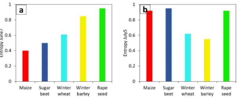
An example of separability assessment is shown in Fig 8. It can be observed that the ODR of H on June 7 shows higher separation among crops compared to the ODR of H
Fig. 8. Separability analysis between crops for two feature (a)Hof June 7 and (b)Hof July 5
on July 5. In particular, the cereal crops (viz., winter wheat and barley) are well separated from others on July 5, but the separation between maize, sugar-beet and rapeseed is poor as compared to June 7. In addition, the ODR of H on June 7 shows separability among maize and sugar-beet in contrast to July 5.
3) Correlation analysis: Besides the selection of a unique subset of features, it is essential to remove redundancy by eliminating the features which show high correlation among them. The correlated features may lead to biased splitting of the node during the tree building process in RF [48]. Hence, in this study, highly correlated features(r >0.5)were eliminated from the feature set. Of note, when correlation between two features is>0.5 e.g.r(A,B)>0.5, then one of them (A or B) has to be eliminated. To select between these two features, the correlation of A and B with other features is checked. If the correlation of either A or B with another feature is∼0.5, then that feature is removed, i.e.,r(A,B)>0.5,r(A,C)<0.5
andr(B,C)∼0.5, then the feature B is removed. It can be observed that the final feature set obtained from the proposed technique is1/25th the size of the initial feature set.
G. RF classification
The RF classification is performed with the novel feature subset obtained from the section mentioned above using 500 trees. At each node of every decision tree, a randomly selected parameter (an approximate square root of a total number of features) were used for node splitting. In this work, 5% of the study area was used to select the training and the testing samples for supervised classification. This is due to the disparate field size of each crop class in the study area. Hence, to avoid classification bias, equal proportions of samples from each class were chosen. In these samples,2/3rd were assigned
for training, and the remaining 1/3rd were used for testing.
The training and the testing samples were selected solely based on the in-situ measurement performed during the AgriSAR 2006 campaign.
The classification accuracies are calculated for each crop class using test samples in terms of producer’s and user’s accuracies (P A and U A respectively). Furthermore, the F1-scores (2×U A×P A/(U A+P A)) are computed for each class. The classification results were also compared with standard feature selection techniques in RF (viz., MDG and MDA) seldom use domain knowledge such as the one associated
with phenology information. It is important to note that, the comparison is not straightforward, as the feature subset obtained from the standard MDA and MDG may include correlated parameters (as discussed in Sec. III-C) which make the variable importance ranking less reliable. Therefore, ap-proximately 15 uncorrelated (r < 0.5) features from top 30 features list of MDA and MDG are selected and subsequently used for classification.
IV. RESULTS AND DISCUSSION
This section explains the results of the novel feature selec-tion technique. The proposed subset selecselec-tion technique was performed using the steps described in subsection A, B and C. A final subset of 15 features obtained from a set of 375 initial features is given in subsection D. In subsection E, the RF classification result using the selected subset is analyzed and subsequently compared with the standard RF feature subset selection techniques (MDA and MDG).
A. Subset selection based on ODR
This section describes the primary feature selection from the multi-temporal PolSAR dataset by utilizing the joint variations in mean ODR of the polarimetric parameter and crop phenol-ogy. Among the 15 polarimetric parameters, 3 or 4 parameters were selected whose ODR showed significant changes with phenology for individual crop. The differences in ODRs of selected parameters are analyzed for maize, sugar-beet, cereal crops and rapeseed in the following subsections.
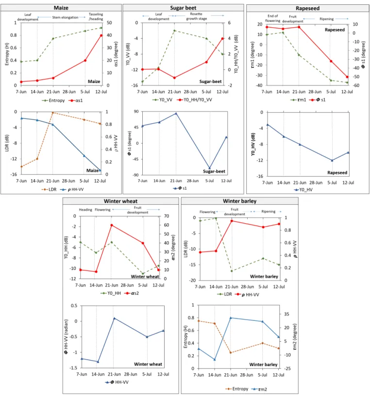
1) Maize: The growth stages of maize between June 7 and July 12 are shown in Fig. 9. During this period, maize advances from leaf development to heading stage. The ODR of αs1,H,LDRandρHH−V V showed considerable changes
with its phenological stages. The αs1 parameter varies from
3◦ to 40◦ whereas H varies from 0.4 to 0.92 during these stages as shown in Fig. 13.
The backscatter response from the exposed soil of the maize fields is responsible for dominant surface scattering mechanism as indicated by low scattering-type magnitudeαs1 andH during the leaf development stage. At the stem elonga-tion stage, though the canopy content (e.g., height, biomass, leaves density, etc.) of maize increases, the surface scattering mechanism from the underlying soil surface is dominant. This is evident from the value ofαs1(∼20◦). However, theH in-creases during this stage which is possibly due to the presence of short stems and leaves. At the heading stage, Scattering goes from surface-dominated (αs1 ∼20◦) to a mixture of surface and volume (αs1∼40◦) withH >0.92. This is evident from a high value of wet biomass (>6.82 kgm−2) and plant height (>110 cm) which causes multiple scattering within the maize canopy.
It is observed in Fig. 13 that the mean ODR ofLDR also varies significantly from−14 dBon June 7 to−4 dBon July 12. During the early stages, the backscatter intensity from the soil is more dominant. This results in the co-pol scattering intensities being similar while the cross-pol scattering intensity is lower than the co-pol. The cross-pol backscatter intensity
increases rapidly as compared to the co-pol backscatter inten-sity, thus leading to an increase of the LDR with the increase of crop biomass and LAI. This also leads to decrease inHH
-V -V correlation from early stage (ρHH−V V = 0.86) to the full
vegetative growth (ρHH−V V = 0.1) of maize canopy.
Fig. 9. Growth Stages of Maize: (a) Leaf development stage (June 7); (b) Stem elongation (June 14); (c) Stem elongation with 3-7 nodes (June 21); (d) Stem elongation with 9 nodes(July 5); (e) Heading or tassel emergence (July 12).
2) Sugar-beet: The ODRs of γ0
V V, γHH0 /γV V0 , and φs1 show significant changes at different growth stages of sugar-beet. The ODR of γV V0 is fairly low (∼−15 dB) during the early leaf development stage, and it increases with increase in biomass and LAI during the rosette growth. However, the sharp increase inγ0
V V (∼9 dB) is observed during the period
from June 14 to June 21. This might be a joint effect of high soil moisture and biomass. The high soil moisture is evident from the reported precipitation events occurred during June 14 to June 21.
The ODR of co-pol ratioγ0
HH/γ
0
V V increases from nearly
0 dBduring the early stage to4 dBin 90% of rosette growth. At the early stage, the γ0
HH and γ
0
V V is nearly similar for
the bare soil surface. However, the sugar-beet canopy grows with laterally spreading broad leaves (planophile) thereby maintaining defined row structures throughout its growing season (Fig. 10). The orientation of the broad planophile leaves of sugar-beet leads to change inγ0
HH andγV V0 . This is evident
from Fig. 13, an increase of co-pol ratio is observed with the plant growth. In addition, scattering type phaseφs1also shows notable variations during different phenological stages. The phase offset of 50◦ between the trihedral and the dihedral scattering is observed during the early stage. However, it approaches ∼ 80◦ during the advanced stages of the plant growth.
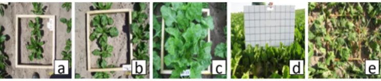
Fig. 10. Growth Stages Sugar-beet. (a) Leaf development 7 leaves unfolded (June 7); (b) 9 and more leaves (June 14); (c) Leaves cover 20% of ground (June 21); (d) Leaves cover 40% of ground (July 5); (e) Leaves cover 90% of ground (July 12).
3) Cereal crop-Wheat and Barley: The phenological stages of wheat and barley are shown in Fig. 11 and 12 respectively. Both these cereal crops have vertically oriented stems and similar crop structure. However, a difference in their growth stages leads to diverse scattering mechanism which is clearly reflected in their varied ODRs.
Fig. 11. Growth Stages Winter Wheat. (a) Inflorescence emergence (June 7); (b) Flowering (June 14); (c) Fruit development started (June 21); (d) Medium milk (July 5); (e) Late milk (July 12).
Fig. 12. Growth Stages Barley. (a) Flowering/anthesis (June 7); (b) Fruit development started with early milk (June 14); (c) Late milk (June 21); (d) Ripening started with early dough (July 5); (e) Fully ripe (July 12).
A noteworthy change is observed in ODRs of γHH0 , αs2,
and the co-pol phase difference, φHH−V V with the growth
stages of wheat as shown in Fig. 13. During this period, the wheat advances from the heading stage (June 7) to a progressive ripening stage (July 12) as shown in Fig. 11. During the heading to the flowering stages, γ0
HH = −5 dB
can be observed for wheat. However, a decrease of4 dBin the ODR ofγ0
HH is seen with the reduction of its biomass during
the ripening stage. Theαs2 also varies from∼8◦ during the inflorescence emergence to∼50◦ during the milking stage of the fruit development.
The ODR of φHH−V V changes from −1.1 radian to
−1.3 radianfrom the full vegetative growth (heading) to the flowering stage. This may be due to the vertical orientation distribution of leaves and stalk of wheat, which causes the changes in the HH andV V phase. However, during the end of the fruit development stage, as the canopy starts drying, theHH and theV V phase difference is approaching close to zero.
Similar to wheat, the ODR of ρHH−V V, LDR, Entropy
(H), and target helicity τm2 show a significant change for barley. These changes in ODR are correlated with the pheno-logical changes during the period of flowering to fully ripening stage (Fig. 12). The ODR of LDR changes from −1 dB to −15 dBas shown in Fig. 13. The cross-pol backscatter inten-sityγ0
HV also decreases significantly for barley as it matures
(or ripens). This change is due to the cross-pol intensity being more sensitive towards the biomass which decreases rapidly from the fruit development to the fully ripening stage (Fig. 2) than the co-pol channel. Thereby, theLDR decreases rapidly during the fruit development to ripening stage.
Besides, as barley dries out, the L-band wave can penetrate the canopy and interact more with underlying soil, that may be the possible cause of the two-fold increase inρHH−V V during
the fruit development stage. Similarly, the ODR of H also changed considerably during the decrease in the biomass from
4.5 kgm−2 at the flowering stage to 1.5 kgm−2 at the fully ripening stage, as the degree of randomness decreases while ripening. The τm2 also shows significant variations during
flowering and fruit development stage. This change may be due to the reduction of the biomass from 4.5 kgm−2 at the flowering stage to1.5 kgm−2 at the fully ripening stage.
The ODR of cross-pol backscatter intensity γHV0 also de-creased from −2 dB to −15 dB for barley as it matures (or ripens). This change is due to the cross-pol intensity being more sensitive towards the biomass which decreases rapidly from the fruit development to the fully ripening stage (Fig. 2).
4) Rapeseed: The phenological stages of rapeseed from June 7 to July 12 is shown in Fig. 14. The ODR ofγ0HV, the Touzi scattering type phaseφs1 and the target helicity show a significant change throughout the growing stages (Fig. 13). A decrease in the cross-pol backscatter intensity (γHV0 ) of9 dB
was observed from the flowering to the end of the ripening stage with a 4 kgm−2 reduction in the biomass. It can be noted that the number of scatterers (viz., pods, leaves, stem) in rapeseed are higher than compared to the other crops which result in a complex scattering phenomenon.
As the pod development begins, the ramified stems and the randomly oriented filled pods create a complex upper canopy structure which increases the multiple scattering phenomena. The changes in the ODR of φs1 from 10◦ to−50◦ indicates the phase shift towards the dominant dihedral type scattering mechanism. The dihedral scattering type may arise due to the interaction of the EM waves with the secondary and tertiary stem pods. Similarly, the target helicity also increases after the development of the pods, as the nature of the target becomes asymmetric.
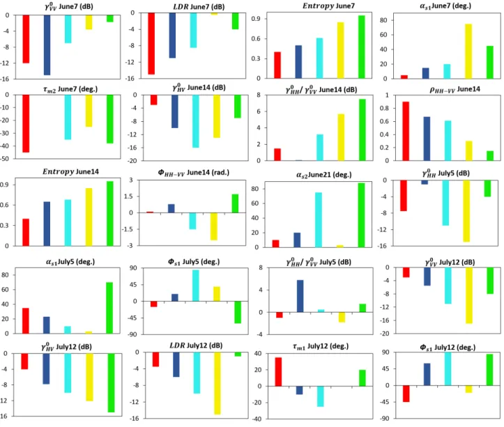
B. Subset selection based on crop separability analysis
A separability analysis was performed on the ODR based feature subset as discussed in section IV-A. The separability analysis plots are shown in Fig. 15. The separability among the crops on a particular date is presented with each of the selected features and discussed below.
The ODR of γ0
V V on June 7 varies from −15 dB to
−1.7 dB. It was observed that while maize and sugar-beet show very low backscatter intensity (−12 dB and−15 dB re-spectively), wheat, barley and rapeseed show high backscatter intensity (>−6.5 dB). This is because, on June 7 maize and sugar-beet are at their initial vegetative growth stages (Fig. 9 and 10) with low biomass. The effect of soil moisture is apparent for maize and sugar-beet as both the crops are at their leaf development stage (with fresh biomass <1.6 kgm−2). However, during this period, the effect of soil moisture is comparatively low in high biomass crop (wheat, barley and rapeseed where fresh biomass>4.2 kgm−2) at the end of their vegetative growth stages (Fig. 11, 12 and 14).
It is observed in Fig. 15 that the LDR, increases with crop height and biomass while it decreases as the soil surface roughness increases. For bare soils, the difference between (γV V0 or γHH0 ) and γHV0 is nearly zero which make the
LDR ∼ 1. As the crop height increases, the cross-pol backscatter intensity (γ0HV) increases rapidly as compared to the co-pol backscatter intensity (γV V0 or γHH0 ), thus leading to an increase of theLDR with the crop biomass [38]. This characteristic was observed in the case of wheat, barley, and
Fig. 13. ODR variations of polarimetric parameters at crop growth stages.
rapeseed on June 7 when they were in their full vegetative growth stages. On the other hand, for maize and sugar-beet, the LDR ∼ −11 dB as these crops are at their early stage with a dominant soil component.
A similar trend is also observed for H and αs1 on June 7 for various crops. A high value of entropy (∼ 0.9) is observed for rapeseed, while it is low (∼0.4) for maize and sugar-beet during their early stage. On the other hand, wheat,
barley, and rapeseed are in the heading and flowering stages which generate more random scattering thereby increasing their entropy (H > 0.6). The αs1 also shows a dominant surface scattering (αs1∼10◦ in maize, sugar-beet and wheat; while it trends towards volume scattering for barley and dihedral type scattering for rapeseed. Also, the target helicity
τm2 varies for different crops as the nature of the different crop target becomes asymmetric.
Fig. 14. Growth Stages Rapeseed. (a) End of flowering (June 7); (b) Fruit development stage (June 14); (c) Beginning of ripening: filling pod (June 21); (d) Beginning of ripening: filling pod (July 5); (e) Nearly fully ripen pods (July 12).
On June 14, maize and sugar beet have an early vegetative stage with low biomass and height (Fig. 2) which should lead to a low cross-pol backscatter response. However, in L-band, the soil contribution is notable for low biomass crops. It is observed in Fig. 15, that γ0
HV responses are −5 dB
and −13 dB for maize and sugar beet. Maize with specific row structure and long stem (during stem elongation stage) generates more cross-pol (HV) backscatter component than sugar beet. In the case of high biomass crops (rapeseed and cereals during the full vegetative stage) the interactions occur between the secondary stems and leaves which causes more attenuation of γ0
HV.
The co-pol ratio,γHH0 /γV V0 on June 14 which depends on the orientation of the crop canopy and its geometry shows a significant change during different phenological stages. For vertical stem crops, like wheat and barley, the high co-pol ratio is possibly due to the vertical orientation of wheat leaves and stalk which bring about different scattering intensities for the HH and theV V polarized waves. On the other hand, the co-pol ratios for the maize and sugar-beet are low since the scattering intensities of theHH andV V polarized waves are similar on June 14. A reverse trend is observed forρHH−V V,
as in low vegetation scenario (maize and sugar-beet) the HH
and the V V are nearly similar. Moreover, the entropy also suggests a low randomness in maize and sugar-beet canopy, while it is high (∼>0.6) for fully grown cereal and rapeseed. On June 14, φHH−V V ∼ 0 for maize and sugar-beet
which suggests an ideal odd-bounce scattering mechanism. This could be due to the penetration of the L-band wave through their low biomass canopy. For wheat, the ODR of
φHH−V V > π/2is due to the depolarization of the EM wave
from the fully vegetative stage on June 14. However, it reaches close to π for rapeseed and wheat which illustrates an even bounce scattering phenomena.
On June 21, the secondary scattering type magnitude αs2 shows various scattering mechanisms respective of low and high biomass crop. A high value of αs2 (>75◦) is observed for high biomass (6.2 kgm−2) crop wheat and rapeseed during their initial fruit development stage. However,αs2 is compar-atively lower (<20◦) for maize, sugar-beet and barley with low biomass.
The ODR ofγHH0 on July 5 varies for different crop types. The backscatter intensity of maize and sugar-beet is −7.5 dB
and−1.5 dBrespectively with a high biomass (>2.5 kgm−2) during their full vegetative growth. However, it is quite low in the matured cereal crops (<−11 dB). Moreover, it is important to note a 5 dB difference in γ0
HH for maize and sugar-beet.
This could be due to the attenuation of theHHintensity in the vertically oriented maize stalks as compared to the horizontal leaf orientation of sugar-beet. In addition, γ0
HH/γV V0 also
shows variations amongst the crops as shown in Fig. 15. The ODR ofαs1 on July 5 varies for different crop types. It is low (∼8◦) for the partially ripened cereal crop while it is high (∼35◦) for the fully vegetative maize and sugar-beet. It indicates surface scattering phenomenon with low biomass cereal crops. However, for the high biomass maize crop, the scattering goes towards a mixture of surface and volume (αs1 ∼ 40◦). For rapeseed crop, the ODR of αs1 ∼ 60◦ represents a more dihedral type scattering mechanism which mostly comes from its complex multiple stems and pods. The similar phenomenon is also evident with the response ofφs1 from various crop types. For maize and sugar-beet the ODR of φs1 ∼ 15◦ is due to the depolarization of the EM wave from the fully vegetative stage. However, it reaches>60◦for rapeseed and wheat which indicates an even bounce scattering phenomena. However, for nearly ripen barley (as compared to wheat) φs1 ∼ 40◦, as in L-band it seems to be transparent with a low biomass (2.7 kgm−2) during the early dough started forming.
The ODR ofγ0
V V on July 12 varies from−17 dBto−3 dB
as shown in Fig. 15. Maize and sugar-beet show a higher backscatter response (−3 dB and−5.5 dBrespectively) than the other crops. This is because, on July 12, maize and sugar-beet are in their full vegetative growth stage while wheat and barley are in their ripening stage (mostly dried out). Hence, wheat and barley have a low V V backscatter on July 12. Among the cereal crops, the V V backscatter from barley is lower as compared to wheat, since barley ripens fully on July 12. The ODR ofγHV0 also shows a similar trend toγV V0 on July 12 as the crop biomass changes.
Theφs1parameter on July 12 shows significant change for all the crops. Maize and sugar-beet in their full vegetative growth generate multiple scattering which shows a phase shift ∼60◦. On July 12, the biomass of barley dries out. This causes an increased wave penetration at L-band resulting in nearly zero phase shift between trihedral and dihedral type scattering. However, the rapeseed with ramified stems and multiple pods may lead to∼90◦ phase shift.
It is observed in Fig. 15 that theLDRof maize and sugar-beet is high (>−6 dB) on July 12 when they were in their full vegetative growth stages. On the other hand, for wheat and barley, the LDR > 10 dB as these crops are partially dried up at the ripening stage. On July 12, as the rapeseed is dried out partially, theHV backscattering is very low∼8dB. However, the co-pol backscattering from the underlying soil surface is significant which makes theLDR∼ −2 dB.
Thus, the selected feature subset obtained from the novel technique is able to discriminate among various crops. This is apparent in the proposed novel feature selection technique which takes into account the changes in the scattering mecha-nism during the crop phenological stages and their subsequent influence on parameters derived from the PolSAR data.
Fig. 15. Separability analysis for feature subset between various crops based on ODR.
C. Subset selection based on correlation analysis
The subset selection after analyzing the changes in the ODR and the crop separability is followed by the correlation analysis amongst the features. From the set of 20 features selected based on crop separability, few were found to be highly correlated as shown in Table I. The features highlighted in bold font in Table I were retained as a part of the final subset. Finally, a set of 15 features (out of 375) are selected for multi-temporal crop classification.
TABLE I CORRELATION ANALYSIS
Features Correlation
γ0
HH/γV V0 June 14&γHH0 /γV V0 July 12 0.526
HJune 14 &HJune 7 0.721
γ0
HH July 5&γ0V V July 12 0.568
φs1July 5 &φs1July 12 0.549
γ0
HV June 14&γHV0 July 12 0.614
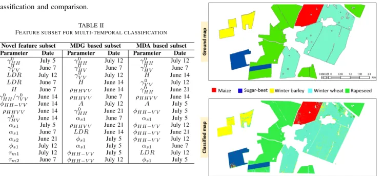
D. Final feature subset selection
The final subset selected using the proposed feature selec-tion technique is given in Table II. For comparison, the MDG and MDA based feature subset are also obtained using the RF. It may be noted that some of the features derived from the proposed technique are identical to the ones obtained by the MDG or MDA.
Furthermore, it is also important to note that half of the features obtained from the proposed technique are different from the ones obtained through the MDG and MDA technique. These include the features based on the eigenvalue-eigenvector based decomposition, H, Touzi decomposition parameters
αs, φs, τmand features based on the ratio of the backscattering
intensities, γ0HH/γV V0 and LDR. Apparently, these features may have provided additional scattering information impor-tant for multi-temporal crop characterization. In addition, the uncorrelated MDA and MDG feature list (as discussed in Sec. III-G) are given in Table II and subsequently used for
classification and comparison. TABLE II
FEATURE SUBSET FOR MULTI-TEMPORAL CLASSIFICATION
Novel feature subset MDG based subset MDA based subset Parameter Date Parameter Date Parameter Date
γ0
HH July 5 γHH0 July 12 γHH0 July 12
γ0
V V June 7 γ0HV June 7 γ0HV June 7
LDR July 12 γ0
V V July 12 H June 14
LDR June 7 H June 14 γ0
V V July 12
H June 7 ρHHV V June 14 γHH0 June 21
γ0
HH/γV V0 June 14 ρHHV V June 7 ρHHV V June 14
φHH−V V June 14 A July 12 A July 5
ρHHV V June 14 γHH0 June 21 φHH−V V July 5
γ0
HV June 14 αs1 June 7 αs1 July 5 αs1 July 5 ρHHV V June 21 φHH−V V July 12
αs1 June 7 LDR June 14 φHH−V V June 21
αs2 June 21 φs1 July 5 φHH−V V July 12
φs1 July 12 αs1 July 5 αs1 June 7 τm1 July 12 φHH−V V July 5 LDR July 12
τm2 June 7 φHH−V V July 12 φs1 July 5
E. Classification results
A multi-temporal RF crop classification shown in Fig. 16 was performed using the feature subset obtained from the proposed technique. A crop inventory map from AgriSAR 2006 campaign was used for accuracy assessment of classified output Map. The overall accuracy (OA) achieved using the phenology-based multi-temporal feature selection technique is 99.12% with a kappa coefficient (κ) of 0.99. The producer’s accuracy (PA) and the user’s accuracy (UA) are shown in Table III. The PA and UA for all the crops are > 98.5%
for all the crops except for barley (PA ≈ 89.68%). It can be observed that 10.32% of the barley test pixels are mixed with wheat which has similar phenological stages. In addition, the F1 score which is the weighted average of the PA and UA describes the accuracy of classification, especially with an uneven class distribution. The F1 score is >99%for most of the crops using the phenology-based feature selection method. However, the F1 score of barley is comparatively low (94.56). The classification accuracy using the novel feature subset was nominally better than the standard MDG and MDA methods. The proposed feature selection technique which incorporated the domain knowledge in the form of the phenol-ogy information associated with the temporal dataset yielded competent classification results. It provided a rationale by relating the feature subset to the underlying physical properties associated with the crop class.
V. SUMMARY ANDCONCLUSION
Standard feature selection techniques seldom incorporate domain knowledge associated with the physical properties of the targets. Hence, a novel feature selection technique was proposed in this study for multi-temporal crop classification. This technique takes into account the changes in the scattering mechanism during the crop phenological stages and their subsequent influence on parameters estimated from PolSAR data.
The proposed feature selection technique was performed using three major steps: (a) The marginal effect of the features
Fig. 16. Multi-temporal crop classification using RF along with ground map.
on a class was identified using the RF-based partial probability plot. The optimal dynamic range (ODR) of each parameter for individual crops were determined. Subsequently, three-four such parameters were chosen for each crop. (b) A feature subset was chosen which provides ample separation of the ODR for different crops on the same date. (c) Finally, few highly correlated features (>0.5) were removed from the final subset.
The multi-temporal crop classification accuracy using this novel feature selection technique was 99.12%. The classifi-cation accuracy using the proposed technique was nominally better than the standard feature selection technique used in RF (MDA and MDG). The novel subset generated in this study seems to be more reliable than the subset obtained by standard RF methods viz., MDA and MDG since it only includes highly uncorrelated features. It was reported in previous studies that the standard variable importance measures used in RF are not reliable in the presence of highly correlated parameters, such as the ones included in this study. Also, it is important to note that the MDA and the MDG technique do not take into account any domain knowledge associated with crop phenology. In fact, the phenology information is essential for crop characterization and classification as analyzed in this study. It can be concluded that the target decomposition parameters and the ratio of the backscattering intensities which effectively incorporate phenological information were vital for multi-temporal crop classification in this study.
It is suggested that for feature selection studies in the future, the domain knowledge be incorporated in some form. Also, it is advisable to use novel feature selection techniques which incorporate physical scattering mechanism and may provide improved classification accuracy with an insight of the physical properties associated with the class. The novel feature selection technique introduced in this study can be useful for studies which involve multi-temporal datasets. The proposed
TABLE III
CLASSIFICATION ACCURACY USING DIFFERENT FEATURE SELECTION TECHNIQUES Crop Novel feature based MDG based MDA based
PA UA F1 Score PA UA F1 Score PA UA F1 Score Maize 100 99.05 99.52 99.88 92.16 95.86 99.76 91.65 95.53 Sugar beet 98.82 100 99.41 89.53 99.84 94.40 88.20 99.50 93.51 Winter wheat 99.98 98.53 99.25 99.56 99.59 99.57 99.75 99.41 99.58 Winter barley 89.68 100 94.56 96.83 97.29 97.06 96.35 98.70 97.51 Rapeseed 99.67 99.97 99.82 99.67 99.87 99.77 99.67 99.90 99.78 κ 0.99 0.98 0.98 OA 99.12 98.73 98.68
feature selection has potential applications in the field of snow phenology and land surface phenology monitoring.
ACKNOWLEDGMENT
The authors would like to thank the European Space Agency (ESA) and the German Aerospace Center (DLR) for providing the AgriSAR 2006 campaign data through Project ID: 34188.
REFERENCES
[1] H. McNairn and J. Shang, “A review of multitemporal synthetic aperture radar (SAR) for crop monitoring,” inMultitemporal Remote Sensing. Springer, 2016, pp. 317–340.
[2] K. Chen, W. Huang, D. Tsay, and F. Amar, “Classification of multi-frequency polarimetric SAR imagery using a dynamic learning neural network,”IEEE Trans. Geosci. Remote Sens., vol. 34, no. 3, pp. 814– 820, 1996.
[3] D. H. Hoekman and M. A. Vissers, “A new polarimetric classification approach evaluated for agricultural crops,”IEEE Trans. Geosci. Remote Sens., vol. 41, no. 12, pp. 2881–2889, 2003.
[4] H. Skriver, “Crop classification by multitemporal C-and L-band single-and dual-polarization single-and fully polarimetric SAR,”IEEE Trans. Geosci. Remote Sens., vol. 50, no. 6, pp. 2138–2149, 2012.
[5] C. P. Tan, H. T. Ewe, and H. T. Chuah, “Agricultural crop-type classification of multi-polarization SAR images using a hybrid entropy decomposition and support vector machine technique,”Int. J. Remote Sens., vol. 32, no. 22, pp. 7057–7071, 2011.
[6] S. R. Cloude and E. Pottier, “An entropy based classification scheme for land applications of polarimetric SAR,”IEEE Trans. Geosci. Remote Sens., vol. 35, no. 1, pp. 68–78, 1997.
[7] H. McNairn, A. Kross, D. Lapen, R. Caves, and J. Shang, “Early season monitoring of corn and soybeans with TerraSAR-X and RADARSAT-2,”
Int. J. Appl. Earth Observ. Geoinf, vol. 28, pp. 252–259, 2014. [8] Z. Qi, A. G.-O. Yeh, X. Li, and Z. Lin, “A novel algorithm for land
use and land cover classification using RADARSAT-2 polarimetric SAR data,”Remote Sens. Environ., vol. 118, pp. 21–39, 2012.
[9] Z. Yang, K. Li, L. Liu, Y. Shao, B. Brisco, and W. Li, “Rice growth monitoring using simulated compact polarimetric C-band SAR,”Radio Sci., vol. 49, no. 12, pp. 1300–1315, 2014.
[10] S. C. Steele-Dunne, H. McNairn, A. Monsivais-Huertero, J. Judge, P.-W. Liu, and K. Papathanassiou, “Radar remote sensing of agricultural canopies: A review,”IEEE J. Sel. Topics Appl. Earth Observ. Remote Sens., vol. 10, no. 5, pp. 2249–2273, 2017.
[11] J. M. Lopez-Sanchez, F. Vicente-Guijalba, J. D. Ballester-Berman, and S. R. Cloude, “Polarimetric response of rice fields at C-band: Analysis and phenology retrieval,”IEEE Trans. Geosci. Remote Sens., vol. 52, no. 5, pp. 2977–2993, 2014.
[12] X. Jiao, J. M. Kovacs, J. Shang, H. McNairn, D. Walters, B. Ma, and X. Geng, “Object-oriented crop mapping and monitoring using multi-temporal polarimetric RADARSAT-2 data,”ISPRS J. Photogramm. Remote Sens., vol. 96, pp. 38–46, 2014.
[13] X. Huang, J. Wang, J. Shang, C. Liao, and J. Liu, “Application of polarization signature to land cover scattering mechanism analysis and classification using multi-temporal C-band polarimetric RADARSAT-2 imagery,”Remote Sens. Environ., vol. 193, pp. 11–28, 2017.
[14] H. Skriver, F. Mattia, G. Satalino, A. Balenzano, V. R. Pauwels, N. E. Verhoest, and M. Davidson, “Crop classification using short-revisit multitemporal SAR data,” IEEE J. Sel. Topics Appl. Earth Observ. Remote Sens., vol. 4, no. 2, pp. 423–431, 2011.
[15] H. McNairn, J. Shang, C. Champagne, and X. Jiao, “TerraSAR-X and RADARSAT-2 for crop classification and acreage estimation,” in
Geoscience and Remote Sensing Symposium, 2009 IEEE International, IGARSS 2009, vol. 2. IEEE, 2009, pp. II–898.
[16] D. Bargiel and S. Herrmann, “Multi-temporal land-cover classification of agricultural areas in two european regions with high resolution spotlight TerraSAR-X data,”Remote Sens., vol. 3, no. 5, pp. 859–877, 2011. [17] R. Sonobe, H. Tani, X. Wang, N. Kobayashi, and H. Shimamura,
“Discrimination of crop types with TerraSAR-X-derived information,”
Physics and Chemistry of the Earth, Parts A/B/C, vol. 83, pp. 2–13, 2015.
[18] L. Loosvelt, J. Peters, H. Skriver, B. De Baets, and N. E. Verhoest, “Impact of reducing polarimetric SAR input on the uncertainty of crop classifications based on the random forests algorithm,” IEEE Trans. Geosci. Remote Sens., vol. 50, no. 10, pp. 4185–4200, 2012. [19] A. L. Blum and P. Langley, “Selection of relevant features and examples
in machine learning,”Artificial intelligence, vol. 97, no. 1, pp. 245–271, 1997.
[20] S. Siachalou, G. Mallinis, and M. Tsakiri-Strati, “A hidden markov models approach for crop classification: Linking crop phenology to time series of multi-sensor remote sensing data,”Remote Sens., vol. 7, no. 4, pp. 3633–3650, 2015.
[21] B. Kenduiywoa, D. Bargiel, and U. Soergel, “Spatial-temporal condi-tional random fields crop classification from Terrasar-X images,”ISPRS Annals of the Photogrammetry, Remote Sensing and Spatial Information Sciences, vol. 2, no. 3, p. 79, 2015.
[22] D. Bargiel, “A new method for crop classification combining time series of radar images and crop phenology information,”Remote Sens. Environ., vol. 198, pp. 369–383, 2017.
[23] L. Breiman, “Random forests,”Machine learning, vol. 45, no. 1, pp. 5–32, 2001.
[24] M. Pal, “Random forest classifier for remote sensing classification,”Int. J. Remote Sens., vol. 26, no. 1, pp. 217–222, 2005.
[25] A. O. Ok, O. Akar, and O. Gungor, “Evaluation of random forest method for agricultural crop classification,”European Journal of Remote Sensing, vol. 45, no. 3, p. 421, 2012.
[26] R. Sonobe, H. Tani, X. Wang, N. Kobayashi, and H. Shimamura, “Ran-dom forest classification of crop type using multi-temporal TerraSAR-X dual-polarimetric data,”Remote Sens. Lett., vol. 5, no. 2, pp. 157–164, 2014.
[27] K. J. Archer and R. V. Kimes, “Empirical characterization of random forest variable importance measures,”Computational Statistics & Data Analysis, vol. 52, no. 4, pp. 2249–2260, 2008.
[28] C. Strobl and A. Zeileis, “Danger: High power! ? exploring the statistical properties of a test for random forest variable importance,” 2008. [Online]. Available: http://nbn-resolving.de/urn/resolver.pl?urn=nbn:de: bvb:19-epub-2111-8
[29] K. K. Nicodemus and J. D. Malley, “Predictor correlation impacts machine learning algorithms: implications for genomic studies,” Bioin-formatics, vol. 25, no. 15, pp. 1884–1890, 2009.
[30] R. Touzi, “Target scattering decomposition in terms of roll-invariant target parameters,”IEEE Trans. Geosci. Remote Sens., vol. 45, no. 1, pp. 73–84, 2007.
[31] S. Hariharan, S. Tirodkar, and A. Bhattacharya, “Polarimetric SAR decomposition parameter subset selection and their optimal dynamic range evaluation for urban area classification using random forest,”Int. J. Appl. Earth Observ. Geoinf, vol. 44, pp. 144–158, 2016.
[32] R. Bianchi, M. Davidson, I. Hajnsek, M. Wooding, and C. Wloczyk, “AgriSAR 2006–final report,” 2008.
[33] H. Bleiholder, E. Weber, P. Lancashire, C. Feller, L. Buhr, M. Hess, H. Wicke, H. Hack, U. Meier, R. Klose et al., “Growth stages of mono-and dicotyledonous plants, BBCH monograph,”Federal
Biologi-cal Research Centre for Agriculture and Forestry, Berlin/Braunschweig, Germany, p. 158, 2001.
[34] J.-S. Lee, D. L. Schuler, and T. L. Ainsworth, “Polarimetric SAR data compensation for terrain azimuth slope variation,”IEEE Trans. Geosci. Remote Sens., vol. 38, no. 5, pp. 2153–2163, 2000.
[35] J.-S. Lee, J.-H. Wen, T. L. Ainsworth, K.-S. Chen, and A. J. Chen, “Improved sigma filter for speckle filtering of SAR imagery,” IEEE Trans. Geosci. Remote Sens., vol. 47, no. 1, pp. 202–213, 2009. [36] G. Satalino, F. Mattia, T. Le Toan, and M. Rinaldi, “Wheat crop mapping
by using ASAR AP data,”IEEE Trans. Geosci. Remote Sens., vol. 47, no. 2, pp. 527–530, 2009.
[37] J. M. Lopez-Sanchez, S. R. Cloude, and J. D. Ballester-Berman, “Rice phenology monitoring by means of SAR polarimetry at X-band,”IEEE Trans. Geosci. Remote Sens., vol. 50, no. 7, pp. 2695–2709, 2012. [38] H. Lin, J. Chen, Z. Pei, S. Zhang, and X. Hu, “Monitoring sugarcane
growth using ENVISAT ASAR data,”IEEE Trans. Geosci. Remote Sens., vol. 47, no. 8, pp. 2572–2580, 2009.
[39] K. Li, B. Brisco, S. Yun, and R. Touzi, “Polarimetric decomposition with RADARSAT-2 for rice mapping and monitoring,”Can. J. Remote Sens., vol. 38, no. 2, pp. 169–179, 2012.
[40] S. Kar, D. Mandal, A. Bhattacharya, and J. Adinarayana, “Temporal analysis of touzi parameters for wheat crop characterization using l-band agrisar 2006 data,” inGeoscience and Remote Sensing Symposium (IGARSS), 2017 IEEE International. IEEE, 2017, pp. 3909–3912. [41] R. Touzi, A. Deschamps, and G. Rother, “Phase of target scattering for
wetland characterization using polarimetric C-band SAR,”IEEE Trans. Geosci. Remote Sens., vol. 47, no. 9, pp. 3241–3261, 2009.
[42] A. Muhuri, S. Manickam, and A. Bhattacharya, “Scattering mechanism based snow cover mapping using RADARSAT-2 C-Band polarimetric SAR data,” IEEE J. Sel. Topics Appl. Earth Observ. Remote Sens., vol. 10, no. 7, pp. 3213–3224, July 2017.
[43] A. Liaw and M. Wiener, “Classification and regression by randomforest,”
R news, vol. 2, no. 3, pp. 18–22, 2002.
[44] C. Strobl, A.-L. Boulesteix, T. Kneib, T. Augustin, and A. Zeileis, “Con-ditional variable importance for random forests,”BMC bioinformatics, vol. 9, no. 1, p. 307, 2008.
[45] J. H. Friedman, “Greedy function approximation: A gradient boosting machine,”The Annals of Statistics, vol. 29, no. 5, pp. pp. 1189–1232, 2001.
[46] T. Hastie, R. Tibshirani, J. Friedman, and J. Franklin, “The elements of statistical learning: data mining, inference and prediction,” The Mathematical Intelligencer, vol. 27, no. 2, pp. 83–85, 2005.
[47] R Core Team, R: A Language and Environment for Statistical Computing, R Foundation for Statistical Computing, Vienna, Austria, 2013, ISBN 3-900051-07-0. [Online]. Available: http://www.R-project. org/
[48] B. Gregorutti, B. Michel, and P. Saint-Pierre, “Correlation and variable importance in random forests,”Statistics and Computing, vol. 27, no. 3, pp. 659–678, 2017.
Siddharth Hariharanreceived his Bachelor of En-gineering (B.E) degree in electronics and telecom-munications from the University of Mumbai, Mum-bai, India in 2007. He completed his M.Tech in geoinformatics and natural resources engineering and Ph.D. degree from the Centre of Studies in Re-sources Engineering (CSRE) at IIT Bombay, Mum-bai, India, in 2010 and 2018 respectively.
Dr. Siddharth is currently an institute research associate at CSRE, IIT Bombay. He has worked in the field of geoinformatics over the last decade, with particular attention in the domain of satellite image processing and microwave remote sensing using polarimetric SAR datasets. He has contributed novel research for Earth Observation applications in the field of urban area clas-sification, crop classification and mineral prospectivity mapping during his doctoral work.
Dipankar Mandal(S’16) received the B.Tech. de-gree in agricultural engineering from Bidhan Chan-dra Krishi Viswsavidyalaya, Mohanpur, West Ben-gal, India in 2015. He is currently working toward the M.Tech + Ph.D. dual degree in SAR remote sensing in the Indian Institute of Technology Bom-bay, Mumbai, India. His research interest includes applications of SAR polarimetry for crop classifi-cation, vegetation biophysical parameter estimation and yield forecasting.
Siddhesh Tirodkar received his B.E. equivalent AMAeSI (Associate Member of Aeronautical Soci-ety of India) degree in aeronautical engineering from the AeSI, New Delhi, India in 2013. He completed his M.Tech in Mechanical Engineering from the University of Mumbai, Mumbai, India in 2016.
He is currently pursuing his PhD from the Indian Institute of Technology Bombay, Mumbai, India in Climate Studies which is an Interdisciplinary pro-gramme (IDP), since 2016. His research interests include a wide variety of applications in the field of remote sensing, image processing, machine learning, numerical and predictive modelling. He has also worked in the domain of geophysical flows, ocean modelling and mineral prospectivity mapping.
Vineet Kumar(S’15) received the B.Tech. degree in electronics and communication engineering from Uttar Pradesh Technical University, Lucknow, India, in 2010, and the M.Tech. degree in remote sens-ing and GIS from the Indian Institute of Remote Sensing, Dehradun, Uttarakhand, India, in 2013, and JEP with Andhra University, Vishakhapatnam, India. He is currently working toward the Ph.D. degree in SAR remote sensing in the Indian Institute of Technology Bombay, Mumbai, India. His research interest includes applications of Full and Compact SAR polarimetry, for classification and characterization of vegetaion, and relating biophysical variables of crops to SAR observables.
Mr. Kumar received the Shastri Research Student Fellowship 2016 Award by the Shastri Indo-Canadian Research Institute, India and served as a visiting researcher to Carleton Univeristy, Ottawa and Agriculture and Agri-Food, Ottawa, Canada from April to July 2016.