Algorithms and Dynamic Data Structures for
Basic Graph Optimization Problems
by Ran Duan
A dissertation submitted in partial fulfillment of the requirements for the degree of
Doctor of Philosophy
(Computer Science and Engineering) in The University of Michigan
2011
Doctoral Committee:
Assistant Professor Seth Pettie, Chair Professor Anna C. Gilbert
Professor Quentin F. Stout
TABLE OF CONTENTS
LIST OF FIGURES . . . v
ABSTRACT . . . vii
CHAPTER I. Introduction . . . 1
1.1 Basic Concepts and Notations . . . 2
1.2 Overview of the Results . . . 3
1.2.1 Shortest Path and Bottleneck Path . . . 3
1.2.2 Dynamic Connectivity . . . 7
1.2.3 Matching . . . 9
1.3 Publications Arising from this Thesis . . . 11
II. Approximate Maximum Weighted Matching in Linear Time 12 2.1 Introduction . . . 12
2.2 Definitions and Preliminaries . . . 13
2.3 Weighted Matching and Its LP Formulation . . . 14
2.4 A Scaling Algorithm for Approximate MWM . . . 18
2.4.1 The Scaling Algorithm . . . 20
2.4.2 Analysis and Correctness . . . 23
2.4.3 A Linear Time Algorithm . . . 27
2.4.4 Conclusion . . . 31
III. Connectivity Oracle for Failure-Prone Graphs . . . 32
3.1 The Euler Tour Structure . . . 33
3.2 Constructing the High-Degree Hierarchy . . . 37
3.2.1 Definitions . . . 37
3.2.2 The Hierarchy Tree and Its Properties . . . 38
3.3 Inside the Hierarchy Tree . . . 44
3.4 Recovery From Failures . . . 52
3.4.1 Deleting Failed Vertices . . . 52
3.4.2 Answering a Connectivity Query . . . 54
3.5 Conclusion . . . 56
IV. All-Pair Bottleneck Paths and Bottleneck Shortest Paths . . 57
4.1 Definitions . . . 58
4.1.1 Row-Balancing and Column-Balancing . . . 58
4.1.2 Matrix Products . . . 59
4.2 Dominance and APBP . . . 60
4.2.1 Max-Min Product . . . 62
4.2.2 Explicit Maximum Bottleneck Paths . . . 64
4.3 Bottleneck Shortest Paths . . . 65
4.3.1 Rectangular Matrix Multiplication . . . 66
4.3.2 Hybrid Products . . . 66
4.3.3 APBSP with Edge Capacities . . . 71
4.3.4 APBSP with Vertex Capacities . . . 72
V. Dual-Failure Distance Oracle . . . 75
5.1 Introduction . . . 75
5.2 Notations: . . . 77
5.3 Review of the One-Failure Distance Oracle . . . 78
5.3.1 Structure . . . 78
5.3.2 Query Algorithm . . . 79
5.4 Case I . . . 80
5.4.1 Structures . . . 80
5.4.2 The detour from x toy avoiding u . . . 83
5.5 Case II: One failed vertex on xy . . . 88
5.5.1 Data Structures . . . 89
5.5.2 Query Algorithm . . . 92
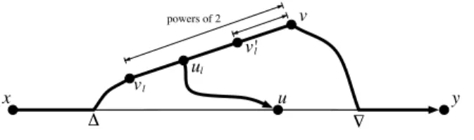
5.6 Case III: Two failed vertices on xy . . . 100
5.6.1 If|xu| or |vy| is a power of 2 . . . 100
5.6.2 The binary partition structure . . . 100
5.6.3 General Cases . . . 104
VI. Dynamic Subgraph Connectivity Oracles . . . 108
6.1 Basic Structures . . . 109
6.1.1 Euler Tour List . . . 109
6.1.2 Adjacency Graph . . . 110
6.1.3 ET-list for adjacency . . . 111 6.2 Dynamic Subgraph Connectivity with Sublinear Worst-case
6.2.1 The structure . . . 113
6.2.2 Switching a vertex . . . 117
6.2.3 Answering a query . . . 120
6.3 Dynamic Subgraph Connectivity with ˜O(m2/3) Amortized Up-date Time and Linear Space . . . 121
VII. All-Pair Bounded-Leg Shortest Paths . . . 125
7.1 The notations . . . 125
7.2 A Binary Partition Algorithm . . . 128
7.3 Answer a bounded-leg shortest path query . . . 131
7.4 A one-level algorithm for all-pair bounded-leg distance . . . . 132
LIST OF FIGURES
Figure
2.1 Illustration of blossom hierarchy and augmentation on it . . . 16
2.2 The Scaling Algorithm . . . 22
3.1 The Euler Tour structure . . . 36
3.2 The construction of the Hierarchy Tree . . . 39
3.3 The structure inside the Hierarchy Tree . . . 46
3.4 The construction of the Euler Tour structure C(T) . . . 50
5.1 One-failure structure . . . 80
5.2 The tree structure . . . 83
5.3 The usage of tree structure in Case I.1.b. . . 86
5.4 Illustration of Case I.2.a . . . 87
5.5 Illustration of Case I.2.a(3) . . . 88
5.6 Illustration of the position ofu0 and cbl, etc. . . . 90
5.7 Illustration of F and F0 . . . . 92
5.8 Illustration of Subcases 1 and 2 . . . 95
5.9 Illustration of Case II.2 . . . 98
5.11 A path in Case III . . . 103
5.12 The illustration of the positions of u, L and m. . . 105
5.13 The fourth type in Case III . . . 106
6.1 Two types of Euler Tour structures . . . 112
7.1 Modified Floyd Algorithm . . . 128
ABSTRACT
Algorithms and Dynamic Data Structures for Basic Graph Optimization Problems by
Ran Duan
Chair: Seth Pettie
Graph optimization plays an important role in a wide range of areas such as com-puter graphics, computational biology, networking applications and machine learning. Among numerous graph optimization problems, some basic problems, such as shortest paths, minimum spanning tree, and maximum matching, are the most fundamental ones. They have practical applications in various fields, and are also building blocks of many other algorithms. Improvements in algorithms for these problems can thus have a great impact both in practice and in theory.
In this thesis, we study a number of graph optimization problems. The results are mostly about approximation algorithms solving graph problems, or efficient dynamic data structures which can answer graph queries when a number of changes occur. There are several different models of dynamic graphs. Much of my work focuses on
the dynamic subgraph model in which there is a fixed underlying graph and every
vertex can be flipped “on” or “off”. The queries are based on the subgraph induced by the “on” vertices. Our results make significant improvements to the previous algorithms or structures of these problems.
• Approximate Matching. We give the first linear time algorithm for computing approximate maximum weighted matching for arbitrarily small approximation ratio.
• d-failure Connectivity Oracle. For an undirected graph, we give the first
space-efficient data structure that can answer connectivity queries between any pair of vertices avoiding d other failed vertices in time polynomial indlogn.
• (Max, Min)-Matrix Multiplication We give a faster algorithm for the (max,
min)-matrix multiplication problem, which has a direct application to the all-pairs bottleneck paths (APBP) problem. Given a directed graph with a capacity on each edge, the APBP problem is to determine, for all pairs of vertices s and t, the path from s to t with maximum flow.
• Dual-failure Distance Oracle. For a given directed graph, we construct a data
structure of size ˜O(n2) which can efficiently answer distance and shortest path
queries in the presence of two node or link failures.
• Dynamic Subgraph Connectivity. We give the first subgraph connectivity
struc-ture with worst-case sublinear time bounds for both updates and queries.
• Bounded-leg Shortest Path. In a weighted, directed graph anL-bounded leg path
is one whose constituent edges have length at mostL. We give an algorithm for preprocessing a directed graph in ˜O(n3) time in order to answer approximate
bounded leg distance and bounded leg shortest path queries in merely sub-logarithmic time.
CHAPTER I
Introduction
This thesis studies several graph optimization problems. Graph optimization plays an important role in a wide range of areas such as computer graphics, computational biology, networking applications and machine learning. Among numerous graph opti-mization problems, some basic problems, such as shortest paths, minimum spanning tree, and maximum matching, are the most fundamental ones. They have practical applications in various fields, and are also building blocks of many other algorithms. Much of my research concerns computing shortest paths and maximum matching. The shortest path problem is essential in web mapping and network routing appli-cations, while the maximum matching problem has applications to assignment prob-lems. They are also important in solving other graph optimization problems like the min-cost maximum flow problem or edge disjoint paths problem. Improvements in algorithms for these problems can thus have a great impact both in practice and in theory.
As we see in the example of web mapping applications, the maps in real world are vulnerable to changes caused by traffic congestions, road failures, or construction of new roads. Instead of re-computing all the information when a change occurs, we may keep as much information of the previous graph as possible in order to improve the running time. A common way to deal with this is building data structures on such
dynamic graphs, which have fast algorithms for updating the structure and answering queries about some graph optimization problem. The running times for updates and queries are usually faster than the original static algorithm on the same problem.
In this thesis we study different variations of several basic graph optimization problems, including bounded-leg shortest paths, data structures maintaining short-est paths or connectivity for failure-prone graphs, worst-case dynamic structure for connectivity, and also algorithms to find all-pair bottleneck paths and approximate maximum weighted matching.
1.1
Basic Concepts and Notations
In this thesis, we denote the primary graph we are working on by G = (V, E), whereV is the set of vertices andE is the set of edges inG. Letn =|V|andm=|E|. The graph can be directed or undirected. Apath pis a sequence of consecutive edges. In a graph with weight function w : E → R on edges, the shortest path problem considers the path minimizingP
e∈pw(e) between two vertices, while the connectivity problem only considers whether there is a path connecting two vertices. In this thesis, all the connectivity problems are in undirected graphs, whereas shortest paths and bottleneck paths are in directed graphs.
A matching M in a graph G is a set of edges without common vertices. A
ver-tex associated with an edge in the matching is called matched, otherwise it is
un-matched. A matching in which all vertices are matched is called a perfect matching.
In a weighted graph, the maximum weighted matching is the matching maximizing
P
e∈Mw(e). Note that it is not necessarily perfect.
Usually there are several types of dynamic graph models. In a fully dynamic
model we can add or delete edges/vertices arbitrarily. There are also incremental
and decremental graphs in which we can only insert or delete edges/vertices,
subgraph model in which there is a fixed underlying graph, and every vertex in that graph can be “active” or “inactive”. The distance/connectivity queries are based on the subgraph induced by the active vertices. We also study two types of this model based on whether there is a restriction on the number of inactive vertices. The structures in Chapter VI do not have such a restriction, that is, any vertex can change its status at any time. However, the results in Chapter III and V consider the dynamic subgraph model in which the number of inactive vertices is bounded by some number d. We can see this type of structure as static, which can preprocess the entire graph and answer the distance/connectivity queries given with several “failed” vertices. This is the “d-failure model”. In the connectivity structure of Chapter III, d can be an arbitrary integer, while in the shortest path structure of Chapter V,d is at most 2.
In this paper, ˜O(·) hides poly-logarithmic factors. For example O(n1/2logn) can
be written as ˜O(n1/2).
1.2
Overview of the Results
1.2.1 Shortest Path and Bottleneck Path
The all-pair shortest path problem is one of the most fundamental and most studied optimization problems in graph theory. It can be solved by applying the Dijkstra’s algorithm from every vertex in the graph, which has a total running time of O(mn+n2logn). (See [17].) A faster running time of O(mn+n2log logn) was
achieved by Pettie [50]. For dense graphs, the Floyd-Warshall algorithm [13] provides a clearer way to achieve the time bound ofO(n3). We can also see the all-pair shortest
path problem as the transitive closure of the (min,+) matrix product. However, since (min,+) is not a ring, the fast matrix multiplication algorithms like [12] cannot be directly applied to it. However, Shoshan and Zwick [58, 69] gave algorithms ofo(n3)
running time for computing all-pair shortest paths in unweighted or small integer weighted graphs by fast matrix multiplication. The current best algorithm for real-weighted graph is given by Chan [9], which has a running time of aboutO(n3/log2n).
In this thesis, we consider several variations of the all-pair shortest path problem: dynamic shortest path, bounded-leg shortest path and all-pair bottleneck path, which are discussed in the following.
1.2.1.1 Dual-failure Shortest Path Structure
In this problem we consider a data structure answering distance queries in a weighted directed graph G = (V, E, w), where one or more nodes or edges are un-available due to failure or other causes. Specifically, given source and target vertices x, y and a set F ⊂V, the problem is to report δG−F(x, y), where δG0 is the distance
function w.r.t. a subgraph G0 of G. In the absence of failure, the best oracle for answering distance queries in O(1) time is a trivial n×n lookup table. Thus, a dis-tance oracle that is sensitive to node failures should be considered (nearly) optimal if it occupies (nearly) quadratic space and answers queries in (nearly) constant time. Demetrescu et al. [16] showed that single-failure distance queries can be answered in constant time by an oracle occupying O(n2logn) space. Very recently Bernstein and
Karger improved the construction time of [16] from ˜O(mn2) to ˜O(nm) [6]. They also
highlighted the problem of finding distance oracles capable of dealing with more than one failure.
In Chapter V we show that dual-failure distance queries can be answered in O(logn) time using O(n2log3n) space. This data structure and query algorithm
are considerably more complicated than those of [16, 5] due to multiple possibili-ties of intersection of the “detour” avoiding the two failed vertices and the original shortest path. As a special case, this structure also allows one to answer dual-failure connectivity queries in O(logn) time.
1.2.1.2 Bounded-leg Shortest Path
In this problem, our input is a weighted directed graph G = (V, E, w), where
|V| =n,|E| =m, and w : E → R+. An L-bounded leg shortest path is a shortest
path in the graph restricted to edges with length at most L. If we wanted to com-pute point-to-point or all-pairs shortest paths and L is known the problem would be very simple: just discard all unavailable edges and solve the problem as usual. We consider the more realistic situation where the graph G is fixed and L-bounded leg distance/shortest path queries must be answered online. In other words, we need a data structure that can answer queries for any given leg bound L. Our goals are to minimize the construction time of the data structure, its space, its query time, and the
quality of the estimates returned. We say that a distance estimate is α-approximate
if it is within a factor of α of the actual distance.
The bounded-leg shortest path problem (BLSP) was studied most recently by Roditty and Segal [53]. (See also [7].) They showed that an ˜O(n2.5)-space data
structure could be built inO(n4) time that answers (1 +)-approximate bounded leg
shortest path queries. They also showed that when the graph is induced by points in ad-dimensionallp metric that a more time and space-efficient data structure could be built for answering (1 +)-approximate BLSP queries. Specifically, the construction time and space areO(n3(log3
n+−dlog2
n)) andO(n2−1logn), respectively. Roditty
and Segal’s construction made use of complicated algorithms for computing sparse geometric spanners.
In Chapter VII, we give a new, efficiently constructible (1 +)-approximate BLSP data structure for arbitrary directed graphs. The construction time and space of our data structure improve significantly on Roditty and Segal’s structure for arbitrary directed graphs and basically match the time and space usage of their structure for ld
p metrics. In O(n3−1log
3
in O(log(−1logn)) per edge. One of the main advantages of our algorithm is its
simplicity. It is based on a generalized version of the Floyd-Warshall algorithm and retains its streamlined efficiency.
1.2.1.3 All-pair Bottleneck Path
Besides the shortest path problem, we also study another fundamental type of path: the bottleneck path. Given a directed graph with a capacity on each edge, the
all-pairs bottleneck paths (APBP) problem is to determine, for all verticessandt, the
path with maximum flow that can be routed from s to t. Note that it is essentially different from the traditional maximum flow problem, where the flow can be composed of multiple paths. For dense graphs this problem is equivalent to that of computing the (max,min)-transitive closure of a real-valued matrix. It is shown that APBP can be computed in O(n2+µ) =O(n2.575) time on vertex capacitated-graphs [57] and
O(n2+ω/3) = O(n2.792) time on edge capacitated graphs [65]. (Here ω = 2.376 is the exponent of binary matrix multiplication [12] and µ ≥ 1/2 is a constant related to rectangular matrix multiplication.)
Shapira et al. [57] and Vassilevska et al. [65] generalized APBP to the all pairs
bottleneck shortest paths problem (APBSP, also known as the maximum capacity
paths problem) in graphs with real capacities assigned to edges/vertices. In APBSP, one asks for the maximum capacity path among shortest paths. Shapira et al. [57] gave an APBSP algorithm running in O(n(8+µ)/3) = O(n2.859) time. An
unpub-lished algorithm of Vassilevska [63] computes APBSP on edge-capacitated graphs in O(n(15+ω)/6) = O(n2.896) time.
In Chapter IV we develop faster algorithms for (max,min)-product, APBP in edge-capacitated graphs, and all-pairs bottleneck shortest paths in both vertex and edge-capacitated graphs. We introduce a simple technique called row balancing (or
component with uniform row (or column) density. Using this technique we exhibit an extremely simple algorithm for computing the dominance product on sufficiently sparse matrices in O(nω) time, as well as an algorithm for somewhat denser matrices that runs in time O(√mm0n(ω−1)/2). (This last bound was claimed earlier in [65];
it was based on a more complicated algorithm [64].) Using the sparse dominance product and row balancing we show how to compute the (max,min)-product (and, therefore, APBP) in O(n(3+ω)/2) = O(n2.688) time. This improves on the previous
O(n2+ω/3) = O(n2.792) time algorithm [65]. We also give algorithms to compute APBSP inO(n(3+ω)/2) time on edge-capacitated graphs andO(n2.657) time on
vertex-capacitated graphs, which are significant improvements over [63, 57], which run in O(n(15+ω)/6) = O(n2.896) and O(n(8+µ)/3) =O(n2.859) time, respectively.
1.2.2 Dynamic Connectivity
Dynamic connectivity and shortest path problems have been studied for a long time. Most of the previous research on this topic focused on the “general model” of dynamic graph, that is, one can delete vertices and edges or insert new ones in an arbitrary way. However, the dynamic connectivity model considered in this thesis is based on what is called the dynamic subgraphmodel, in which we assume that there is some fixed underlying graph and that updates consist solely of making vertices and edges active or inactive. The model in Chapter III also restricts the number of inactive vertices at any time. In this model, we can preprocess the underlying graph to obtain more efficient updates and queries.
Dynamic connectivity with edge updates is the most basic problem among these kinds of dynamic structures and is well studied. Holm, Lichtenberg, and Thorup have introduced a linear space structure supporting O(log2n) amortized update time [38, 59]. With this structure, we can get a trivial dynamic subgraph connectivity structure with amortized vertex update time ˜O(n). Then two hard directions related to this
problem arise: dynamic subgraph connectivity with sublinear vertex update time, and dynamic structures with worst-case edge/vertex update time bounds.
For the fully dynamic subgraph model, in which we can flip a vertex at any time, Frigioni and Italiano [32] gave a dynamic subgraph connectivity structure having amortized polylogarithmic vertex update time in planar graphs. Recently, Chan, Pˇatra¸scu and Roditty [10] gave a subgraph connectivity structure for general graphs supporting ˜O(m2/3) vertex update time with ˜O(m4/3) space, which improves the result
given by Chan [8] having ˜O(m0.94) update time and linear space.
However, the dynamic structures mentioned above all have amortized update time. In general, worst-case dynamic structures have much worse time bounds than amortized structures. The best dynamic edge-update connectivity structure in the worst-case scenario has update time O(n1/2) [29, 28]. Improving this time bound is
still a major challenge in dynamic graph algorithms. For the d edge failure model, Pˇatra¸scu and Thorup [49] gave a data structure that can process anydedge deletions inO(dlog2nlog logn) time and then answer connectivity queries inO(log logn) time. Using those worst-case edge update structures, we give two natural generalizations in this thesis: the first efficient d-vertex failure connectivity oracle with update and query time polynomial of logn and d, and the first dynamic subgraph connectivity structure with sublinear vertex update time in the worst-case scenario.
For a survey of recentfully dynamic graph algorithms (i.e., not dynamic subgraph algorithms), refer to [38, 54, 61, 55, 15, 60].
Our Results In Chapter III, we present a new, space efficient data structure that can quickly answer connectivity queries after recovering from d vertex failures. The recovery time is polynomial indand lognbut otherwise independent of the size of the graph. After processing the failed vertices, connectivity queries are answered inO(d) time. There is a tradeoff in our oracle between the space, which is roughly mn, for
0< ≤1, and the polynomial query time, which depends on . Our data structure is the first of its type. To achieve comparable query times using existing data structures we would need either Ω(nd) space [19] or Ω(dn) recovery time [49]. As a byproduct, we also give a new dedge failure oracle with O(d2log logn) processing time, which is
much simpler than Pˇatra¸scu and Thorup’s structure. [49]
In Chapter VI, we study the fully dynamic subgraph connectivity problem for undirected graphs. We give the first subgraph connectivity structure with worst-case sublinear time bounds for both updates and queries. Our worst-worst-case subgraph connectivity structure supports ˜O(m4/5) update time, ˜O(m1/5) query time and
oc-cupies ˜O(m) space. We also give another dynamic subgraph connectivity structure with amortized ˜O(m2/3) update time, ˜O(m1/3) query time and linear space, which
improves the structure introduced by Chan, Pˇatra¸scu, and Roditty [10] that takes ˜
O(m4/3) space.
1.2.3 Matching
Although the maximum matching problem has been studied for decades, the com-putational complexity of finding an optimal matching remains quite open. In 1965 Ed-monds presented elegant polynomial time algorithms for finding matchings in general graphs with maximum cardinality (MCM) [27] and maximum weight (MWM) [26]. Early implementations of Edmonds’s algorithm requiredO(n3) time [41, 36, 43] using
elementary data structures. Following the approach of Hopcroft and Karp’s MCM algorithm for bipartite graphs [39], Micali and Vazirani [47] presented an MCM algo-rithm for general graphs running in O(m√n) time.
For maximum weighted matching, the implementation of the Hungarian algo-rithm [42] using Fibonacci heaps [30] runs inO(mn+n2logn) time in bipartite graphs,
a bound that is matched in general graphs by Gabow [33] using more complex data structures. Faster algorithms are known when the edge weights are bounded
inte-gers in [−N, . . . , N], where a word RAM model is assumed, with log(max{N, n})-bit words. Gabow and Tarjan [34, 35] gave bit-scaling algorithms for MWM running in O(m√nlog(nN)) time in bipartite graphs andO(m√nlognlog(nN)) time in general graphs.
Approximation Algorithms Let a δ-MWM be a matching whose weight is at least aδ fraction of the maximum weight matching, where 0< δ ≤1, and letδ-MCM be defined analogously. There are simple ways to find (1−1/k)-MCM in O(km) time. [39, 47] However, the best approximate MWM algorithms do not achieve sim-ilar approximation and time bounds. On real weighted graphs the Gabow-Tarjan algorithm [35] gives a (1−n−Θ(1))-MWM inO(m√nlog3/2n) time, simply by
retain-ing theO(logn) high order bits in each edge weight, treating them as polynomial size integers. It is well known that thegreedy algorithm—iteratively choose the maximum weight edge not incident to previously chosen edges—produces a 12-MWM. A straight-forward implementation of this algorithm takesO(mlogn) time. Preis [52, 18] gave a
1
2-MWM algorithm running in linear time. Vinkemeier and Hougardy [67] and Pettie
and Sanders [51] proposed several (23−)-MWM algorithms (see also [46]) running in O(mlog−1) time; each is based on iteratively improving a matching by identifying
sets of short weight-augmenting paths and cycles. No linear time algorithms with approximation ratio better than 2
3 were known.
Our Results In Chapter II, we present the first near-linear time algorithm for computing (1−)-approximate MWMs. Specifically, given an arbitrary real-weighted graph and > 0, our algorithm computes such a matching in O(m−1log−1) time,
which improves our preliminary result appearing in FOCS 2010 of running time O(m−2log3n).
1.3
Publications Arising from this Thesis
Approximating Maximum Weight Matching in Near-linear Time. FOCS 2010 (IEEE Symposium on Foundations of Computer Science)
New Data Structures for Subgraph Connectivity. ICALP 2010 (International Col-loquium on Automata, Languages and Programming)
Connectivity Oracles for Failure Prone Graphs. STOC 2010 (ACM Symposium on Theory of Computing)
Dual-Failure Distance and Connectivity Oracles. SODA 2009 (ACM-SIAM Sym-posium on Discrete Algorithms)
Fast Algorithms for (Max, Min)-Matrix Multiplication and Bottleneck Shortest Paths. SODA 2009 (ACM-SIAM Symposium on Discrete Algorithms)
Bounded-leg Distance and Reachability Oracles. SODA 2008 (ACM-SIAM Sym-posium on Discrete Algorithms)
CHAPTER II
Approximate Maximum Weighted Matching in
Linear Time
2.1
Introduction
Our main result in this chapter is the first (1−)-MWM algorithm for arbitrary weighted graphs whose running time is linear. In particular, we show that such a matching can be found inO(m−1log−1) time, 1leaving little room for improvement.
This new result will be published in a journal article.
Technical Challenges The easiest among linear time approximate MWM algo-rithms is the greedy algorithm for 1/2-MWM, in which we choose the maximum weight edge not incident to previously chosen edges every time. Preis [52, 18] gave an algorithm achieving this approximation in linear time. There are two natural ways to extend the approximation ratio. The first one is to find longer alternating paths and cycles which can increase the total weights. The algorithms for 2/3-MWM in [51, 67] follow this approach, which are able to handle alternating cycles of length 4. However, since directly finding long weight-augmenting alternating paths or cycles is hard to achieve in almost linear time, we need alternative ways to achieve the approximation
1A preliminary result ofO(m−2log3
n) running time appears in Duan and Pettie’s paper
ratio of 1− for arbitrarily small . The other approach is to follow the scaling algorithms of Gabow and Tarjan [35], which solve the MWM problem at about logN scales. In each scale they follow a primal-dual relaxation on the linear programming formulation of MWM. This relaxed complementary slackness approach relaxes the constraint of the dual variables by a small amount, so that the iterative process of the dual problem will converge to an approximate solution much more quickly. While their algorithm takesO(√n) iterations of augmenting to achieve a perfect matching, we proved that we only needO(logN/) iterations to achieve a (1−)-approximation, where we can assume N ≤ n2. Also we make the relaxation “dynamic” by
tighten-ing the relaxation when the dual variables decrease by one half, so that finally the relaxation is at most times the edge weight on each matching edge and very small on each non-matching edge, which gives an approximate solution.
2.2
Definitions and Preliminaries
The input is a graph G= (V, E, w) where |V|=n,|E|=m, andw : E →R. We use E(H) and V(H) to refer to the edge and vertex sets of H or the graph induced by H, that is, V(E0) is the set of endpoints of E0 ⊆ E and E(V0) is the edge set of the graph induced by V0 ⊆ V. A matching M is a set of vertex-disjoint edges. Vertices not incident to an M edge are free. An alternating path (or cycle) is one whose edges alternate betweenM andE\M. An alternating pathP is augmentingif P begins and ends at free vertices, that is, M⊕P def= (M\P)∪(P\M) is a matching with cardinality |M ⊕P|=|M|+ 1.
Since we only need (1−) approximate solutions, we can afford to scale and round edge weights to small integers. To see this, observe that the weight of the MWM is at least wmax = max{w(e)|e∈E(G)}. It suffices to find a (1−/2)-MWMM with
w(e)−γ < γ·w(e)˜ ≤w(e) for any e. It follows from the definitions that: w(M)≥γ·w(M)˜ Defn. of ˜w ≥γ·(1−/2) ˜w(M∗) Defn. of M, M∗ is the MWM >(1−/2)(w(M∗)−γn/2) Defn. of ˜w, |M∗| ≤n/2 = (1−/2)(w(M∗)−·wmax/2) Defn. of γ >(1−)w(M∗) Since w(M∗)≥w max
Since it is better to use an exact MWM algorithm when <1/n, we assume, hence-forth, that w : E → {1,2, . . . , N}, where N ≤ n2 is the maximum integer edge
weight.
2.3
Weighted Matching and Its LP Formulation
The maximum weight matching problem can be expressed as the following integer linear program, where xrepresents the incidence vector of a matching.
maximize X e∈E(G)
w(e)x(e)
subject to 0≤x(e)≤1, x(e) an integer ∀e∈E(G) (2.1)
X
e=(u,u0)∈E(G)
x(e)≤1 ∀u∈V(G)
LetVodd be the set of all odd subsets of V(G) with at least three vertices. Clearly all solutions to (2.1) also satisfy (2.2).
X
e∈E(B)
Edmonds proved that if we substitute (2.2) for the integrality requirement of (2.1), the basic feasible solutions to the resulting linear program are nonetheless integral. The dual of this linear program is as follows.
minimize X u∈V(G) y(u) + X B∈Vodd |B| −1 2 ·z(B)
subject to yz(e)≥w(e) ∀e∈E(G)
y(u)≥0, z(B)≥0 ∀u∈V(G),∀B ∈ Vodd where, by definition, yz(u, v)def= y(u) +y(v) + X
B∈Vodd, (u,v)∈E(B)
z(B)
Despite the exponential number of primal constraints and dual z-variables, Ed-monds showed that an optimum matching2could be found in polynomial time without
maintaining information (z-values) on more than n/2 elements of Vodd at any given time. At intermediate stages of Edmonds’s algorithm there is a matching M and a laminar (hierarchically nested) subset Ω⊆ Vodd, where each element of Ω is identified with ablossom. Blossoms are formed inductively as follows. Ifv ∈V then the set{v}
is a trivial blossom. An odd length sequence (A0, A1, . . . , A`) forms a nontrivial
blos-som B = S
iAi if the {Ai} are blossoms and there is a sequence of edges e0, . . . , e` where ei ∈ Ai ×Ai+1 (modulo `+ 1) and ei ∈ M if and only if i is odd, that is,
A0 is incident to unmatched edges e0, e`. See Figure 2.1. The base of blossom B is
the base of A0; the base of a trivial blossom is its only vertex. The set of blossom edges EB are {e0, . . . , e`} and those used in the formation of A0, . . . , A`. The set
E(B) = E∩(B×B) may, of course, include many non-blossom edges. A short proof by induction shows that |B| is odd and that the base of B is the only unmatched 2Much of the literature deals with maximum (or minimum) weight perfect matchings, which
requires the following modifications to the LP: P
e=(u,u0)∈E(G)x(e) = 1 holds with equality, for
(a) (b) Figure 2.1:
Thick edges are matched, thin unmatched. (a) A blossom B1 =
(u1, u2, B2, u8, u9, u10, B3) with base u1 containing non-trivial
sub-blossoms B2 = (u3, u4, u5, u6, u7) with base u3 and B3 = (u11, u12, u13)
with base u11. Vertices u15, u16, and u17 are free. The path
(u16, u2, u3, u7, u6, u5, u4, u17) is an example of an augmenting path that
exists in G but not G/B1, the graph obtained by contracting B1. (b)
The situation after augmenting along (u15, u14, B1, u17) in G/B1, which
corresponds to augmenting along (u15, u14, u1, u2, u3, u7, u6, u5, u4, u17) in
G. After augmentation B1 and B2 have their base at u4.
vertex in the subgraph induced by B.
The set Ω of active blossoms is represented by rooted trees in our algorithm, where leaves represent vertices and internal nodes represent nontrivial blossoms. A
root blossom is one not contained in any other blossom. The children of an internal
node representing a blossomB are ordered by the odd cycle that formedB, where the child containing the base of B is ordered first. As we can see, it is often possible to treat blossoms as if they were single vertices. Thecontracted graphG/Ω is obtained by contracting all root blossoms and removing the edges in those blossoms. Todissolvea root blossomB means to delete its node in the blossom forest and, in the contracted graph, to replaceB with individual vertices A0, . . . , A`. Lemma 2.1 summarizes some
Lemma 2.1. Let Ω be a set of blossoms with respect to a matching M.
(i) If M is a matching in G then M/Ω is a matching in G/Ω.
(ii) Every augmenting path Pˆ relative to M/Ω in G/Ω extends to an augmenting
path P relative to M in G. (That is, P is obtained from Pˆ by substituting for
each non-trivial blossom vertexB inPˆ a path throughEB. See Figure 2.1(a,b).)
(iii) If P is an augmenting path and P/Ω is also an augmenting path relative to
M/Ω, then Ωremains a valid set of blossoms (possibly with different bases) for
the augmented matching M ⊕P. See Figure 2.1(a,b).
(iv) The base u of a blossom B ∈ Ω uniquely determines a maximum cardinality
matching of EB, having size (|B| −1)/2. See Figure 2.1(a,b).
Implementations of Edmonds algorithm grow a matching M while maintaining Property 2.2, which controls the relationship between M, Ω and the dual variables.
Property 2.2. (Complementary Slackness)
(i) (Nonnegativity of y, z) z(B) ≥ 0 for all B ∈ Vodd and y(u) ≥ 0 for all u∈V(G).
(ii) (Active Blossoms) Ω contains all B with z(B) > 0 and all root blossoms B
have z(B)>0. (Non-root blossoms may have zero z-values.)
(iii) (Domination) yz(e)≥w(e) for all e∈E.
(iv) (Tightness) yz(e) =w(e) when e∈M or e∈EB for some B ∈Ω.
If the y-values of free vertices become zero, it follows from domination and tight-ness that M is a maximum weight matching, as we can see from the following proof. HereM∗ is any maximum weight matching.
w(M) = X e∈M w(e) = X e∈M yz(e) tightness = X u∈V(G) y(u) +X B∈Ω |B| −1 2 ·z(B) Note X u∈V(G) y(u) = X u∈V(M) y(u) ≥ X u∈V(M∗) +X B∈Ω |E(B)∩M∗| ·z(B) y, z non-negative = X e∈M∗ yz(e) ≥ w(M∗) domination
2.4
A Scaling Algorithm for Approximate MWM
The algorithm maintains a dynamic relaxation of complementary slackness. In the beginning dominationis weak but it becomes progressively tighter at each scale whereas tightness is weakened at each scale, though not uniformly. The degree to which a matched edge or blossom edge may violate tightness depends on whenit last entered the blossom or matching. Define δ0 = 2blog(
0N)c
and δi =δ0/2i, where 0 will
be fixed later so that the final matching is a (1−)-MWM. At scale i we use the weight function wi(e) = δibw(e)/δic. Note that wi+1(e) = wi(e) or wi(e) +δi+1 and
that 0N/2i+1 < δi ≤0N/2i.
Property 2.3. (Relaxed Complementary Slackness) There areL+ 1scales numbered
0, . . . , L, where Ldef= dlogNe. Let i∈[0, L] be the current scale.
(i) (Granularity of y, z) z(B) is a nonnegative multiple of δi, for all B ∈ Vodd,
and y(u) is a nonnegative multiple of δi/2, for all u∈V(G).
(ii) (Active Blossoms) Ω contains all B with z(B) > 0 and all root blossoms B
(iii) (Near Domination) yz(e)≥wi(e)−δi for all e∈E.
(iv) (Near Tightness) Call a matched or blossom edgetypej if it was last made a
matched or blossom edge in scalej ≤i. (That is, it entered the setM∪S
B∈ΩEB
in scale j and has remained in that set, even as M andΩchange as augmenting
paths are found and blossoms are created or destroyed.) If e is such a type j
edge then yz(e)≤wi(e) + 2(δj−δi).
(v) (Free Vertex Duals) The y-values of free vertices are equal and strictly less
than the y-values of matched vertices.
Lemma 2.4 allows us to measure the quality of a matching M, given duals y and z satisfying Property 2.3.
Lemma 2.4. Let M be a matching satisfying Property 2.3 at scale i and let M∗
be a maximum weight matching. Let f be the number of free vertices, each having
y-value φ, and let ˆ be such that yz(e) −w(e) ≤ ˆ · w(e) for all e ∈ M. Then
w(M) ≥ (1 + ˆ)−1(w(M∗) −2δi|M∗| − f φ). If i = L and φ = 0 then M is a
Proof. The claim follows from Property 2.3. w(M) = X e∈M w(e) defn. of w(M) ≥(1 + ˆ)−1 X e∈M
yz(e) near tightness, defn. of ˆ
= (1 + ˆ)−1 X u∈V(M) y(u) + X B∈Ω |B| −1 2 ·z(B) defn. ofyz ≥(1 + ˆ)−1 X u∈V(M∗) y(u) + X B∈Ω |E(B)∩M∗| ·z(B)−f φ (2.3) ≥(1 + ˆ)−1 X e∈M∗ yz(e)−f φ ! defn. ofyz
≥(1 + ˆ)−1(wi(M∗)−f φ−δi· |M∗|) near domination >(1 + ˆ)−1(w(M∗)−f φ−2δi· |M∗|) defn. of wi
Inequality 2.3 follows from several facts: first, no matching can contain more than (|B|−1)/2 edges inB; second,V(M∗)\V(M) contains only free vertices (with respect to M), whose y-values are φ; and third, y- and z-values are nonnegative. Note that the last inequality is loose by δi|M∗| if i=L since in that casewL=w.
The integrality of edge weights implies that w(M∗) ≥ |M∗|. If i = L and φ = 0 then δL = 2blog(0N)c−dlogNe ≤ 0 and w(M) ≥ (1 + ˆ)−1(w(M∗)−δL|M∗|) ≥ (1 + ˆ
)−1(1−0)w(M∗)>(1−0 −ˆ)w(M∗), that is, M is a (1−0−ˆ)-MWM.
2.4.1 The Scaling Algorithm
InitiallyM =∅,Ω =∅, andy(u) =N/2−δ0/2 for allu∈V, which clearly satisfies
Property 2.3 for scale i= 0.
The algorithm repeatedly finds sets of augmenting paths of eligible edges, creates and destroys blossoms, and performs dual adjustments on y, z in order to maintain Property 2.3 and increase the number of eligible edges.
Definition 2.5. At scalei, an edge e iseligible if at least one of the following hold: (i) e∈EB for some B ∈Ω.
(ii) e6∈M and yz(e) =wi(e)−δi.
(iii) e∈M and yz(e)−wi(e) is a nonnegative integer multiple of δi.
Let Eelig be the set of eligible edges and let Gelig = (V, Eelig)/Ω be the unweighted graph obtained by discarding ineligible edges and contracting root blossoms.
Criterion (i) for eligibility simply ensures that an augmenting path in Gelig ex-tends to an augmenting path of eligible edges in G. A key implication of Criteria (ii) and (iii) is that if P is an augmenting path in Gelig, every edge in P becomes ineligible in (M/Ω)⊕P. This follows from the fact that unmatched edges must have yz(e)−wi(e) < 0 whereas matched edges must have yz(e)−wi(e) ≥ 0. Regarding Criterion (iii), note that Property 2.3 (granularity and near domination) implies that wi(e)−yz(e) is at least −δi and an integer multiple of δi/2.
The algorithm containsdlogNe+ 1 scales, and in each scale the step sizeδi of the dual adjustments shrinks by one half. In each scale, the following steps are repeated until the y-value of free vertices shrinks by about one half comparing to its value at the beginning of this scale. (The full description of this algorithm is shown in Figure 2.2.)
• First find a maximal set of augmenting paths in Gelig.
• Then find and shrink new blossoms. Update Ω and Gelig.
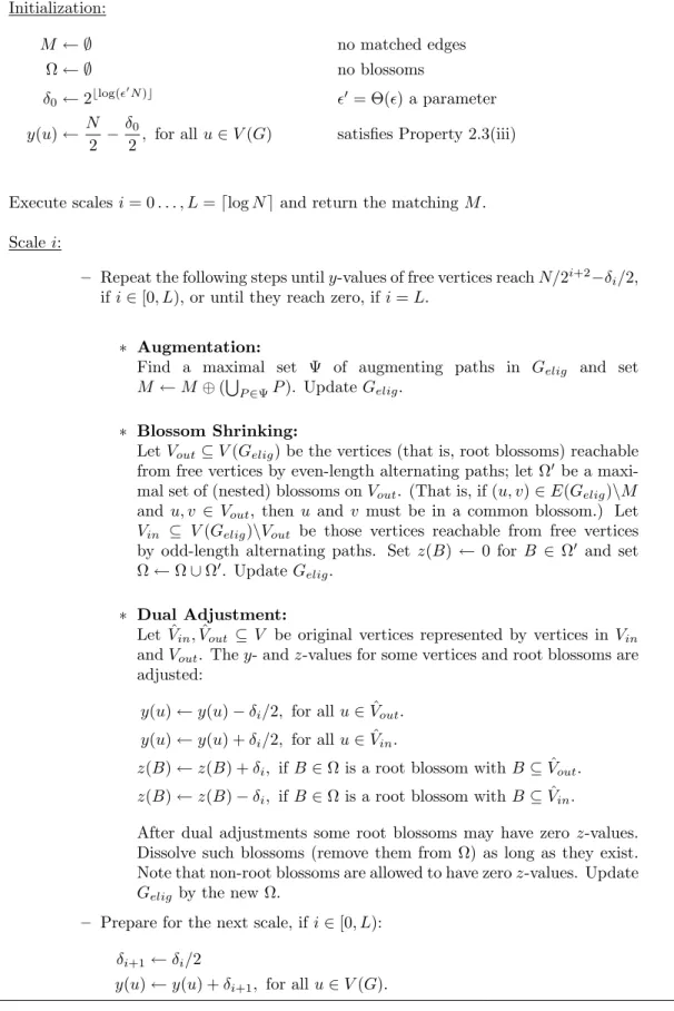
Initialization: M ← ∅ no matched edges Ω← ∅ no blossoms δ0←2blog( 0N)c 0= Θ() a parameter y(u)← N 2 − δ0
2, for allu∈V(G) satisfies Property 2.3(iii)
Execute scalesi= 0. . . , L=dlogNeand return the matchingM.
Scalei:
– Repeat the following steps untily-values of free vertices reachN/2i+2−δ i/2,
ifi∈[0, L), or until they reach zero, ifi=L.
∗ Augmentation:
Find a maximal set Ψ of augmenting paths in Gelig and set
M ←M ⊕(S
P∈ΨP). UpdateGelig.
∗ Blossom Shrinking:
LetVout ⊆V(Gelig) be the vertices (that is, root blossoms) reachable
from free vertices by even-length alternating paths; let Ω0 be a maxi-mal set of (nested) blossoms onVout. (That is, if (u, v)∈E(Gelig)\M
and u, v ∈ Vout, thenu and v must be in a common blossom.) Let
Vin ⊆ V(Gelig)\Vout be those vertices reachable from free vertices
by odd-length alternating paths. Set z(B) ← 0 for B ∈ Ω0 and set Ω←Ω∪Ω0. UpdateG
elig.
∗ Dual Adjustment:
Let ˆVin,Vˆout ⊆ V be original vertices represented by vertices in Vin
andVout. They- andz-values for some vertices and root blossoms are
adjusted:
y(u)←y(u)−δi/2, for allu∈Vˆout.
y(u)←y(u) +δi/2, for allu∈Vˆin.
z(B)←z(B) +δi, ifB∈Ω is a root blossom withB ⊆Vˆout.
z(B)←z(B)−δi, ifB∈Ω is a root blossom withB ⊆Vˆin.
After dual adjustments some root blossoms may have zero z-values.
Dissolve such blossoms (remove them from Ω) as long as they exist. Note that non-root blossoms are allowed to have zeroz-values. Update Geligby the new Ω.
– Prepare for the next scale, ifi∈[0, L): δi+1←δi/2
y(u)←y(u) +δi+1, for allu∈V(G).
2.4.2 Analysis and Correctness
Lemma 2.6. After the Augmentation and Blossom Shrinking stepsGelig contains no augmenting path, nor is there a path from a free vertex to a blossom.
Proof. Suppose there is an augmenting pathP inGelig after augmenting along paths
in Ψ. Since Ψ is maximal, P must intersect some P0 ∈ Ψ at a vertex v. However, after the Augmentation step every edge inP0 will become ineligible, so the matching edge (v, v0)∈M is no longer inG
elig, contradicting the fact that P consists of eligible edges. Since Ω0 is maximal there can be no blossom reachable from a free vertex in Gelig after the Blossom Shrinking step.
Lemma 2.7. (Parity of y-values) Let R ⊆ V(Gelig) be the set of vertices reachable
from free vertices by eligible alternating paths, at any point in scale i. Let Rˆ⊆V(G)
be the set of original vertices represented by those in R. Then the y-values of Rˆ
-vertices have the same parity, as a multiple of δi/2.
Proof. Assume, inductively, that before the Blossom Shrinking step, all vertices in
a common blossom have the same parity, as a multiple of δi/2. Consider an eligible path P = (B0, B1, . . . , Bk) in Gelig, where the {Bj} are either vertices or blossoms in Ω and B0 is unmatched in Gelig. Let (u0, v1),(u1, v2), . . . ,(uk−1, vk) be the
G-edges corresponding to P, where uj, vj ∈Bj. By the inductive hypothesis, uj and vj have the same parity, and whether (uj, vj+1) is matched or unmatched, Definition 2.5
implies that yz(uj, vj+1)/δi is an integer, which implies y(uj) and y(vj+1) have the
same parity as a multiple of δi/2. Thus, the y-values of all vertices in B0∪ · · · ∪Bk
have the same parity as a free vertex in B0, whose y-value is equal to every other
free vertex, by Property 2.3(v). Since new blossoms are formed by eligible edges, the inductive hypothesis is maintained after the Blossom Shrinking step. It is also maintained after the Dual Adjustment step since they-values of vertices in a common
Lemma 2.8. The algorithm preserves Property 2.3.
Proof. Property 2.3(v) (free vertex duals) is obviously maintained since only free
ver-tices have their y-values decremented in each Dual Adjustment step. Property 2.3(ii) (active blossoms) is also maintained since all the new root blossoms found in the Blossom Shrinking step are contained in Vout and will have positivez-values after ad-justment. Furthermore, each root blossom whose z-value drops to zero is dissolved, after Dual Adjustment. At the beginning of scale i all y- and z-values are integer multiples of δi/2 and δi, respectively, satisfying Property 2.3(i) (granularity). This property is clearly maintained in each Dual Adjustment step.
It remains to show that the algorithm maintains Property 2.3(iii),(iv) (near dom-ination, near tightness). Let e= (u, v) be an arbitrary edge and ibe the scale. First consider the dual adjustments made at the end of the scale; let yz and yz0 be the function before and after adjustment. At the end of scaleiwe haveyz(e)≥wi(e)−δi. Eachy-value is incremented byδi+1 andwi+1(e)≤wi(e)+δi+1, henceyz0(e) =yz(e)+
2δi+1 ≥wi(e)≥wi+1(e)−δi+1, which preserves Property 2.3(iii). Ife∈M∪SB∈ΩEB is a typej edge, then at the end of the scaleyz(e)≤wi(e) + 2(δj−δi). By the same reasoning as above,yz0(e) = yz(e) + 2δi
+1≤wi(e) + 2δj−δi ≤wi+1(e) + 2(δj−δi+1),
preserving Property 2.3(iv).
If e is placed in M during an Augmentation step or it is a non-M edge placed in
S
B∈ΩEB during a Blossom Shrinking step then e has type i and yz(e) =wi(e)−δi,
which satisfies Property 2.3(iv). Now consider a Dual Adjustment step. If neither u nor v is in ˆVin∪Voutˆ or if u, v are in the same root blossom B ∈ Ω, then yz(e) is unchanged, preserving Property 2.3. The remaining cases depend on whether (u, v) is inM or not, whether (u, v) is eligible or not, and whether bothu, v ∈Vinˆ ∪Voutˆ or not.
Case 1: e6∈M, u, v ∈Vˆin∪Vˆout Ife is ineligible thenyz(e)> wi(e)−δi. However, by Lemma 2.7 (parity ofy-values) we know (yz(e)−wi(e))/δi is an integer, soyz(e)≥ wi(e) before adjustment andyz(e)≥wi(e)−δi after adjustment (if bothu, v ∈Vout),ˆ which preserves Property 2.3(iii). If e is eligible then at least one of u, v is in ˆVin, otherwise another blossom or augmenting path would have been formed, so yz(e) cannot be reduced, which also preserves Property 2.3(iii).
Case 2: e ∈ M, u, v ∈ Vinˆ ∪Voutˆ Since u, v ∈ Vinˆ ∪Vout, Lemma 2.7 (parity ofˆ y-values) guarantees that (yz(e)−wi(e))/δi is an integer. The only way e can be ineligible is if yz(e) = wi(e)−δi and u, v ∈ Vˆin, hence yz(e) = wi(e) after dual adjustment, which preserves Property 2.3(iii),(iv). On the other hand, if e is eligible thenu∈Vinˆ andv ∈Vout. It cannot be thatˆ u, v ∈Vout, otherwiseˆ e would have been included in an augmenting path or root blossom. In this case yz(e) is unchanged, preserving Property 2.3(iii),(iv).
Case 3: e 6∈M, v 6∈Vinˆ ∪Voutˆ If e is eligible then u ∈Vinˆ and yz(e) will increase. If it is ineligible then yz(e)≥wi(e)−δi/2 before adjustment and yz(e)≥ wi(e)−δi after adjustment. In both cases Property 2.3(iii) is preserved.
Case 4: e ∈ M, v 6∈ Vinˆ ∪ Voutˆ It must be that e is ineligible, so u ∈ Vinˆ and yz(e)−wi(e) is either negative or an odd multiple of δi/2. If e is type j then, by Property 2.3(i),(iv) (granularity and near tightness), yz(e) ≤ wi(e) + 2(δj −δi)−
δi/2 before adjustment and yz(e) ≤ wi(e) + 2(δj −δi) after adjustment, preserving Property 2.3(iv).
Lemma 2.9. Let i≤L be the scale index. Then
(i) For i < L, all edges eligible at any time in scales 0 through i have weight at
(ii) For any i, if e∈M then yz(e)≤(1 + 40)w(e).
Proof. Part 1 The last search for augmenting paths in scale i begins when the
y-values of free vertices are N/2i+2, and strictly less than y-values of other vertices, by
Property 2.3(v). An unmatched edge e = (u, v) can only be eligible at this scale if yz(e) = wi(e)−δi ≤w(e)−δi. Hence w(e)≥y(u) +y(v) +δi ≥N/2i+1+δi.
Part 2 Let e be a type j edge in M during scale i. Property 2.3(iv) states that yz(e)−wi(e) ≤ 2(δj −δi). Since wi(e) ≤ w(e) it also follows that yz(e)−w(e) ≤
2δj−2δi <2blog(0N)c−j+1
≤0N/2j−1. By part 1, a type j edge must have weight at
least N/2j+1+δj, so yz(e)−w(e)<40 ·w(e).
Lemma 2.10. After scale L=dlogNe, M is a (1−50)-MWM.
Proof. The final scale ends with free vertices having zero y-values. Property 2.3(iii)
holds w.r.t. δL = δ0/2L ≤ 0N/2L ≤ 0 and Lemma 2.9 states that yz(e) ≤ (1 +
40)w(e). By Lemma 2.4 w(M)≥(1−50)w(M∗).
Theorem 2.11. A (1−)-MWM can be computed in time O(m−1logN).
Proof. Each Augmentation and Blossom Shrinking step takes O(m) time [35, §8]
using a modified depth-first search. (Finding a maximal set of augmenting paths is significantly simpler than finding a maximal set of minimum-length augmenting paths, as is done in [47, 66].) Each Dual Adjustment step clearly takes linear time. Scale i < L = dlogNe begins with free vertices’ y-values at N/2i+1 −δi and ends
with them at N/2i+2 − δi. Since y-values are decremented by δi/2 in each Dual
Adjustment step there are exactly (N/2i+2)/(δi/2) =N/(2δ
0)< 0−1 such steps. The
last inequality follows since δ0 = 2blog(
0N)c
> 0N/2. The final scale begins with free vertices’ y-values at N/2L+1 − δ
L and ends with them at zero, so there are fewer than (N/2L+1)/(δ
L/2) = (N/2L+1)/2blog(
0N)c−(L+1)
= 2logN−blog(0N)c
< 20−1 Dual
Adjustment steps. Lemma 2.10 guarantees that the final matching is a (1−)-MWM for 0 =/5. Thus, the total running time is O(m−1logN).
2.4.3 A Linear Time Algorithm
Our O(m−1logN)-time algorithm requires few modifications to run in linear
time, independent ofN. In fact, the algorithm as it appears in Figure 2.2 requires no modifications at all: we only need to change the definition of eligibility and, in each scale, avoid scanning edges that cannot be eligible or part of augmenting paths or blossoms. From Lemma 2.9(i) it is helpful to index edges according to the first scale in which they may be eligible.
Definition 2.12. Define µi = N/2i+1 +δi, for i < L, and µL = 0. For any edge e,
define scale(e) =i such that w(e)∈[µi, µi−1).
Definition 2.13 redefines eligibility. The differences with Definition 2.5 are under-lined.
Definition 2.13. At scale i, an edgee iseligibleif at least one of the following hold: (i) e∈EB for some B ∈Ω.
(ii) e6∈M and yz(e) =wi(e)−δi.
(iii) e∈M, wi(e)−yz(e) is a nonnegative integer multiple of δi, and scale(e)≥i−γ, whereγ def= dlog0−1e.
Let Eelig be the set of eligible edges and let Gelig = (V, Eelig)/Ω be the unweighted graph obtained by deleting ineligible edges and contracting root blossoms.
Lemma 2.14. Using Definition 2.13 of eligibility rather than Definition 2.5, Prop-erty 2.3(i),(ii),(iii),(v) is maintained and PropProp-erty 2.3(iv) (near tightness) holds in
the following weaker form. Let e ∈M ∪S
B∈ΩEB be a type j edge with scale(e) =i.
Then yz(e)≤wk(e) + 2(δj −δk) at any scale k ∈[i, i+γ] and yz(e)≤wk(e) + (3 + 30/2)δi <(1 + 70)w(e) for k > i+γ.
Proof. In scalesithroughi+γ Property 2.3(iv) is maintained as the two definitions of eligibility are the same. At the beginning of scalei+γ+1,eis no longer eligible and the y-values of free vertices areN/2i+γ+2−δi
+γ+1/2. From this moment on, they-values of
free vertices are incremented by a total ofP
l≥i+γ+2δl(the dual adjustments following
scales i+γ+ 1 through logN−1) and decremented a total ofN/2i+γ+2−δi
+γ+1/2 +
P
l≥i+γ+2δl (in the Dual Adjustment steps following searches for augmenting paths
and blossoms). Each adjustment to a free y-value by some quantity ∆ may cause yz(e) to increase by 2∆. This clearly occurs in the dual adjustments following each scale asy(u) and y(v) are incremented by ∆. Following a search for blossoms it may be that u, v ∈ Vin, which would also causeˆ y(u) and y(v) to each be incremented by ∆. Note that y(u), y(v) cannot be decremented in scales i+γ+ 1 forward; if either were in ˆVout after a search for blossoms then e would have been eligible, which is a contradiction. Thus Property 2.3(iii) (near domination) is maintained fore. Putting this all together, it follows that from scale k≥i+γ+ 1 forward,
yz(e)≤wk(e) + 2(δj−δk) + 2· N/2i+γ+2−δi+γ+1/2 + 2·
X
l≥i+γ+2
δl
!
< wk(e) + 2δi+ 2 0N/2i+2+ 32δi+γ+1
j ≥i, defn. of γ < wk(e) + 2δi+ 2 δi+1+3
0 2 δi+1 0N/2i+2 < δi +1, defn. of γ. =wk(e) + (3 + 30/2)δi ≤wk(e) + (3 + 30/2)(0N/2i) δi ≤0N/2i <(1 + 70)w(e) w(e)≥wk(e)> N/2i+1, 0 <1/3
Lemma 2.15. Let e1 = (u, v) be an edge with scale(e1) = i and let e0 = (u0, u) and
e2 = (v, v0) be the M-edges incident to u and v at some time after scale i. Then at least one of e0 and e2 exists, and its scale is at most i+ 2.
Proof. Following the last Dual Adjustment step in scale i the y-values of free ver-tices are N/2i+2 − δ
i/2. It cannot be that both u and v are free at this time, otherwise yz(e1) = y(u) + y(v) = N/2i+1 −δi = µi −2δi < wi(e1)− δi,
violat-ing Property 2.3(iii) (near domination). Thus, either u or v is matched for the remainder of the computation. If e1 is matched the claim is trivial, so, assuming
the claim is false, whenever e0, e2 exist we have scale(e0),scale(e2)≥ i+ 3. That is,
w(e0), w(e2)< µi+2 =N/2i+3+δi+2.
e1 cannot be in a blossom without e0 ore2 also being in the blossom. Let Bl⊂Ω be the blossoms containing el at a given time. The laminarity of blossoms ensures that either B1 ⊆ B0 or B1 ⊆ B2. Suppose it is the former, that is, e0 exists and e2
may or may not exist. Then, if the current scale is k ≥ i+ 3, by Property 2.3(iii) (near domination)yz(e1) =y(u) +y(v) +PB∈B1z(B)≥wk(e1)−δk. By Lemma 2.14
(near tightness) y(u) +P
B∈B1 < yz(e0) ≤wk(e0) + (3 + 3
0/2)δi
+3 and, if e2 exists,
y(v)< yz(e2)≤wk(e2) + (3 + 30/2)δi+3. These inequalities follow from the definition
of yz, the containmentB1 ⊆ B0 and the fact thate0 and e2 can only be at scalei+ 3
or higher. Without loss of generality we can assume y(u) +P
B∈B1 ≥y(v); note that
if e2 does not exist then y(v) < y(u) +PB∈B1, by Property 2.3(v). Putting these
inequalities together we have
wk(e1)≤y(u) +y(v) +
X B∈B1 z(B) +δk near domination ≤2 y(u) + X B∈B1 z(B) ! +δk
<2(wk(e0) + (3 + 30/2)δi+3) +δk near tightness
and therefore
w(e0)≥ 12(wk(e1)−δi) 8δi+3 =δi
≥N/2i+2 scale(e1) = i, wk(e1)≥µi =N/2i+1+δi
> N/2i+3+δi+2 =µi+2
This contradicts the fact that scale(e0)≥ i+ 3, since such edges have w(e0)< µi+2
by definition.
Theorem 2.16. A (1−)-MWM can be computed in time O(m−1log−1).
Proof. We execute the algorithm from Figure 2.2 where Gelig refers to the eligible
subgraph as defined in Definition 2.13. We need to prove several claims: (i) the algorithm does return a (1−)-MWM for suitably chosen 0 = Θ(), (ii) the number of scales in which an edge could possibly participate in an augmenting path or blossom is log−1+O(1), and (iii) it is possible in linear time to compute the scales in which
each edge must participate. Part (i) follows from Lemmas 2.4 and 2.14. Sinceyz(e)≤
(1 + 70)w(e) for any e ∈ M (by Lemma 2.14) and δL ≤ 0, Lemma 2.4 implies that M is a (1−)-MWM when0 =/8.
Turning to part (ii), consider an edge e with scale(e) =i. By Lemma 2.9(i) e can be ignored in scales 0 through i−1. If e= (u, v)∈M, according to Definition 2.13, e will be ineligible in scalesi+γ+ 1 through logN. After scale i+γ no augmenting path or blossom can contain e, so we can put it in the final matching and remove from consideration all edges incident to u or v. Now suppose thate 6∈M at the end of scale i+γ + 2. Lemma 2.15 states that either u or v is incident to a matched edge e0 with scale(e0)≤i+ 2, which by the argument above, will be put in the final
matching. Therefore we can remove e from further consideration. Thus, to execute the algorithm we only need to consider e in scales scale(e) through scale(e) +γ + 2, that is, γ+ 3 =dlog0−1e+ 3≤log−1+ 7 scales in total.
We have narrowed our problem to that of computing scale(e) for all e. This is equivalent to computing the most significant bit (MSB(x) = blog2xc) in the binary representation ofw(e). Once the MSB is known, scale(e) can be just one of two possi-ble values. MSBs can be computed in a number of ways using standard instructions. It is trivial to extract MSB(x) after converting x to floating point representation. Fredman and Willard [31] gave an O(1) time algorithm using unit time multiplica-tion. However, we do not need to rely on floating point conversion or multiplicamultiplica-tion. In Section 2.2 we showed that without loss of generality logN ≤2 logn. Using a neg-ligibleO(nβ) space and preprocessing time we can tabulate the answers onβ·logn-bit integers, where β≤1, then compute MSBs with 2β−1 =O(1) table lookups.
2.4.4 Conclusion
We have given the first linear time (1−)-approximate MWM algorithm for ar-bitrarily small . Our result is a major improvement over the previous best linear time algorithm, which guaranteed only (2/3 − )-approximations. [67, 51]. How-ever, making our algorithm suitable for parallel computing is a major challenge. The best efficient parallel/distributed approximate MWM algorithm guarantees only 1/2-approximations. [44]. Improving the exact MWM algorithms is also a challenge for us.
CHAPTER III
Connectivity Oracle for Failure-Prone Graphs
The main result in this chapter is a new, space efficient data structure that can quickly answer connectivity queries after recovering from d vertex failures.1 The
recovery time is polynomial in d and logn but otherwise independent of the size of the graph. After processing the failed vertices, connectivity queries are answered in O(d) time. The space used by the data structure is roughlymn, for any fixed >0, whereonly affects the polynomial in the recovery time. The exact tradeoffs are given in Theorem 3.1. Our data structure is the first of its type. To achieve comparable query times using existing data structures we would need either Ω(nd) space [19] or Ω(dn) recovery time [49].
It is easy to see that handling dvertex failures can be much harder than handling only d edge failures, since a vertex failure can cause the failure of as many as n−1 edges, which may have a large impact on the graph connectivity. First, we reduce the problem of d-edge failure recovery on a spanning forest of G to 2D range searching, that is, searching for edges reconnecting the split trees is equivalent to searching ele-ments in rectangles in a 2D table. The time is quadratic of the number of deleted tree edges. Then we perform a “sparsification” on the spanning forest ofGwhich restricts the degree bound of failed vertices in a set of forests when given any set of d failed 1This result appears in Duan and Pettie’s paper “Connectivity Oracles for Failure Prone
vertices. In the complexities, there is a positive parameter c controlling the tradeoff between the space and the recovery time from vertex failures. Whencbecomes larger, the space becomes smaller but the recovery time gets larger. Theorem 3.1 gives a precise statement of the capabilities and time-space tradeoffs of our structure:
Theorem 3.1. Let G= (V, E) be a graph with m edges and n vertices and let c≥1
be an integer. A data structure with size S =O(d1−2/cmn1/c−1/(clog(2d))log2n) can be
constructed in O(S)˜ time that supports the following operations. Given a set D of
at most d failed vertices, D can be processed in O(d2c+4log2nlog logn) time so that
connectivity queries w.r.t. the graph induced by V\D can be answered in O(d) time.
Overview. In Section 3.1 we present the Euler Tour Structure, which plays a key role in our vertex-failure oracle and can be used independently as an edge-failure oracle. In Sections 3.2 and 3.3 we define and analyze the redundant graph represen-tation (called the high degree hierarchy) mentioned earlier. In Section 3.4 we provide algorithms to recover from vertex failures and answer connectivity queries.
3.1
The Euler Tour Structure
In this section we describe the ET-structure for handling connectivity queries avoiding multiple vertex and edge failures. When handling only d edge failures, the performance of the ET-structure is incomparable to that of Pˇatra¸scu and Thorup [49] in nearly every respect.2 The strength of the ET-structure is that if the graph can be
covered by a low-degree tree T, the time to delete a vertexis a function of its degree 2The ET-structure is significantly faster in terms of construction time (near-linear vs. a large
polynomial or exponential time) though it uses slightly more space: O(mlogn) vs. O(m). It
handles d edge deletions exponentially faster for bounded d (O(log logn) vs. Ω(log2nlog logn))
but is slower as a function of d: O(d2log logn) vs. O(dlog2nlog logn) time. The query time is
the same for both structures, namely O(log logn). Whereas the ET-structure naturally maintains
a certificate of connectivity (a spanning tree), the Pˇatra¸scu-Thorup structure requires modification and an additional logarithmic factor in the update time to maintain a spanning tree.
in T; incident edges not in T are deleted implicitly. We prove Theorem 3.2 in the remainder of this section.
Theorem 3.2. Let G= (V, E) be a graph, with m = |E| and n =|V|, and let F =
{T1, . . . , Tt} be a set of vertex disjoint trees in G. (The Ti’s do not necessarily span
a connected component of G.) There is a data structure ET(G,F) occupying space
O(mlogn)(for any fixed >0) that supports the following operations. SupposeDis
a set of failed edges, of which dare tree edges in F andd0 are non-tree edges. Deleting
D splits some subset of the trees in F into at most 2d trees F0 = {T0
1, . . . , T20d}. In O(d2log logn +d0) time we can report which pairs of trees in F0 are connected by
an edge in E\D. In O(min{log logn,logd}) time we can determine which tree in F0
contains a given vertex.
Our data structure uses as a subroutine Alstrup et al.’s data structure [2] for range reporting on the integer grid [U]×[U]. They showed that given a set of N points, there is a data structure with size O(NlogN), where >0 is fixed, such that given x, y, w, z ∈[U], the set of points in [x, y]×[w, z] can be reported in O(log logU +k) time, where k is the number of reported points. Moreover, the structure can be built inO(NlogN) time.
For a tree T, let L(T) be a list of its vertices encountered during an Euler tour of T (an undirected edge is treated as two directed edges), where we only keep the
first occurrence of each vertex. One may easily verify that removing f edges from
T partitions it into f + 1 connected subtrees and splits L(T) into at most 2f + 1 intervals, where the vertices of a connected subtree are the union of some subset of the intervals. To build ET(G = (V, E),F) we build the following structure for each pair of trees (T1, T2) ∈ F × F; note that T1 and T2 may be the same. Let m0
be the number of edges connecting T1 and T2. Let L(T1) = (u1, . . . , u|T1|), L(T2) =
(v1, . . . , v|T2|), and let U = max{|T1|,|T2|}. We define the point set P ⊆ [U]×[U]
d1 edges in T1, d2 in T2, and d0 non-tree edges. Removing D splits T1 and T2 into
d1+d2+ 2 connected subtrees and partitionsL(T1) into a setI1 ={[xi, yi]}i of 2d1+ 1
intervals and L(T2) into a set I2 = {[wi, zi]}i of 2d2+ 1 intervals. For each pair i, j
we query the 2D range reporting data structure for points in [xi, yi]×[wj, zj]∩P. However, we stop the query the moment it reports some point corresponding to a non-failed edge, i.e., one in E\D. Since there are (2d1 + 1)×(2d2 + 1) queries and
each failed edge in Dcan only be reported in one such query, the total query time is O(d1d2log logU+|D|) =O(d1d2log logn+d0). See Figure 3.1 for an illustration.
The space for the data structure (restricted to T1 and T2) is O(|T1|+ |T2| +
m0logn). We can assume without loss of generality3 that |T
1|+|T2| < 4m0, so the
space for the ET-structure onT1 andT2 isO(m0logn). Since each non-tree edge only
appears in one such structure the overall space forET(G,F) is O(mlogn). For the last claim of the Theorem, observe that if a vertexulies in an original treeT1 ∈ F, we
can determine which tree inF0contains it by performing a predecessor search over the left endpoints of intervals inI1. This can be accomplished inO(min{log logn,logd1})
query time using a van Emde Boas tree [62] or sorted list, whichever is faster. Corollary 3.3 demonstrates how ET(G,·) can be used to answer connectivity queries avoiding edge and vertex failures.
Corollary 3.3. The data structure ET(G= (V, E),{T}), where T is a spanning tree
of G, supports the following operations. Given a setD⊂E of edge failures, Dcan be
processed in O(|D|2log logn) time so that connectivity queries in the graph (V, E\D)
3The idea is to remove irrelevant vertices and contract long paths of degree-2 vertices. More
formally: letV1⊆V(T1) be those vertices incident to one of them0 non-tree edges. We can replace T1 by an equivalent tree ˜T1 with less than 2m0 vertices via the following steps: (1) Let T10 be the
minimal subtree of T1 in which V1 remains connected, then (2) Let ˜V1 be the union of V1 and
all branching vertices, i.e., those with degree at least 3, in T0
1 (note |V˜1| < 2|V1|), then (3) Let
˜
T1 = ( ˜V1,E˜1), where (u, v)∈E˜1 if there is a path (u, . . . , v) inT10, none of whose interior vertices
are in ˜V1. The removal of an edge from T1 can clearly be simulated by removing an edge from ˜T1.
To determinewhichedge in ˜T1 we only need to perform a predecessor search over ˜V1. Using a van
Emde Boas tree, such queries can be answered inO(log log|T1|) =O(log logn) time. We only need
u1 u2 u3 u4 u5 u6 u7 u8 u9 u10 u11 u12 v1 v2 v3 v4 v5 v6 v7 v8 v9 T1 T2 (A) 1 3 5 7 9 11 1 3 5 7 9 T2: T