Regional Input-Output Analysis

(1)

Web Book of Regional Science

Regional Research Institute

2020

Geoffrey J. D. Hewings

Follow this and additional works at: https://researchrepository.wvu.edu/rri-web-book

Recommended Citation

Hewings, Geoffrey J. D., "Regional Input-Output Analysis" (2020). Web Book of Regional Science. 10. https://researchrepository.wvu.edu/rri-web-book/10

This Book is brought to you for free and open access by the Regional Research Institute at The Research Repository @ WVU. It has been accepted for inclusion in Web Book of Regional Science by an authorized administrator of The Research Repository @ WVU. For more information, please contact

(2)

The Web Book of Regional Science

The Web Book of Regional Science is offered as a service to the regional research community in

an effort to make a wide range of reference and instructional materials freely available

online. Roughly three dozen books and monographs have been published as Web Books of

Regional Science. These texts covering diverse subjects such as regional networks, land use,

migration, and regional specialization, include descriptions of many of the basic concepts,

analytical tools, and policy issues important to regional science. The Web Book was launched in

1999 by Scott Loveridge, who was then the director of the Regional Research Institute at West

Virginia University. The director of the Institute, currently Randall Jackson, serves as the Series

editor.

When citing this book, please include the following:

Hewings, Geoffrey J.D.

“

Regional Input-Output Analysis

”

. Web Book of Regional Science.

Regional Research Institute, West Virginia University. Edited by

Grant Ian Thrall, 1985; Randall

Jackson, 2020.

(5)

(6)

Contents

ACKNOWLEDGEMENTS 5

SERIES EDITOR’S INTRODUCTION 7

1 INTRODUCTION 8

2 LINKS BETWEEN ECONOMIC BASE, KEYNESIAN,

AND INPUT-OUTPUT MODELS 10

2.1 Standard Macro-Level Accounting Framework . . . 10

2.2 The Economic Base Model. . . 11

2.3 The Link with the Input-Output Model . . . 13

2.4 The Regional Input-Output Accounting Framework: Initial Steps . . . 14

3 THE BASIC REGIONAL INPUT-OUTPUT MODEL 17 3.1 Elements of the Input-Output Table . . . 17

3.2 Links with National Accounts . . . 19

3.3 Regional Input-Output Model. . . 20

3.4 Income and Employment Multipliers . . . 23

3.5 Summary . . . 26

4 APPLICATIONS 27 4.1 Impact Analysis with an Input-Output Model . . . 27

4.2 Using an Input-Output Model in Project Appraisal . . . 29

4.3 Summary . . . 32

5 CONSTRUCTION OF REGIONAL INPUT-OUTPUT MODELS 33 5.1 Nonsurvey Techniques . . . 33

5.2 Partial Survey Techniques . . . 35

5.3 Most Important Coefficient Estimation . . . 36

6 MULTIREGIONAL AND INTERREGIONAL INPUT-OUTPUT MODELS 41 6.1 Interregional Input-Output Framework . . . 41

6.2 The Multiregional Input-Output Model . . . 43

6.3 The Interregional Model in an Entropy Formulation . . . 44

6.4 Summary . . . 46

7 EXTENSIONS TO INPUT-OUTPUT ANALYSIS 47 7.1 Miyazawa’s Framework. . . 47

7.2 The General Social Accounting Framework . . . 51

7.3 The Batey-Madden Activity Analysis Framework . . . 53

7.4 Links with the Labor Market . . . 54

7.5 Linear Programming Input-Output Links . . . 56

7.6 Further Extensions . . . 58

7.7 Summary . . . 58

8 FUTURE DIRECTIONS AND RESEARCH NEEDS 59 8.1 Relaxing the Assumptions . . . 59

8.2 Dynamic Modeling . . . 59

8.3 New Accounting Systems . . . 59

8.4 Use in Policy Analysis . . . 60

8.5 Conclusions . . . 60

(7)

(8)

(9)

ACKNOWLEDGMENTS

The comments and suggestions provided by Gordon Mulligan, Adrian Esparza, Grant Thrall, Randall Jackson, Breadan O’hUallachain, and the reviewer, Adam Rose, are gratefully appreciated. My introduction to regional input-output analysis was provided by Charles Tiebout almost twenty years ago. William Miernyk’sElements of Input-Output Analysis served as an excellent reference for the novitiate input-output analyst. Modern regional analysis owes a great deal to their important contributions; I hope the spirit of their influence is contained within this small volume.

(10)

(11)

SERIES EDITOR’S INTRODUCTION

Input-output analysisis a method by which the flow of production can be traced among the various sectors of the economy, through to final demand or export. The most fundamental problem of input-output analysis is to calculate the necessary output levels of each industry required to achieve a final output. Included among the uses of input-output analysis is the ability to determine the following: What is the effect upon the local ecoomy from the introduction of a new firm? What are the economic linkages between regions and how is equilibrium between regions achieved? What if the supply of an input in one region becomes restricted through some bottleneck?

The foundation of modern input-output analysis can be traced to work in both economics and geography. The linkages to geography have been largely through the earlier analysis of urban economic base and city classification. In economics the work can be traced to the 1930s pioneeering efforts of W. W. Leontief, which led to his receiving the Nobel Prize. Much of the recent contributions in input-output analysis falls within the purview of regional science, the overlap of interests in economics, geography, city and regional planning, and engineering. This literature has refined the ability of input-output analysts to work with incomplete data sets, arrive at stable and accurate estimates, and apply the general input-output method in practice to actual planning situations. With the exception of gravity and spatial interaction models, no topic in scientific geography has achieved greater practical application.

Professor Geoffrey Hewings is recognized as one of the leading contemporary scholars in input-output modeling, and has presented here one of the most readable introductions to the input-output problem and the contemporary literature that refines the technique. At the same time, save for the requirement that the reader have a grasp of elementary matrix algebra, Hewings keeps the book entirely at a level that can be understood by a reader who is encountering the material for the first time.

Professor Hewings first establishes the historical links between input-output models and the earlier macroe-conomic accounting framework, emacroe-conomic base models, and the fundamental regional input-output model. Following the development of the basic model, and a discussion of the interpretation of the components of the model such as income and employment multipliers, Hewings discusses how the general model can be applied in practice. On applying the model, he first describes how to construct the input-output tables for interregional and multiregional input-output matrices; he then presents a general discussion of estimation; and finally he presents practical examples of implementing the input-output model. The book brings the reader up to a discussion of the contemporary research frontier and likely future developments in input-output analysis.

This book will prove to be a valuable resource to students and practitioners of the planning sciences, including urban and regional economics, regional science, engineering, public administration, business management science, city and regional planning, as well as scientists in economic geography.

-Grant Ian Thrall

(12)

1

INTRODUCTION

Imagine a national economythat has been divided into a set of regions. Within each region, grouped into sectors, there is a set of firms producing a variety of commodities that are consumed by other firms in the course of the production of other more finished commodities (e.g., automobile parts are assembled into a finished automobile), consumers, government, export markets, or other firms using these commodities as investment goods. In addition to engaging in sales activities, firms are also active in the purchase of commodities and other inputs-labor, entrepreneurial skills, as well as commodities purchased from outside the region. It would not be unusual to find in a region of several million people well over 100,000 firms producing as many as half a million or more commodities.

Suppose that a newly elected national-level or federal government proposes to reorient priorities away from social spending to defense spending. What will be the resulting impact on our regional economy and other regions making up this nation? As a result of these changes or in response to other stimuli, assume a new firm locates in the region employing 2000 people. What will be the impact of this new activity on the region? From another perspective, assume that the comparative advantage that the region once enjoyed in the export of its commodities is eroded, with the resulting closure of many local firms and an increase in regional unemployment levels. Again, what will be the impact of this activity change on the regional economy? With the large number of firms, commodities, consumers, and other actors in the regional economy, it should be obvious that tracing the impacts on a firm-by-firm or consumer-by-consumer basis would be a daunting proposition. Clearly, we need some accounting system into which these interactions can be placed in the hope that some analytical method could be employed to trace the impacts in a systematic fashion. In a sense, we are going to have to sacrifice the richness of the reality of the regional economy for some reduced-form picture or model that is tractable and, we hope, representative as far as is possible of the micro-level interactions. As happens with a great deal of analytical work in the social sciences, the gains from model development are not without cost; as we shall see, this is the case in the development of a family of analytical tools that are referred to associal accounting systems. Regional input-output analysis is one subset of these accounting systems.

This book will focus on some of the more elementary versions of these social accounting models (or SAMs) to provide a guide to their underlying theoretical structure and to explore ways in which they can be used to answer the sort of questions posed in the preceding paragraph. Thereafter, some excursions will be made into new developments that have extended the range and analytical complexity of these models, thereby enabling us to use them to answer more complex questions. One of the most interesting features of SAMs is that, on the one hand, they are strongly linked with standard macroeconomic accounting principles, and, on the other hand, they can be linked with many of the more traditional avenues of inquiry in the geographic and regional science fields. For example, interest in spatial interaction of commodities or individuals can be linked with a SAM framework; hence, we have the capability to explore the effects of the federal program changes alluded to earlier, not only on the structure of the economic system but potentially on the degree to which these changes will in turn promote changes in regional attractiveness for migration decisions.

These changes, in their turn, will have a further impact on the structure of production in the regional economy. How? Consider the case of a new firm opening up in the region. Because we are assuming a freely mobile society, with no restrictions on interregional movement, competition for the new jobs may come not only from local residents but from other persons in-migrating from other regions. Assuming that total employment rises and that some of this increase is associated with in-migration, it is likely that the demand for local services will rise. The new in-migrants and their families will demand commodities, public services such as schools, health care and so forth, and thus create the necessary conditions for an expansion of the economic base of the region. Whether this occurs will depend in part on the degree of excess capacity that may already exist in some firms and public services.

Without getting too embroiled in the details at this stage, we can begin to see a very strong link emerging between the structure of production and the structure of consumption. Changes in either component of the regional economy are likely to lead to changes in the other and, in turn, to further changes in the first component. Viewing the regional economic system in this fashion--as a broadly-based system of interdependence--provides substantial insights into the functioning of regional economies. It will enable us to

(13)

begin to understand why regional economies may or may not be responsive to changes that may take place at the national or even at the international level, why some regional economies are exhibiting characteristics of decline, why others are growing, and why still others seem to be relatively immune from the effects of major structural changes that have been observed in many Western economies over the last two decades. The modeling systems to be described here will not provide answers to all our questions; many of these models contain very restrictive assumptions, precluding their use in many contexts. Neither are these models to be considered theories of regional economic growth and development. For the most part, they are empirical models that, although resting on some theoretical assumptions, are not exclusively associated with any one paradigm. In fact, these models have one very interesting attribute - they have been used in centrally planned, socialist, free market, developed, and developing economies alike. This flexibility provides one of their attractions.

The field of regional social accounting in general and input-output analysis in particular has a rich legacy. Some of the more prominent economists of this century have worked in this area; four - Tinbergen in 1969, Kuznets in 1971, Leontief in 1973, and Stone in 1984 - have been awarded the Nobel Prize in Economics for their work in developing many of the accounting frameworks that will be used in this book. At the regional and interregional level, input-output analysis has attracted the interests of many scholars, among them Isard (the founder of the field of Regional Science), Tiebout, Moses, Miernyk, and Miller. Reference will be made

to the contributions of these individuals throughout the text.

In the next chapter, we shall attempt to resolve the problem of linking all the actors in our regional economy in a way that will enable us to perform some simple analytical experiments. We will see how the input-output model was derived and how it is linked with some well-known models used by economists, geographers, and regional scientists. Chapter 3will develop the basic analytical framework and derive the system of equations that drives the input-output model;Chapter 4will explore some basic applications with this simple model. The construction of regional input-output models will be addressed briefly in Chapter 5. Thereafter, in Chapter 6, we shall branch out to consider the ways in which this model can be expanded from a one-region version to consider interaction among two or more regions. It will be here that we find a link with other popular models in the geographic literature namely, gravity and spatial interaction models. Theseventh chapterwill provide an introduction to the ways in which this simple model can be extended, especially ways in which it can be linked with other analytical frameworks - such as linear programming and demographic models to provide a more sophisticated representation of reality. Thefinal chapterprovides examples of some of the ways in which these models can be made more flexible and explores new directions in research. A guide to further reading is provided at the end of this final chapter.

Because the models to be described here rely on representation in matrix form, the reader might find it useful to refresh his or her memory of simple matrix operations prior to reading the next chapter. However, no proofs are provided for the existence of solutions. The major focus is on the understanding of the model structure and its workings.

(14)

2

LINKS BETWEEN ECONOMIC BASE, KEYNESIAN,

AND INPUT-OUTPUT MODELS

In the first chapter, reference was made to some of the important contributors to the field of regional input-output analysis; many of these individuals were trained as economists and thus were strongly influenced by the Keynesian view of the functioning of the economic system. Many of the geographers who became associated with the emerging field of regional analysis and regional science were exposed to the ideas contained in the so-called basic-nonbasic ratio and its role in understanding the functioning of city systems. The basic-nonbasic idea was eventually recast to become the economic base model, one of the major contributors to the explanation of differential urban and regional growth in national economies. Another important influence on this field was the work being undertaken in international trade theory - particularly the role of the foreign trade multiplier. These seemingly disparate views of aspects of the economy, at different spatial levels (international, national, and urban or regional), are really very closely related. In this chapter, we will begin by showing how they are linked. It is important to understand that methods of regional economic analysis may be linked directly with economic analysis directed at the national and international levels and with other standard accounting frameworks. The reasons for this will become evident in Chapter 7when some of these links will be explored in more detail.

2.1

Standard Macro-Level Accounting Framework

Imagine a simplified national economy whose basic accounting identity can be shown as:

Y =C+I+G+E (2.1)

where Y represents gross national income or product, C refers to consumption, I to investment, G to government expenditure, andE to net exports (i.e., exports minus imports). Let us simplify equation 2.1 by lumping the following terms together:

E0=I+G+E (2.2)

and define the following relationship between consumption and income:

C=cY (2.3)

wherec is the macro level (aggregate) average propensity to consume. The coefficient provides an indication of the disposition of an average dollar of income ort consumption activities. Combining equation 2.2 into equation 2.1 and substituting forC from equation 2.3, we have:

Y =cY +E0 which yields: Y −cY =E0 Y(1−c) =E0 Y = [1/(1−c)]E0 = (1−c)−1E0 (2.4)

Equation 2.4 provides a link between a set of what might be termed "exogenous" forces (E0) and gross national income; given that 0≤c≤1 (i.e., consumption is always smaller than income-we assume that in

(15)

the aggregate people have a tendency to save some of their income), the expression (l−c)−1 will always be greater than 1. Hence, exogenous changes in the economy will always create an impact on gross national income that is greater than the initial exogenous change. How does this work? The explanation may prove clearer if equation 2.4 is rewritten as:

Y = (1 +c+c2+c3+c4. . . .)E0 (2.5) This expression provides a power series or rounds of spending expansion of equation 2.4 and provides a more direct interpretation of the processes involved. Assume that the initial impact, say, for example, an increase in export sales, is $1 million (E0); the first effect on the economy will be this amount itself, the multiplication ofE0 and 1 in equation 2.5. The second effect will be the product ofc andE0; this tells us how much of the impact will be spent on consumption. Part of these consumer expenditures will become income to other individuals who work in places offering consumer goods or in factories producing them or in sectors that are involved in wholesale, retail, or transportation of these goods to market; this portion isc2_E0_.

Again, part of these expenditures will become income and so the process continues. As cis less than 1, the proportion that becomes additional income at each round is smaller and smaller until, for all intents and purposes, it becomes zero. If we assume thatc= 0.8, the various rounds of spending may be summarized in Figure 2. l. This process, whereby an initial change yields a final effect that is greater, is known as the

multiplier process. In our example, with E0 = $1m and c= 0.8, the effect on Y will be $5m. The term (1−c)−1is known as theaggregate multiplier. As we will see later, this process may operate at any spatial scale.

Figure 2.1 Rounds of Spending Multiplier Effect(Income per Round, Dollars

2.2

The Economic Base Model

At the urban or regional level, geographers were able to identify two types of activities. These activities were variously referred to as city forming (exogenous, basic, export) and city filling (endogenous, nonbasic, local). The distinction was made in an attempt to understand theraison d’etre for cities. The first set of activities - city forming - were said to provide the reasons for the city’s existence; a combination of locational factors, access to a local raw material, or just chance may have contributed to the activities locating there in the first place. Most certainly, industrial inertia (the tendency for firms to remain in their initial locations)

(16)

would have contributed to the continued presence of these activities in the city long after the initial forces may have dissipated. The city-forming activities produced goods and services for export outside the city or region; they were thus dependent upon markets over which they had little control. Serving the needs of these city-forming activities (through the provision of inputs) and the needs of the local population (retail goods and services) was a second set of activities, the city-filling functions. The latter existed only as a result of the presence of the city-forming functions, without whose presence the city would cease to exist. The number of city-filling activities was seen to be a function of the size of the city; here, we may see a link with another major explanatory model in geography, central place theory (seeKing 1984).

It was hypothesized that if the city-filling activities were dependent upon the city forming, then this link could be demonstrated quantitatively. Using more familiar terminology, the basic-nonbasic ratio was devised to this end. It was hypothesized that this ratio would change as a function of the size of the city; the larger the city, the greater the percentage of activities that would be classified as nonbasic. Assume that in a city with 100,000 employees, 40,000 worked in nonbasic and 60,000 in basic activities; we form the identity

Et=Enb+Eb (2.6)

where the subscripts refer to total, nonbasic, and basic employment, respectively. The basic-nonbasic ratio, r, may be defined as:

r=Eb/Enb (2.7)

which, upon manipulation, reveals the relationship between nonbasic and basic employment:

Enb= [1/r]Eb (2.8)

Using the above numerical example, we may see that for every three jobs created in the basic sector, an additional two jobs will be created in the nonbasic sector (because the expression [1/r] is 2/3). It remains now to use equation 2.8 to provide a relationship between basic and total activity by substitution in equation 2.7:

Et= [1/r]Eb+Eb

Et= [(1/r) + 1]Eb

= [(1 +r)/r]Eb (2.9)

In the numerical example,r= 3/2, hence the term in the square brackets is equal to 1.66; each job in basic activity will create 1.66 jobs in total (l in basic and .66 in nonbasic). We may derive a similar expression to equation 2.9 in a way that is consistent with equation 2.4; instead of defining r as the basic-nonbasic ratio, define a as the proportion of total activity that is nonbasic:

a=Enb/Et (2.10)

This expression may be rewritten to yield:

Enb=aEt (2.11)

which may now be substituted in equation 2.6 to provide the solution:

Et=aEt+Eb

(17)

Et(1−a) =Eb

Et= [1/(1−a)]Eb

Et= (1−a)−1Eb (2.12)

Expression 2.12 thus provides the direct analogy to equation 2.4; the term (1−a)−1_{may also be referred to}

as a multiplier - in this case, the economic base multiplier.1

The economic base model specifies a particular view of the economic growth and development process; namely, that it is generated by demand outside of the city or region. As such, it bears a strong relationship to the foreign trade multiplier in the international trade literature. There are, of course, a number of added complications and some very limiting assumptions with this formulation of the economy (seeHewings(1977);

Isserman (1980); Gerking and Isserman (1981)). In recent years, a number of important extensions to economic base analysis have been made. In particular,Ledent(1978),Gordon and Ledent(1981),Ledent and Gordon(1981),Mulligan and Gibson(1984),Mathur and Rosen(1974) have made attempts to expand the scope of economic base analysis by considering new approaches to the identification of basic sectors, the links between economic and demographic change in a regional economy (seeChapter 7for some attempts to explore this issue), and have attempted to expand our understanding of the role of nonwage and salary payments at the regional level.

2.3

The Link with the Input-Output Model

Although very rich in what they are able to accomplish, the models described above provide a very aggregate picture of a national and regional economy, respectively. The interactions taking place among the various actors in the system are not clearly specified; to do this, we will need to explore the economy in more detail. However, the linkages with the previous accounting systems will be maintained so that there will be a consistent format, enabling the analyst to move from one to the other with relative ease.

Romanoff(1974) was one of the first scholars to demonstrate a link between economic base and input-output analysis. If we maintain the strict assumptions of the economic base model, we may be able to recast the model in input-output terms. As we shall see later, a distinction is made in input-output analysis between purchases and sales made within the region and those made outside the region. In the economic base model, we will assume that (l) the basic sectors are the only ones that make sales outside the region, (2) the nonbasic sectors sell to each other and to the basic sector, and (3) there are no transactions among the basic sectors. In this case, two equations may now be specified; the subscripts 1 and 2 refer to a nonbasic and basic sectors, respectively:

X1=T11+T12 (2.13)

W2=f2 (2.14)

where T11 andT12 are the flows among the nonbasic sectors and the flows from nonbasic to basic sectors,

respectively,f2is the demand for the basic sectors’ output outside the region, andX1andX2are the nonbasic

and basic outputs, respectively. If we define the following proportions:

A11=T11/X1 (2.15)

A12=T12/X2 (2.16)

1_{Note that (1}₋_a₎−1_{is equal to [(1 +}_r₎_/r_{]; because}_a_{= 0}_.₄_,₍₁₋_a₎−1 _{is equal to 1.66. Hence we have a direct relationship} between the economic base multiplier and the basic-nonbasic ratio.

(18)

equation 2.13 may be rewritten by substitutingT11(=A11X1) andT12(=A12X2) from equations 2.15 and

2.16, respectively:

X1=A11X1+A12X2 (2.17)

The proportionsA11 andA12may be thought of as the amount of nonbasic inputs needed to produce one

unit of nonbasic output and the amount of nonbasic inputs needed in the production of one unit of basic output, respectively. The equations 2.17 and 2.14 may be shown in matrix form:

  X1 . . . X2  =   A11 : A12 . . . . . . . . . 0 : 0     X1 . . . X2  +   0 . . . f2   (2.18)

This yields the solution for X1:

X1= [I−A11]−1A12f2 (2.19)

because f2 =X2 (equation 2.14). This is the economic base model in an input-output formulation; the

assumptions of the economic base system have been maintained. The result is a rather unusual system in which there is strict demarcation between the nonbasic and basic sectors of an economy. In reality, however, few sectors serve either the local or export market exclusively; hence we need to specify a more flexible version of equation 2.18 in order to accomplish this task.

2.4

The Regional Input-Output Accounting Framework: Initial Steps

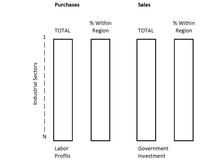
Assume that we have the necessary funds to survey an appropriately stratified sample (by size and industrial composition) of all the firms within a region. From each firm, we would request information shown in Figure 2.2. The firm would be asked to detail its total purchases of goods (column l) irrespective of the geographic origin of these purchases; similarly, the firm would be asked to specify the industrial sectors purchasing its output (column 3). In addition, the firms would be asked to provide information on purchases of labor and returns to capital (profits, dividends, and taxes) and sales to consumers, government, and for investment purchases. These transactions will be explained in greater detail later on in thenext chapter. As we are dealing with a regional economy, we are going to be interested in the transactions that take place within the region as opposed to those with firms outside the region. For this reason, the firms in the survey would be asked to provide an estimate of their purchases (column 2) and sales (column 4) that occur within the region.

(19)

Figure 2.2 Survey Information Requested from Each Firm

There are a number of major, tricky accounting issues that have to be resolved in order to move from the sample data to an input-output table. These will be mentioned here but not explained in great detail (see

Miernyk,1965). First, some rules have to be adopted to allocate firms to sectors. In the format that will be used in this book, the rule is usually based on the principal product of the firm.2 The number of sectors identified will vary; some models show as few as 10, others as many as 400. Much will depend on the funds available for survey analysis and whether, in fact, survey data can be collected at all.3 Furthermore, flows are usually shown in producers’ rather than purchasers’ prices; this necessitates allocating trade and transportation margins to the appropriate sectors. These margins may be thought of as the "mark-up" that a wholesaler or retailer charges for the service of marketing that they provide. In some cases, this may be a fixed percentage of the cost of the good (e.g., 25 percent). The transportation margins are an estimate of the transportation cost involved in moving a unit value of the commodity from producer to consumer. Hence, the purchase of a good by another sector may be shown as a combination of the purchase of the good and the purchase of the transport service in having the good delivered (see Figure 2.3a). For a purchase by a consumer, the transaction may involve both a wholesale and a retail mark-up (Figure 2.3b). That is why, in input-output models, consumers are shown as purchasing output from industries directly rather than aggregating all their transactions into the retail sector. A final issue revolves around the problem that as we are using asample of firms, what all firms in sectorisay they sell to sectorj may not correspond to what the firms in sectorjsaid they purchased from sectori. Hence, from the survey data, we end up with two matrices.

2_{In other frameworks, a distinction is made between commodities and industries. This avoids many of the problems of} classification articulated here (seeJensen and Hewings,1985for a review).

(20)

The first documents the sales made by firms to all other sectors in the region whereas the second provides information on the purchases made by firms from other sectors. It would be very surprising if indeed theijth

cell of both matrices contained the same value (suitably scaled to reflect the total population from which the sample was drawn). Accordingly, some careful rationalization of these two estimates must be made. This process has sparked a heated debate in the literature (seeGerking,1976,1979a,1979b: Miernyk,1976 1979).

Note: In this example, the consumer purchase would involve four sectors (1) industrial sector producing good, (2) transport service, (3) wholesale, and (4) retail trade.

Figure 2.3 Trade and Transportation Margins

Now, we are ready to assemble the data into the regional input-output model. The format and the associated equation systems will form the subject of the next chapter. Keep in mind two important ideas; namely, the link with the economic base model and the relationship with national accounting systems of the Keynesian type.

(21)

3

THE BASIC REGIONAL INPUT-OUTPUT MODEL

In this chapter, we shall assemble the survey data obtained from our sample of firms into a simple regional input-output table. Once the assembly is complete, we may begin the process of using the table to develop a model for the purposes of multiplier estimation. InChapter 4, some simple applications of the model and multipliers will be provided.

From the sample surveys, we now have assembled four matrices, one showing purchases made by firms from other firms irrespective of geographic origin, and a second one showing the purchases made from firms within the region. The third and fourth matrices display sales data irrespective of destination and within the region. The matrices showing the sales and purchases relations irrespective of origin and those showing those interactions within the region are “arbitraged” into two matrices. This arbitrage process ensures that consistency of estimation is obtained; it usually involves reconciliation of one or more estimates of the flows between two sectors. Because we are dealing with a system in which total inputs for all sectors equals total outputs for all sectors, any adjustments in the entries in one part of the matrix will require some adjustment to a number of other entries to ensure that balance is maintained. The first matrix (showing total transactions irrespective of origin) approximates what may be referred to as a total technology matrix, whereas the one that only details the transactions within the region is regarded as a regional transaction matrix. In the analysis that follows, most of our attention will be focused on the latter matrix. The transactions that involve purchases from outside the region are usually aggregated into one- or two-row vectors; a distinction is sometimes made between imports from other regions within the country and those from outside the country. The row vector or vectors are placed within the accounting system so that the extraregional transactions are not lost!

3.1

Elements of the Input-Output Table

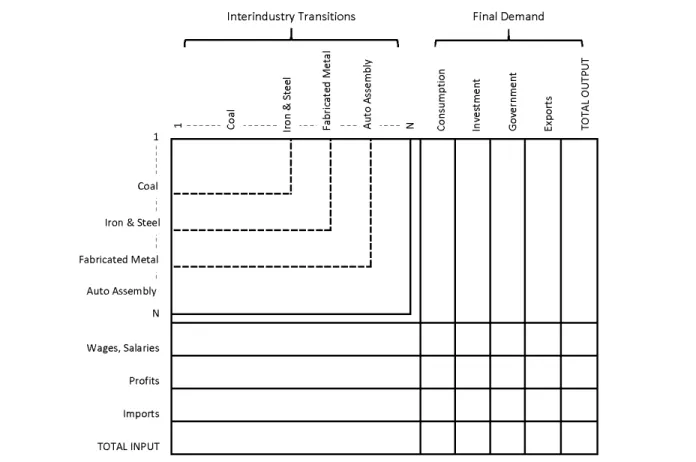
Figure 3.1 shows the general accounting framework: then×nsquare matrix shown in the double-lined box is known as the regional interindustry transactions matrix. A typicalrow,i, in this matrix shows the sales made by industryi to all other industries in the region; a typical column,j, shows the purchases made by this industry from all other industries in the region. What are these flows? They are sales and purchases made on current account and represent stages in the processing ofintermediate goods. Current account purchases are those that a firm needs for the production of its commodities in any given year. Intermediate goods are those that are sold to other firms for further processing prior to sale to consumers. Examples would be sales of coal to an iron and steel plant (cellCSin Figure 3.1 ), sales of rolled steel to a fabricated metal plant (cellSF), sales of automobile bodies to an automobile assembly plant (cellBA), and so forth. However, the sale of a finished automobile to a consumer would not be shown in this part of the matrix. Where will this be found? To the right of the double-lined matrix is a box labeled "Final Demand." In this category are included the purchases by consumers, governments (local, state, and federal), and sales to other activities of investment goods.4. The last category of final demand--exports--picks up the sales made by firms to purchasers outside the region and outside the country. Hence, in parallel to the treatment of imports, two categories of export demand are shown in Figure 3.2--interregional and foreign. If we sum across the ith _{adding the sales to other}

indus-tries and to the various categories of final demand, we arrive at the totalgross outputfor that industrial sector.

4_{Investment goods are those products that are usually regarded as depreciable items, such as a machine, that the purchaser} will depreciate over some finite time span greater than one year.

(22)

Figure 3.1 Schematic Input-Output Table

Now examine the purchases made outside the square matrix in thejth_{column. The category known as value}

added contains two important elements: (1) returns to capital--such as profits and dividends; and (2) returns to labor, namely wages and salaries. Below that are the two import row vectors and finally, a vector of total

gross inputs. One of the major contributions Leontief provided was the so-called "doubleentry" accounting framework shown here; the vectors of total gross output and input are equal. Confronted with this fact, one might comment that if purchases and sales are equal, why are there firms in business? The answer lies in the fact that input-output accounting systems follow standard firm-level accounting balance sheets: total assets and total liabilities are equal for a firm. In input-output analysis, profits are contained within the value-added entry and hence, the system represents a relatively complete picture of the transactions in an economic system. Note that for a transaction to be recorded, an exchange has to take place in themarketplace. Transactions that take place on the "black market" or in the "underground economy" are not recorded here; in developing economies these transactions could amount to a significant percentage of the total volume.

(23)

To:

1 2 3 4 5 6 7 8 9 10 11 12 13 14

Total

Inter Non- Inter-l Total Iron/ Electrical Business Trans- mediate Defense Defense regional Foreign Final Total From Mining Steel Engineering Services portation sales Households State Federal Exports Exports Demand Output

1. Mining 21 - 9 3 - 33 30 10 5 - 20 2 67 100 2. Iron/steel 1 8 7 29 - 45 25 5 2 - 15 8 55 100 3. Electrical engineering 3 20 - 50 7 80 5 1 4 4 3 3 20 100 4. Business services 31 2 38 - 3 74 12 2 - 11 1 - 26 100 5. Trans-portation 10 25 26 1 4 66 9 6 - 13 4 2 34 100 6. Total inter-mediate purchases 66 55 80 83 14 298 81 24 11 28 - -7. Value added 20 40 10 17 40 - 2 49 4 9 - -8. Inter-regional imports 7 4 4 - 30 - 47 18 - 21 - -9. Foreign imports 7 1 6 - 16 - 30 2 - 14 - -10. Total input 100 100 100 100 100 - 160 93 15 72 -

-Figure 3.2 Regional Input-Output, 1984 (producers pricers, $millions)

3.2

Links with National Accounts

Richardson(1972) has provided the link between this format and the national accounting framework articulated inChapter 2. To accomplish this link, some variables need to be defined: Let Xij be the flow of commodities

from industryito industryj on current account;fikis the flow of commodities from industryito categoryk

of final demand (this might be consumption or government for example);vmj is the purchases from value

added categorymby industryJ, andXi is the total input (output) for sectori. The variablesv andf may

be disaggregated as follows:

vj =Pj+Wj (3.1)

fi=Ci+Gi+Ii+Ei (3.2)

where P and W represent profits and wages and salaries and C, G, I, and E are consumer, government, investment, and export sales. Thus, we may now write the row and column balances:

X j Xij+Ci+Gi+Ii+Ei=Xi (3.3) X i Xij+Pj+Wj+Mj=Xj (3.4)

In this case, we have aggregated both types of imports and both types of exports into one category each, namely,M andE. If equations 3.3 and 3.4 are summed over alli andj sectors, we have:

X i X j Xij+Ci+Gi+Ii+Ei= X i Xi (3.5) X j X i Xij+Pj+Wj+Mj= X j Xj (3.6)

It was noted earlier that the vectors of total input and output were equal; hence, the right-hand sides of equations 3.5 and 3.6 are equal. This provides for the expression:

X i X j Xij+Ci+Gi+Ii+Ei= X j X i Xij+Pj+Wj+Mj (3.7)

(24)

Again, note that the interindustry transactions,P i P j Xij andP i P j

Xij, are contained on both sides of the

equation; they are obviously equal and hence drop out. If we defineC, G, I, E, P, W, andM as the vectors representing the variable elements in equation 3.7, we now have:

C+G+I+E=P+W+M (3.8)

Rearranging, we have:

C+G+I+E−M =P+W (3.9)

The left-hand side should look familiar: It is gross national product, whereas the right-hand side is gross national income. In the input-output framework, total final demand equals total value added plus imports. The latter two categories are known together as primary inputs. Thus, we have a strong link between national product and income accounts and the input-output model. Why are interindustry transactions ignored? Essentially, because their inclusion would amount to double-counting: The volume of flows or the number of intermediate transactions are not the major issue--rather, the amount of value created at each stage of production is of importance. This is included in the estimates for gross national product. Clearly, we can appreciate that at the regional level a comparable set of calculations will yield an estimate of gross regional product.

3.3

Regional Input-Output Model

Figure 3.2represents the transactions table for a simple, hypothetical economy: To simplify analysis, each industry is shown to have an output of $100 million. (There is no economic reason for this; in reality, the variation in levels of output will be substantial.) The comparison withFigure 3 .1reveals that interindustry transactions that occur within the region constitute $298 million out of the total output (input) of $500 million; however, the variations by industry are rather large. For example, industry 1 sells only $33 million to other sectors, whereas sector 3 sells $80 million. Similar variations may be seen in terms of purchases from other sectors.

Figure 3.2represents an input-output table for a regional economy; our next task is to convert this to an analytical model. Let us aggregate the entries in columns 7 through 12 of final demand into one column (i.e., column 13); calling this entryfi. Equation 3.3may now be written:

X

X_ij0 +fi=Xi (3.10)

The termX0 will be explained below. We will now make a number of important restrictive but necessary assumptions. First, assume that the demand for inputs is independent of the level of output. By this, we mean that the "recipe" for production (the percentage of total inputs required from each industry) does not vary with the scale of production. Second, the production system is such that no substitutions may be made. Hence, the proportionate use of inputs cannot be changed. These assumptions allow us to define a technical and a regional input coefficient:

aij =Xij/Xj (3.11)

rij=Xij0 /Xj (3.12)

The coefficientaij represents the cents’ worth of input purchased from sectoriby sectorj per unit of output

of sectorj;rij, on the other hand, provides an estimate of the proportion of theaij purchase that is made

from firms located within the region. Hence, the distinction between the two coefficients lies in the distinction between purchases made irrespective of geographic origin (Xij) and those made from within the region (Xij0 ).

(25)

vary over different levels of production. For the analysis that follows, we will use expression 3.12. Rewriting this in terms ofX_ij0 , we have:

X_ij0 =rijXj (3.13)

Substituting this expression in equation 3.10 yields:

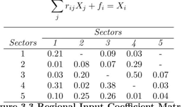
X j rijXj+fi=Xi (3.14) Sectors Sectors 1 2 3 4 5 1 0.21 - 0.09 0.03 -2 0.01 0.08 0.07 0.29 -3 0.03 0.20 - 0.50 0.07 4 0.31 0.02 0.38 - 0.03 5 0.10 0.25 0.26 0.01 0.04

Figure 3.3 Regional Input Coefficient Matrix

Figure 3.3 shows the values for the entries in the interindustry portion of the matrix inFigure 3.2, converted to regional input or regional requirements coefficients. These entries provide the proportion of the total requirements (namely thea_ijs) necessary to make $1 of output in thejthindustry that come from industries within the region. As we have five industrial sectors, there will be five equations of the type shown in equation 3.14. In matrix terms, the system may be set up as follows:

      r11 r12 r13 r14 r15 r21 r22 r23 r24 r25 r31 r32 r33 r34 r35 r41 r42 r43 r44 r45 r51 r52 r53 r54 r55             X1 X2 X3 X4 X5       +       f1 f2 f3 f4 f5       =       X1 X2 X3 X4 X5       (3.15)

If we letRbe the 5×5 matrix ofrijs;X the 5×1 vector of total outputs (inputs) andf the 5×1 vector of

final demands, equation 3.15 may be written in a more compact form that we may solve the simultaneous system in a more efficient manner.

RX+f =X (3.16)

If equation 3.16 is rearranged and factored, a solution forX may be derived:

f =X−RX

= (I−R)X

(I−R)−1f =X (3.17)

where I is an identity matrix, a matrix with the value 1 along the main diagonal and zero elsewhere. If equation 3.15 is examined, it will be clear that the production of output in each industry theoretically involves the purchases of inputs from all other industries. In reality that will not be the case; an examination of Figure 3.3 reveals that sector 2 makes no purchases from sector 1 and sector 5 has no direct needs from

(26)

sectors 1 and 2.5 However, this should not be interpreted as implying that these sectors are not linked at all; the operative word here is thedirect linkage. As we shall see later, firms that are not linked directly may be linked indirectly. For example, note that sector 2 makes no purchases from sector 1 but does purchase inputs from sector 3. This sector, 3, purchases inputs from sector 1. Hence, if the output of sector 2 expands, sector 1 will benefit in the second round of purchases. This may be shown diagrammatically in Figure 3.4. Note that the interactions become very complex and interwoven as the various rounds of spending and re-spending evolve. The analogy with the operation of the consumption effects in Figure 2.1should be clear; after all, equation 3.17 can be rewritten:

(I+R+R2+R3+R4. . . .)f =X (3.18)

Figure 3.4 Rounds of Spending Imports for Sector 2

5_{The entries in cells (1,1), (2,2), and (5 ,5) represent transactions among firms}_within_{an industry. Because our sectors are} very highly aggregated, it is possible that some inter mediate, unfinished goods will be traded with firms that are classified as part of the same sector. In input-output tables with very large numbers of sectors the diagonal elements tend to be very small.

(27)

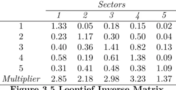
The various expressions ofR represent the rounds of spending taking place in the economy; becauseRis a coefficient matrix,Rt→0 ast→ ∞, wheretdenotes the spending round. Hence, the contribution of each succeeding round diminishes. This part of the equation system in equations 3.18 and 3.17 is thus the direct analogy with the multiplier articulated inChapter 2. In input-output models, it is known as the Leontief Inverse Matrix or the Matrix Multiplier. The values for the regional example are shown in Figure 3.5. These entries provide the total requirements within the region for each industry to deliver $1 worth of output to final demand. Our suspicions that sectors might be linked indirectly is well illustrated here. As a result of all the transactions in the economy, note that sector 2 purchases 0.05 cents worth of output from sector I in order to make a delivery of $1 to final demand.

Sectors 1 2 3 4 5 1 1.33 0.05 0.18 0.15 0.02 2 0.23 1.17 0.30 0.50 0.04 3 0.40 0.36 1.41 0.82 0.13 4 0.58 0.19 0.61 1.38 0.09 5 0.31 0.41 0.48 0.38 1.09 Multiplier 2.85 2.18 2.98 3.23 1.37

Figure 3.5 Leontief Inverse Matrix

What is the direct relationship of the entries in Figure 3.5 to the multipliers noted inChapter 2? If the entries in a typical column of Figure 3.5 are summed, we have what is known as the output or column multiplier. Unlike the economic base model or the Keynesian system, we now have a multiplierfor each industry. These are shown in the last row of Figure 3.5. Note that they vary rather substantially from one sector to another; hence, the use of an aggregate multiplier in an economic base model may provide a somewhat misleading impression of the likely impacts of any change in external demand on the regional economy. The reasons for these variations may be ascribed to (1) the degree to which industrial sectors are linked with each other (i.e., the number of nonzero entries in the matrix of interindustry transactions) and (2) the strength of those linkages (i.e., whether the linkages between sectors are of the same order of magnitude or dominated by one or two very large linkages). InFigure 3.3, one can see that sector 5 makes purchases from two other sectors (apart from itself) and these are not very large amounts. Accordingly, it has the lowest multiplier. Sector 4,

on the other hand, is more intensely linked with the rest of the economy and has the largest multiplier. At this stage, it would be erroneous to equate the size of the output multiplier with the importance of that sector in the regional economy. The multiplier tells us nothing about the level of sectoral output or its importance in terms of employment generation or income formation. We will deal with these issues in the next section.

3.4

Income and Employment Multipliers

Not only do industries make purchases from other sectors, they also mark purchases from the labor force. The next task is to calculate the various income multipliers associated with these purchases; there are three and possibly more types of income multipliers that can be obtained. In this section, we will restrict ourselves to the two most commonly identified, namely, the Type 1 (direct and indirect) and the Type 2 (direct, indirect, and induced). To do this, we will first derive an additional row of coefficients, these being the entries shown in row 7 ofFigure 3.2. Assume for the moment that all the entries in the value added row are for wages and salaries. If these entries are divided by the relevant sectoral output, we can obtain a vector showing cents worth of labor input per unit of output. This is shown below:

Sector Number 1 2 3 4 5

Input of Labor 0.2 0.4 0.1 0.17 0.4

Here we see rather substantial differences in the purchases of labor by sector. These entries will now be represented by a row vectorV. If this vector is multiplied against the Leontief Inverse matrix, we will obtain

(28)

a matrix of direct and indirect income changes:

V(I−R)−1 (3.19)

If these entries are then divided by the direct income changes, V, we have what is known as the Type 1 Income Multiplier (M1):

M1 =V(I−R)−1Vˆ −1 (3.20)

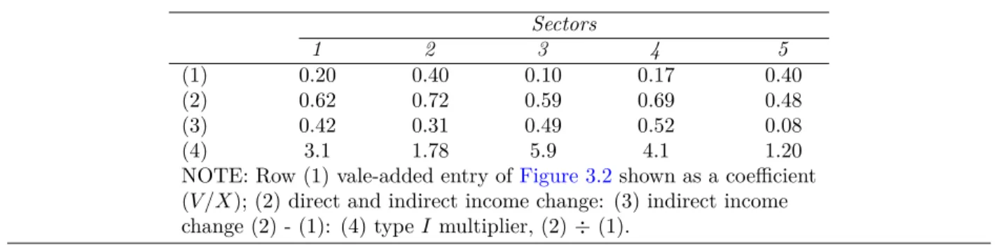
Where the ˆ indicates a vector expressed as a diagonal matrix. The procedure may be demonstrated with reference to sector 1; each entry in the first column of Figure 3.5 will be multiplied by the corresponding row entry detailing the labor input per unit of output (shown as the first row of Figure 3.6).

Sectors 1 2 3 4 5 (1) 0.20 0.40 0.10 0.17 0.40 (2) 0.62 0.72 0.59 0.69 0.48 (3) 0.42 0.31 0.49 0.52 0.08 (4) 3.1 1.78 5.9 4.1 1.20

NOTE: Row (1) vale-added entry of Figure 3.2shown as a coefficient (V /X); (2) direct and indirect income change: (3) indirect income change (2) - (1): (4) typeI multiplier, (2)÷(1).

Figure 3.6 Leontief Inverse Matrix

1.33×0.20 = 0.26 0.23×0.40 = 0.09 0.40×0.10 = 0.04 0.58×0.17 = 0.09 0.31×0.40 = 0.12 Total = 0.62

The summation above may not equal 0.62 exactly because of rounding error; the results of this manipulation for all sectors are shown in Figure 3.6. Again, caution should be exercised in ascribing importance to size in terms of multiplier values. A sector with a large entry inV and with a high level of output may offset the fact that its income multiplier may be relatively small. Because industries 3 and 4 are so highly linked in the system, their indirect income effects are very large in comparison to the direct income effects—hence, the income multipliers are very large.

The income picture is not really complete because we have not taken into account the fact that wages and salaries received by local employees may be spent on local goods and services, thereby generating additional output and, hence, additional income. There are a number of ways in which these effects can be calculated. The most direct way is to expand or augment the direct coefficients’ matrix (Figure 3.3) to include the additional rowV that we have already defined and an additional complementary column. This column is the vector of consumption coefficients by sector; in a sense, it represents a disaggregation of the average propensity to consumer by all households in the region (i.e., column 7 of hyperlinkfigure3.2Figure 3.2). This consumption is restricted to the output of goods and services produced within the region; imports are shown in rows 8 and 9 of column 7 ofFigure 3.2. The augmented matrix (R0) is shown in Figure 3.7; the solution is now obtained in a similar way, except thatf0 does not contain the consumption account:

(29)

Sectors HH 1 2 3 4 5 6 1 0.21 - 0.09 0.03 - 0.18 2 0.01 0.08 0.07 0.29 - 0.15 3 0.03 0.20 - 0.50 0.07 0.03 4 0.31 0.02 0.38 - 0.03 0.07 5 0.10 0.25 0.26 0.01 0.04 0.05 HH 6 0.20 0.40 0.10 0.17 0.40 0.01

Figure 3.7 Expanded Matrix

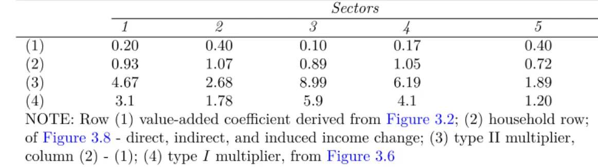
The multiplier matrix, (I−R0)−1_{, is shown in Figure 3.8. Type 2 income multipliers,}_M_{2, are simply the}

division of the household row entries of the augmented Leontief Inverse of Figure 3.8 by the direct income entries, V. These are shown in Figure 3.9 together with a comparison with theM1 multipliers. Several authors have noted, and subsequently proved, that, for any matrix, there is a constant relationship between theM1 andM2 multipliers. As this constant can be derived without the inversion of the augmented matrix, once theM1 multipliers are known, the M2 values can be calculated rather easily. (For a proof, seeMiller and Blair,1985, p. 143.) Sectors HH Sectors 1 2 3 4 5 6 1 1.59 0.34 0.43 0.43 0.21 0.41 2 0.48 1.46 0.54 0.78 0.23 0.41 3 0.62 0.61 1.62 1.07 0.30 0.36 4 0.82 0.47 0.84 1.65 0.28 0.39 5 0.52 0.65 0.68 0.62 1.25 0.34 HH 6 0.3 1.07 0.89 1.05 0.72 1.50

Figure 3.8 Leontief Inverse Matrix with Households Endogenous

Sectors 1 2 3 4 5 (1) 0.20 0.40 0.10 0.17 0.40 (2) 0.93 1.07 0.89 1.05 0.72 (3) 4.67 2.68 8.99 6.19 1.89 (4) 3.1 1.78 5.9 4.1 1.20

NOTE: Row (1) value-added coefficient derived fromFigure 3.2; (2) household row; ofFigure 3.8- direct, indirect, and induced income change; (3) type II multiplier, column (2) - (1); (4) typeI multiplier, fromFigure 3.6

Figure 3.9 Derivation of Type II Multipliers and Comparison with Type I

A final note on income multipliers should be made; incomegenerated within a region may not be equal to incomeretained and then spent in the region. Labor force commuting across regional boundaries, repatriation of income to other regions and various taxation levies applied by state and national governments may all serve to reduce the size of the income pool expended in the region. On the other hand, additional non-wage and salary income (dividends, interest payments, and government transfers) may enhance the pool of income earned from employment. These accounting issues have been addressed in many recent more sophisticated regional social accounting models (seeBatten and Andersson,1983, for an example).

Finally, if we assume that the levels of employment in an industry are closely related to output, such that an employment/output ratio can be defined for all levels of output, then the entries in the input-output system

(30)

can be converted to employment terms to yield employment multipliers. The procedure is as follows; rewrite equation 3.10in matrix form:

X0i+f =X (3.22)

where X0 is the matrix of interindustry flows within the region and I is an identity vector that we use to sum across the rows of matrixX0. Ifeis defined as the employment vector showing employment by sector, then the expressioneX−1 _{provides the employment output ratios (number of jobs per $million of output). If all}

the entries in equation 3.22 are multiplied by this expression, we have:

ˆ

eXˆ−1X0i+ ˆeXˆ−1f = ˆeXˆ−1X (3.23) The right-hand side becomese, becauseX−1X is equal to the identify matrix; that fact can also be used to replaceion the left-hand side withe−1e. Hence, we now have:

ˆ

eXˆ−1X0ˆe−1e+eXˆ−1f =e (3.24) Factoring and simplifying, we have:

ˆ

eXˆ−1f =e−eˆXˆ−1X0eˆ−1e

= (I−ˆeXˆ−1X0eˆ−1)e

(I−eˆXˆ−1X0eˆ−1)−1eˆXˆ−1f =e (3.25) The inverse matrix in equation 3.25 is the direct analogy to the Leontief inverse matrix in dollar terms; all the entries are now expressed in employment terms. Given a change in final demand, we can determine the level of employment required, directly and indirectly, in each industry. The expression ˆeXˆ−1X0ˆe−1 converts the cents per dollar coefficient matrix shown inFigure 3.3into one showing employment coefficients,eijs, the

employment required from industryiper employee in industryj to support output in industryj.

3.5

Summary

Now that the conversion of the input-output table to a model has been demonstrated, the model can be used for analytical purposes. The reader should be wary of inferring to much from the rankings of employment and income multipliers. For example, many labor-intensive sectors have low employment multipliers simply because the denominator of the multiplier (the direct effects) is relatively large. In absolute terms, though, these sectors may generate the largest volume of employment. In the next chapter, some simple examples will be provided prior to some discussion about the ways in which an input-output model might be constructed from other than survey data. Chapters 6 and7will extend this simple, single-region framework spatially (into the interregional context) and sectorally (by specifying different income groups, different types of labor

(31)

4

APPLICATIONS

Now that an input-output table has been developed from the survey data and the input-output model, we can use the system to undertake some relatively straightforward applications of the model. In this chapter, two illustrations will be provided; the first examines the impact on employment and output of a change in a federal government’s programs. For example, we might wish to consider the effects of a shift away from defense to social programs. The second example shows how the input-output model might be used to undertake a cost-benefit analysis of a project. Prior to the discussion of these in-depth examples, some comments will be made on the range of regional input-output applications.

The early applications of regional input-output analysis focused almost exclusively on impact analyses, for example, the effects of government programs on a regional economy. More creative uses were found--for example, the impact of sports franchises on metropolitan economies, the employment and income generated by large institutions such as universities, and the impacts of new transportation facilities on regional economies. Increasing interest in resource scarcity, and environmental and energy problems fostered a whole new series of applications for input-output models. In many cases, the regional models were linked with other analytical systems or recast to provide more flexible forms of analysis. Within these categories, one finds applications of air pollution abatement programs, the effects of water shortages on regional economic growth, and development and many applications exploring the effects of disruptions in energy supply on various regional economic indicators.

Regional input-output models have been used for policy simulation, for forecasting employment, output and income, and as components in integrated modeling ventures. A great deal more detail is provided in

Miller and Blair(1985), especially on the applications of input-output analysis in the solution of energy and environmental problems.

4.1

Impact Analysis with an Input-Output Model

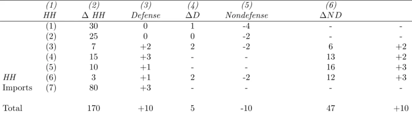
Let us assume that the federal government is considering a cut of $10 million in defense spending in the regional economy and reallocating the funds either to a non-defense-oriented set of programs (e.g., social welfare, education) or to consumers in the form of a reduction in taxes. Hence, in the first case, government expenditure in the region will remain the same ($10 million). Should one therefore conclude that the net impact on the region’s economy will be zero? lf we had been working with a simple economic base model, that would have been a correct assertion. However, even though the total expenditure by the federal government in the region will remain the same, the impacts will not necessarily be identical. The reasons lie in the differences in theallocationby sector of the two budget reallocations in comparison with the original defense-related expenditure. It is unlikely that the same goods and services will be needed to support a defense program as will be needed for a social welfare program or the consumption needs of local consumers. For this reason, we should not expect similar impacts from the reallocation from defense to consumer spending even though, once again, the total amount of final demand being allocated in the region is the same.

(1) (2) (3) (4) (5) (6) HH ∆HH Defense ∆D Nondefense ∆N D (1) 30 0 1 -4 - -(2) 25 0 0 -2 - -(3) 7 +2 2 -2 6 +2 (4) 15 +3 - - 13 +2 (5) 10 +1 - - 16 +3 HH (6) 3 +1 2 -2 12 +3 Imports (7) 80 +3 - - - -Total 170 +10 5 -10 47 +10

NOTE: Imports rows of Figure 3.2 have been combined, HH, households; D, defense; ND, nondefense.

(32)

Figure 4.1 shows the reallocation of final demand from defense to nondefense and from defense to households. In the allocation to households, not that the $10 million was not distributed proportionately to the original vector of expenditures. Empirical evidence suggests that consumers allocateadditionsto income differently than theiraverageincome. Thus, although the original vector might be regarded as an expression of average propensities to consume, the distribution of the $10 million is assumed to follow the dictates of a vector of marginal propensities to consume. Similarly, the vector of additions to nondefense spending reflects a slightly different reallocation from the existing distribution, although one that is not as significantly different in appearance as those between the average and marginal propensities to consume by households.

Figures 4.2 and 4.3 show the results of the impact analyses; using the employment/output ratios shown in Figure 4.2, the employment impacts were also calculated as well as the output effects. As we suspected earlier, even though the total amount of money being spent by the various sectors of final demand was unchanged, the reallocations severely altered the outcomes on a sector-by-sector basis. The gross effects are shown in Figure 4.2 and the net effects are summarized in Figure 4.3. Sectors 4 and 5 were net gainers from a reallocation to either households or nondefense spending, whereas sector 3 gained from the household but not the nondefense reallocation. Sectors l and 2 would suffer losses from both reallocations. Because the employment data are linearly dependent on the output figures, these results hold for both employment and output. The magnitude of the changes varied by sector rather appreciably. Notice that sector 5 gained far more from a nondefense reallocation than from a consumer spending addition; in part, this is due to the fact that $3 million of the reallocation would be "lost" to the regional economy if added to consumers’ income by reason of import purchases. The overall effects led to decreases in available jobs in the region and a loss of production. Several comments need to be made here; first, no consideration is given to the possibilities that some sectors may not be able to adjust their production from defense to nondefense or consumer goods instantaneously. Second, the employment data reflectaverageemployment/ output ratios; some sectors may be able to produce less output by curtailing employment opportunities in a greater than proportionate manner, thus creating additional layoffs. Third, nothing is revealed in this analysis about the various skill categories required; for some occupations, the demand for their skills may actually arise during a reallocation, whereas for others the demand may be drastically reduced. Hence, the overall employment impacts may hide significant dislocations and disequilibria in supply-demand relationships.

Employment Decrease Defense Increase Nondefense Increase Household per $1 Million

Sectors Output Employment Output Employment Output Employment Output

1 - 5.78 -1056 + 0.72 + 154 + 0.83 + 166 200 2 - 3.86 -1930 + 1.72 + 860 + 2.14 +1070 500 3 - 5.14 -1542 + 4.85 +1455 + 5.41 +1623 300 4 - 3.90 -1950 + 4.25 +2125 + 5.45 +2725 500 5 - 3.02 -1208 + 4.99 +1996 + 3.19 +1276 400 Total($) -21.70 -7686 +16.53 +6590 +17.02 +6860

Figure 4.2 Employment and Output Effects of Changes in Final Demand

Defense to Nondefense Defense to Household Sectors Output Employment Output Employment

1 -5.06 - 902 -4.95 -890 2 -2.14 -1070 -1.72 -860 3 -0.29 - 87 +0.27 + 81 4 +0.35 + 175 +1.55 +775 5 +1.97 + 788 +0.17 + 68 Total($) -5.17 +1096 -4.68 -826

(33)

A final word of caution: one should not infer from this analysis that defense spending is essential to the maintenance of regional economic vitality. This example uses data that may or may not reflect reality. Furthermore, nothing is revealed about the possible longer-run implications of such changes. Some local firms, faced with declining demand, may make some changes in their production process or product lines in the hopes of securing new markets within the region and elsewhere. The input-output model cannot hope to answer all the questions related to impacts of the kind demonstrated here. One major effect not considered, of course, is the role of migration. In regional economies, downturns and upswings in the business cycle can have pronounced effects on the volume of in- and out-migration. The expectations on the part of individuals, with respect to the duration of unemployment, also with respect to the duration of unemployment will also play a critical role in the “mover/stayer” equation. However, the sectoral detail afforded by the input-output model does provide an important source of information not available from other, more aggregated methods of regional analysis. Similar studies can be undertaken, for examp1e, to measure the impact of a new firm (even a sports franchise) on a regional economy or the effect of the closure of an existing plant. In the latter case, the mobility of the newly unemployed workers will play a crucial role in maintaining the remaining levels of activity in the region. This issue will be addressed inChapter 7.

4.2

Using an Input-Output Model in Project Appraisal

In many economies, one of the more important objectives associated with economic development is the need to narrow the differences in welfare between regions. In a number of cases, the index used for comparison is the level of income per capita. Achieving this goal requires careful selection of policy instruments designed to steer allocation of resources in such a way that the less prosperous regions receive some possibility for improving their welfare at a faster rate than the more prosperous regions. The choice of these policy options would form the subject of another monograph and will not be considered here; let us assume that the country in question has decided that the availability of large supplies of coal in the region might provide an opportunity for the penetration of markets in other regions and other countries, especially in the face of rising petroleum prices. However, the project will require some initially large capital investment in machinery; transportation systems, and so forth. Can the project be justified? If we restrict ourselves to economic issues, cost-benefit analysis can be used to help answer the question about the wisdom of this project vis-à-vis several others. The linkage of input-output models with cost-benefit appraisal techniques was first suggested byTinbergen(1966) and has subsequently been utilized in a number of different contexts (seeKuyvenhoven,

1978;Karunaratne, 1976; and for a regional application Bell et al.,1982).

(34)

Total initial Demand Change*

Mining .21 .0 .09 .03 .0 15

Iron & Steel .01 .08 .07 .29 .0 0

Elec. Eng. .03 .20 .0 .50 .07 0 Bus. Ser. .31 .02 .38 .0 .03 0 Trans. .10 .25 .26 .01 .04 0 V .2 .4 .1 .17 .4 K .13 .15 .10 .05 .10 [I−RN N<