Deep Neural Network for Tra
ffi
c Sign Recognition Systems: An
analysis of Spatial Transformers and Stochastic Optimization
Methods
´
Alvaro Arcos-Garc´ıa⇤, Juan A. ´Alvarez-Garc´ıa, Luis M. Soria-Morillo Dpto. de Lenguajes y Sistemas Inform´aticos, Universidad de Sevilla, 41012, Sevilla, Spain
Abstract
This paper presents a Deep Learning approach for traffic sign recognition systems. Several classification experiments are conducted over publicly available traffic sign datasets from Germany and Belgium using a Deep Neural Network which comprises Convolutional layers and Spatial Transformer Networks. Such trials are built to measure the impact of diverse factors with the ultimate goal of designing a Convolutional Neural Network that could improve the state-of-the-art of traffic sign classification task. On one hand, di↵erent adaptive and non-adaptive stochastic gradient descent optimization algorithms such as SGD, SGD-Nesterov, RMSprop and Adam are evaluated. On the other hand, multiple combinations of Spatial Transformer Networks placed at distinct positions within the main neural network are analysed. The proposed Convolutional Neural Network reports a recognition rate accuracy of 99.71% in the German Traffic Sign Recognition Benchmark, outperforming previous state-of-the-art methods and also being more efficient in terms of memory requirements.
Keywords: deep learning, traffic sign, spatial transformer network, convolutional neural network
1. Introduction
Traffic sign recognition systems (TSRS) are essential in many real-world applications such as autonomous driving, traffic surveillance, driver safety and assistance, road network maintenance or urban scene understanding. Normally, a TSRS concerns two related subjects which are traffic sign detection (TSD) and traffic sign recognition (TSR). The former focus on the localisation of the targets in the pictures while the later performs a fine-grained classification to identify the type of the detected targets (De La Escalera et al., 1997).
Traffic signs are a fundamental asset within the road network because their aim is to be easily noticeable by pedestrians and drivers in order to warn and guide them during
⇤Corresponding author.
Email addresses: [email protected]( ´Alvaro Arcos-Garc´ıa),[email protected](Juan A. ´Alvarez-Garc´ıa), [email protected](Luis M. Soria-Morillo)
Manuscript
both day and night time. The fact that signs are designed to be unique, rigid and to have distinguishable features such as simple shapes and uniform colours implies that its detection and recognition is a constrained problem. Nevertheless, the development of a robust real-time TSRS is still a challenging task due to real-world variability such as scale variations, bad viewpoints, motion-blur, faded colours, occlusions or lightning conditions. On top of that, there are more than 300 di↵erent traffic sign categories defined by the Vienna Convention on Road Traffic (United Nations Economic Commission for Europe, 1968). This treaty has been signed by 63 countries though there still exists minor visual variations of traffic sign pictographs between countries which can lead to demanding tasks for a machine. Any TSRS must cope well with such issues.
The main contributions of this work are four-fold: (1) A state-of-the-art traffic sign recognition system based on a Convolutional Neural Network (CNN) that includes Spatial Transformer Networks (STN) and outperforms previously published works related with the German Traffic Sign Recognition Benchmark (GTSRB) (Stallkamp et al., 2011). (2) We provide an insight into the proposed CNN capabilities along with the performance impact of spatial transformer layers within the network. (3) Analysis of the e↵ect of diverse gra-dient descent optimization algorithms on the presented CNN. (4) Multiple public available European traffic sign classification datasets are reviewed and evaluated by the CNN. These contributions lead to practical applications such as self-driving cars or automated inventory and maintenance of vertical signage since the CNN can perform fine-grained classification once the traffic sign has been detected. Moreover, as the CNN outperforms the human visual system, its inference time is quite low and also can be deployed as a standalone service, it could be used in real-time applications.
The rest of the paper is organised as follows. Section 2 review related works of traffic sign recognition systems. Section 3 describes the experiments conducted to analyse the impact of both spatial transformers and stochastic optimization algorithms on the proposed CNN. Then, recognition results are shown in Section 4. Finally, conclusions and further work are drawn in Section 5.
2. Related works
Chronologically, approaches of published works on traffic sign recognition systems evolved from colour and shape based methods to machine learning based methods. In recent times, CNNs have attracted attention in pattern recognition and computer vision research, and have been widely adopted for both object detection and recognition.
Colour-based approaches are very common. These methods use di↵erent colour spaces for segmentation of the road image such as RGB (Escalera et al., 1997), HIS (Maldonado-Bascon et al., 2007) or HSV (Shadeed et al., 2003), among others. The shape-based method is another popular approach for traffic sign recognition and detection. Symmetry information of circular, triangular, squared and octagonal shapes are used in (Loy & Barnes, 2004), a radial symmetry detector is proposed in (Barnes et al., 2008), Hough transforms are investigated in (Barnes et al., 2010) and a circular traffic sign recognition system is studied in (Kaplan Berkaya et al., 2016).
One of the main problems before the year 2011 was the lack of a publicly available traffic sign dataset. The Belgian Traffic Sign Dataset (BTSD) (Timofte et al., 2011), the German Traffic Sign Recognition and Detection Benchmark (GTSRB and GTSDB) (Stallkamp et al., 2011), and more recently, the Croatian traffic sign dataset (rMASTIF) (Jurisic et al., 2015), the Dataset of Italian Traffic Signs (DITS) (Youssef et al., 2016) and the Tsinghua-Tencent 100K benchmark (Zhu et al., 2016) solved this issue and boosted the research in TSRS because some of them are commonly used to evaluate the performance of computer vision algorithms for traffic sign detection and recognition.
Mathias et al. (2013) propose fine grained classification applying di↵erent methods through a pipeline of three stages: feature extraction, dimensionality reduction and clas-sification. On GTSRB, they reach 98.53% of accuracy merging grayscale values of traffic sign images and Histogram of Oriented Gradients (HOG) based features, reducing the di-mensionality through Iterative Nearest Neighbours-based Linear Projections (INNLP) and classifying with Iterative Nearest Neighbours (Timofte & Van Gool, 2015) (INNC). Although Support Vector Machines (SVM) (Salti et al., 2015), Random Forests (Zaklouta et al., 2011) and Nearest Neighbours (Gudigar et al., 2017) classifiers have been used to recognise traffic sign images, Convolutional Neural Networks (Lecun et al., 1998), also known as ConvNets or CNNs, showed particularly high classification accuracies in the competition. Cire¸san et al. (2012) won the GTSRB contest (Stallkamp et al., 2012) with a 99.46% accuracy thanks to a committee of 25 CNN by using data augmentation and jittering. Sermanet & LeCun (2011) use multi-scale CNN achieving an accuracy of 98.31%, second place in the GTSRB challenge. Later, Jin et al. (2014) propose a hinge loss stochastic gradient descent method to train an ensemble of 20 CNNs that brought o↵ 99.65% accuracy and o↵ered a faster and more stable convergence than previous works. However, these approaches can still be improved avoiding the use of hand-crafted data augmentation and keeping away from applying multiple CNNs in an ensemble or in a committee way for the reason that it normally leads to higher memory and computation costs.
3. Methodology
In this work, we propose a traffic sign recognition system that carries out fine-grained classification to traffic sign images through a CNN whose main blocks are convolutional and spatial transformer modules. In order to find out an accurate and efficient CNN for such purpose, we research and discuss firstly the e↵ect of the use of several STNs and secondly the results applying di↵erent stochastic gradient descent optimization methods.
3.1. Dataset and data pre-processing
Several public available traffic sign datasets have been gathered in countries like United States (Mogelmose et al., 2012), Belgium (Timofte et al., 2011), Germany (Stallkamp et al., 2011), Croatia (Jurisic et al., 2015), Italy (Youssef et al., 2016), Sweden (Larsson & Felsberg, 2011) and China (Zhu et al., 2016). Since the GTSRB (Stallkamp et al., 2011) is the most used for comparing traffic sign recognition approaches, we focus both the spatial transformer e↵ectiveness and cost function optimization experiments on it.
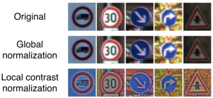
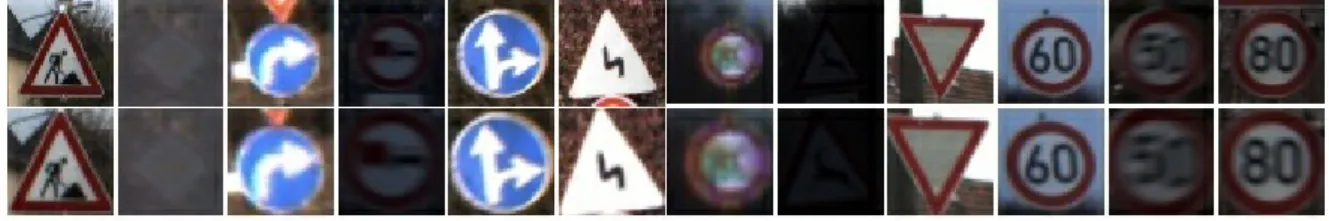
Figure 1: GTSRB dataset pre-processed.
The German traffic sign recognition dataset contains traffic sign samples with di↵erent resolutions that were extracted from 1-second video sequences. They belong to one of the 43 existing classes. Training set has 39,209 images and validation set consists of 12,630 images which are used to measure the performance of algorithms in the GTSRB. Traffic sign samples are raw RGB and sizes vary from 15x15 to 250x250 pixels. During pre-processing stage, all of them are down-sampled or up-sampled to 48x48 pixels and both global normalisation and local contrast normalisation with Gaussians kernels (Jarrett et al., 2009) are computed for the purpose of centring each input image around its mean value as well as enhancing edges (Fig. 1).
3.2. Convolutional Neural Network architecture
Inspired by Cire¸san et al. (2012) approach, the proposed method to recognize traffic signs is a CNN that combines several convolutional, spatial transformer (Jaderberg et al., 2015), ReLU (Nair & Hinton, 2010), local contrast normalization (Jarrett et al., 2009) and max-pooling (Scherer et al., 2010) layers. It acts as a feature extractor that maps raw pixel information of the input image into a tensor to be classified by two fully connected layers. Spatial transformer layers are used to perform explicit geometric transformations on feature maps in order to focus on the object to be learned, removing progressively background and geometric noise. All variable parameters used in each of these layers are optimized together through minimization of the misclassification error over the GTSRB training set.
Spatial Transformer Networks aim to perform a geometric transformation on an input map so that provides to CNNs the ability to be spatially invariant to the input data in a computationally efficient manner. Thanks to such transformations, there is no need for extra training supervision, hand-crafted data augmentation (e.g. rotation, translation, scale, skew, cropping) or dataset normalisation techniques. This di↵erentiable module can be inserted into existing convolutional architectures because the parameters of the transformation that are applied to feature maps are learned by means of a backpropagation algorithm. Spatial transformer networks consist of 3 elements: the localisation network, the grid generator and the sampler (Fig. 2).
The localization network floc() takes an input feature map U 2 RH⇥W⇥C, where H, W
and C are the height, width and channels respectively, and outputs the parameters ✓ of the transformation T✓ to be applied to the feature map ✓ = floc(U). The dimension of ✓
Figure 2: Spatial transformer network components (Jaderberg et al., 2015).
Figure 3: Spatial transformer network. Input images on the left and output images on the right after computing affine transformations.
depends on the transformation type T✓ that is being parameterised, being 6-dimensional in our proposed net as a result of performing a 2D affine transformation A✓ which allows translation, cropping, rotation, scale and skew. The localisation network can comprise any number of convolutional and fully connected layers and must have at least one final regression layer to generate the transformation parameters ✓. Such parameters are used by the grid generator to create a sampling grid, which is a set of points where the input map has to be sampled to obtain the desired transformed output. Finally, the sampler uses as inputs the sampling grid and the input feature map U in order to perform a bilinear sampling which produces the transformed output feature map V 2RH0⇥W0⇥C
, whereH0, W0 are the height
and width of the sampling grid.
For source coordinates in the input feature map (xs
i, yis) and a learned 2D affine
trans-formation matrix A✓, the target coordinates of the regular grid in the output feature map (xt
i, yit) are given as follows (Eq. 1): ✓ xs i ys i ◆ =A✓ 0 @ x t i yt i 1 1 A= ✓11 ✓12 ✓13 ✓21 ✓22 ✓23 0 @ x t i yt i 1 1 A (1)
As regards to traffic sign recognition, spatial transformer networks learn to focus on the traffic sign removing gradually geometric noise and background so that only the interesting zones of the input are forwarded to the next layers of the network (Fig. 3). Up to our knowledge, no peer review work has been published including the spatial transformer unit into a CNN for the traffic sign recognition task.
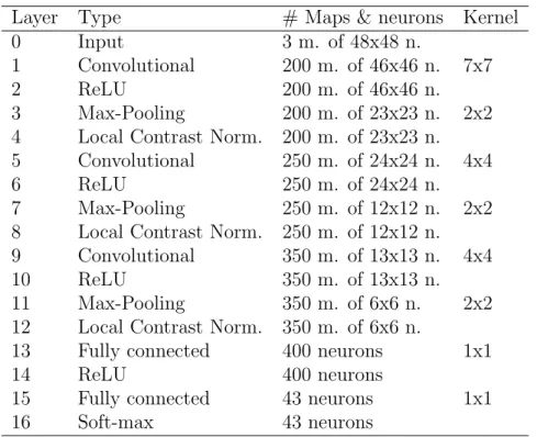
set the main CNN architecture shown in Table 1 that does not contain any STN. Convolu-tional layers’ stride is set to 1 in order to leave all spatial down-sampling computation to max-pooling layers, and zero padding is set to 2. Regarding max-pooling layers, their stride is set to 2 and zero padding to 0. Input and output feature maps of convolutional layers, as well as kernel sizes, are fixed1.
Due to the possibility to combine up to 3 STNs at di↵erent parts of the network, several network architectures were set in order to measure their influence in the final result. Note that the inclusion of more than three STNs are not analysed because output feature maps’ size of following network’s layers could not be further decreased. Progressively, spatial transformer modules are added prior to the convolutional layers of the main network. The localisation network of the three spatial transformer layers is built with a max-pooling layer followed by two blocks of convolutional, ReLU and max-pooling, and finally, two fully-connected layers joined by a ReLU one. The output of the last fully-fully-connected consists of six neurones which correspond to the parameters of the affine transformation matrix. Detailed localization networks architectures are drawn in Table 2. As in convolutional layers configuration, kernel sizes and the number of input and output feature maps are invariable. In total, there are eight di↵erent CNN architectures as a result of the possible combina-tions described. To denote such configuracombina-tions, on one hand,crefers to a convolutional block which includes convolutional, ReLU, max-pooling and local contrast normalisation layers. On the other hand,si indicates thei th configuration of a spatial transformer module. For
instance, a network with just a spatial transformer at the beginning is expressed ass1 c c c.
Note thats1 can only be placed before the first convolutional layer, s2 ahead of the second
convolutional and s3 preceding the third convolutional module.
3.3. Stochastic Gradient Descent Optimization algorithms
Optimization is the process of finding the set of parameters w that minimise the loss function L. The loss function L quantify the quality of a particular set of parameters w based on how well the inferred scores match with the ground truth labels in the training data. In this work, the last layer of the CNNs proposed is a softmax classifier which uses the cross-entropy loss function (Eq. 2) where i enumerates the di↵erent classes, y is the predicted probability distribution and y0 is the true distribution represented as a one-hot
vector. The softmax function (Eq. 3) is used to computey. It takes aK-dimensional vector of arbitrary real-valued scores z and squashes it to aK-dimensional vector f(z) of values in the range (0,1] that sum up to 1 where j represents the j th element of the vectorf.
Hy0(y) = X i yi0log(yi) yi 2(0,1) : X i yi = 18i (2)
Layer Type # Maps & neurons Kernel
0 Input 3 m. of 48x48 n.
1 Convolutional 200 m. of 46x46 n. 7x7
2 ReLU 200 m. of 46x46 n.
3 Max-Pooling 200 m. of 23x23 n. 2x2
4 Local Contrast Norm. 200 m. of 23x23 n.
5 Convolutional 250 m. of 24x24 n. 4x4
6 ReLU 250 m. of 24x24 n.
7 Max-Pooling 250 m. of 12x12 n. 2x2
8 Local Contrast Norm. 250 m. of 12x12 n.
9 Convolutional 350 m. of 13x13 n. 4x4
10 ReLU 350 m. of 13x13 n.
11 Max-Pooling 350 m. of 6x6 n. 2x2
12 Local Contrast Norm. 350 m. of 6x6 n.
13 Fully connected 400 neurons 1x1
14 ReLU 400 neurons
15 Fully connected 43 neurons 1x1
16 Soft-max 43 neurons
Table 1: Main CNN architecture without spatial transformer modules.
Layer/Type Loc. net of ST 1 Loc. net of ST 2 Loc. net of ST 3
0/Input 3 of 48x48 200 of 23x23 250 of 12x12 1/Max-Pool 3 of 24x24 200 of 11x11 250 of 6x6 2/Conv 250 of 24x24 150 of 11x11 150 of 6x6 3/ReLU 250 of 24x24 150 of 11x11 150 of 6x6 4/Max-Pool 250 of 12x12 150 of 5x5 150 of 3x3 5/Conv 250 of 12x12 200 of 5x5 200 of 3x3 6/ReLU 250 of 12x12 200 of 5x5 200 of 3x3 7/Max-Pool 250 of 6x6 200 of 2x2 200 of 1x1
8/Fc 250 neurons 300 neurons 300 neurons
9/ReLU 250 neurons 300 neurons 300 neurons
10/Fc 6 neurons 6 neurons 6 neurons
Table 2: Localisation network details of spatial transformers used in the basic CNN. Kernel size of convo-lutional layers is set to 5x5 and max-pooling layers to 2x2. The annotation shown in the table is simplified, for instance, 3 of 48x48 stands for 3 feature maps of 48x48 neurons each one.
fj(z) = ezj
PK j=1ezk
(3) Gradient descent is the most common and established algorithm to optimize neural network’s loss function. Iteratively, it computes the gradient of the objective function L with respect to the model’s parameters w and updates them. One of its variants is the mini-batch gradient descent that can be written as follows:
wk+1 =wk ⌘krˇL(wk) (4)
It computes the gradient ˇrL(wk) := rL(wk;xk(i:i+n);y(ki:i+n))) of the loss function L
and performs an update for every mini-batch of n training examples x(i) and labels y(i),
representing ⌘ the learning rate.
To accelerate training, some techniques such as Nesterov’s Accelerated Gradient method (NAG) (Nesterov, 1983) and Polyak’s heavy-ball method (HB)(Polyak, 1964) have been widely used. They can be categorised as stochastic momentum methods.
Adaptive optimization methods are another family of gradient descent algorithms. In comparison with non-adaptive methods, they perform local optimization choosing a local distance measure constructed from the history of iterates w1, ..., wk. Examples included
in this category are Adaptive Gradient algorithm (AdaGrad) (Duchi et al., 2011), Root Mean Square Propagation (RMSprop) (Tieleman & Hinton, 2012) and Adaptive Moment Estimation (Adam) (Kingma & Ba, 2015).
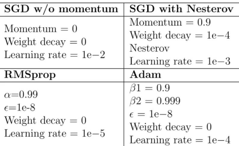
In this paper, we compare the e↵ectiveness of four mini-batch gradient descent optimiza-tion algorithms applied to the CNNs proposed in Secoptimiza-tion 3.2: Stochastic Gradient Descent (SGD) without momentum (Qian, 1999), SGD with Nesterov’s accelerated gradient, RM-Sprop and Adam. For hyper parameter tuning, several networks were trained during few epochs in order to find an adequate initial learning rate value that reaches model conver-gence. We observed that a high learning rate like 0.01 does not work well in the cases of RMSprop and Adam, achieving low accuracy scores. The main reason could be that un-like SGD where learning rate is fixed and optionally it can follow an annealing schedule, RMSprop and Adam calculate adaptive learning rates for each model’s parameter based on the history of iterates. Consequently, a lower learning rate is set for such methods in order to avoid that loss values get stuck at bad spots in the optimization landscape. The initial parameters of these algorithms are shown in Table 3.
4. Results
Once described the CNNs architectures and the loss function optimizers, 32 experiments were run in a computer built with an Intel Core i7-6700k CPU, 16 GB of RAM and a Nvidia Geforce GTX 1070 discrete GPU which has 1920 CUDA cores and 8 GB of RAM, using the Torch scientific computer framework (Collobert et al., 2011) and an implementation of spatial transformer networks for Torch (Oquab, 2017) as development tools. The aim is to find out which are the best places to add the STNs within the CNN at the same time as the
SGD w/o momentum SGD with Nesterov Momentum = 0 Weight decay = 0 Learning rate = 1e 2 Momentum = 0.9 Weight decay = 1e 4 Nesterov Learning rate = 1e 3 RMSprop Adam ↵=0.99 ✏=1e-8 Weight decay = 0 Learning rate = 1e 5 1 = 0.9 2 = 0.999 ✏ = 1e 8 Weight decay = 0 Learning rate = 1e 4
Table 3: Configuration parameters of stochastic gradient descent optimization algorithms.
best stochastic gradient descent optimizer. With a mini-batch size of 50, each experiment is a two-stage process that trains the neural network with the GTSRB training set and then tests it with the GTSRB validation set during 15 epochs. Results draw in Table 4 show the maximum accuracy percentage achieved by each CNN model over the validation set. The best configuration found contains three spatial transformer modules (s1 c s2 c s3 c)
and the computed loss value is optimized by means of SGD without momentum algorithm. On the other hand, worst results are obtained by the CNN that does not include any spatial transformer (c c c) regardless of the optimizer, followed by the CNN with a spatial transformer located right before the last convolutional layer (c c s3 c). It is noteworthy that
the winner configuration doubles the number of model’s parameters of the worst CNN. As a consequence, for the SGD without momentum optimization algorithm, the training time per epoch of the CNN with three spatial transformers is 355.05 ± 0.8 seconds while the CNN without any spatial transfEormer takes 212.12 ± 0.1 seconds. Considering such results and that the solutions found by adaptive methods generalise worse than SGD (Wilson et al., 2017), from now on, we choose the CNNs1 c s2 c s3 c(Fig. 4) along with the SGD without
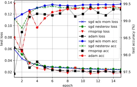
momentum algorithm as our proposed method for traffic sign classification, whose processing time for training and testing one example is 11.18 ± 0.02 and 4.28 ± 0.02 respectively. A comparison of accuracy and loss values computed for each optimization algorithm over the validation set is shown in Figure 5.
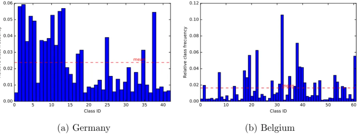
The following subsections describe the German and Belgian traffic sign datasets along with the attained classification results. The structure of each dataset is drawn in Table 5 together with overall recognition results. Note that these datasets are highly imbalanced as can be seen in Figure 6.
4.1. GTSRB dataset results
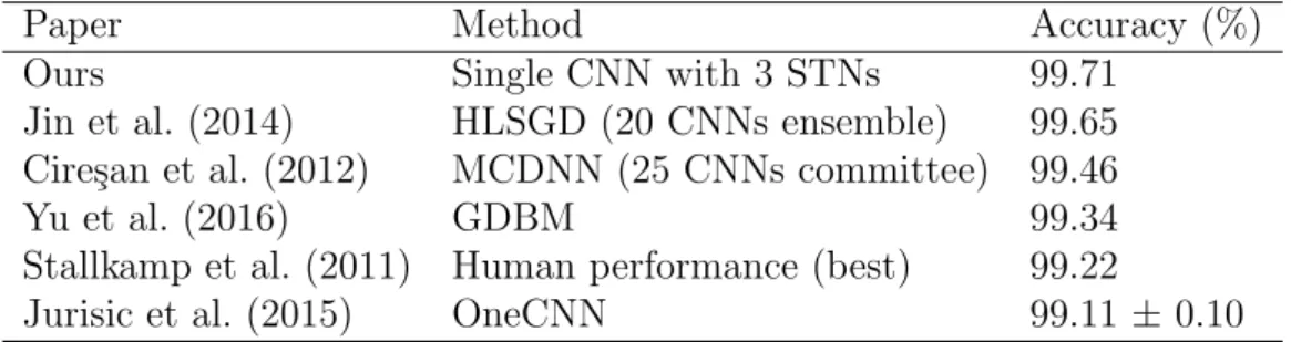
The GSTRB dataset was introduced in Section 3.1. Our proposed CNN with three spatial transformer layers and SGD without momentum as loss function optimizer achieves an accuracy of 99.71% at the 21st epoch (6 more than in the previous experiment). By the time of writing this paper, our method is top-1 ranked in the GTSRB outperforming
CNN/Optimizer SGD SGD-N RMSprop Adam # Parameters c c c 98.31 98.33 98.66 98.81 7,303,883 s1 c c c 99.09 99.15 99.37 99.20 11,137,389 c s2 c c 99.22 99.13 99.28 99.15 9,046,339 c c s3 c 99.02 99.04 99.11 99.39 9,053,839 s1 c s2 c c 99.31 99.30 99.38 99.23 12,879,845 s1 c c s3 c 99.21 99.25 99.32 99.32 12,887,345 c s2 c s3 c 99.34 99.23 99.45 99.28 10,796,295 s1 c s2 c s3 c 99.49 99.43 99.40 99.42 14,629,801
Table 4: Recognition rate accuracy achieved by CNNs configurations described in Section 3.2 using di↵erent loss function optimizers: SGD without momentum (SGD), SGD with Nesterov accelerated gradient (SGD-N), Root Mean Square Propagation (RMSprop) and Adaptive Moment Estimation (Adam). c refers to convolutional block andsto spatial transformer module. Experiments were run during 15 epochs.
Figure 4: CNN for traffic sign recognition. Local contrast normalization layers have been omitted in the figure above to simplify its visualization as well as localization networks of spatial transformers. The st
layers refer to spatial transformer networks, conv to convolutional layers, mp to max-pooling layers,fc to fully-connected layers andsm to soft-max layer.
Figure 5: Comparison of di↵erent loss function optimizers during validation phase applying the CNN model
Dataset Training images Testing images Classes
Germany 39,209 12,630 43
Belgium 4,533 2,562 62
Precision (%) Recall (%) F1 score (%)
Germany 99.71 99.71 99.71
Belgium 98.95 98.87 98.86
Table 5: European traffic sign classification datasets along with precision, recall and f1-score recognition results.
Figure 6: European datasets categories distribution.
Paper Method Accuracy (%)
Ours Single CNN with 3 STNs 99.71
Jin et al. (2014) HLSGD (20 CNNs ensemble) 99.65 Cire¸san et al. (2012) MCDNN (25 CNNs committee) 99.46
Yu et al. (2016) GDBM 99.34
Stallkamp et al. (2011) Human performance (best) 99.22
Jurisic et al. (2015) OneCNN 99.11 ± 0.10
Table 6: Recognition rate accuracy of di↵erent methods on GTSRB.
Paper Data augment.
or jittering
# trainable
parameters # ConvNets
Ours No 14,629,801 1
Jin et al. (2014) Yes ⇠ 23 millions 20 (ensemble)
Cire¸san et al. (2012) Yes ⇠ 90 millions 25 (committee)
Table 7: Proposed CNN’s learnable parameters compared with previous state-of-the-art approaches.
previously published approaches (Table 6). In addition, the total parameters learned by this CNN is 14,629,801 which is much less than in other CNNs proposed for traffic sign recognition systems (Table 7), leading this advantage to lower memory consumption, computational cost and simpler pipeline.
4.2. BTSC dataset results
The Belgian traffic sign classification dataset (BTSC) (Mathias et al., 2013) has 4,533 training images and 2,562 validation ones split into 62 traffic sign types. In comparison with the GTSRB dataset, this one has di↵erent traffic sign pictograms, lighting conditions, occlusions, image resolutions and so on. Moreover, it contains categories that cluster di↵erent traffic signs types (e.g. 50-speed limit sign and 70-speed limit sign) raising the recognition task difficulty. Using the SGD without momentum loss optimizer and the CNN with three spatial transformer layers, the model obtains an accuracy of 98.87% at the 13th epoch (Table 8).
Paper Method Accuracy (%)
Yu et al. (2016) GDBM 98.92
Ours Single CNN with 3 STNs 98.87
Jurisic et al. (2015) OneCNN 98.17 ± 0.22
Mathias et al. (2013) INNLP+SRC(PI) 97.83
5. Conclusions and future work
In this paper, a method for automatic fine-grained recognition of traffic signs is presented. The classification process is carried out by using a single CNN that alternates convolutional and spatial transformer modules. To find out the best CNN architecture, several empirical experiments are conducted in order to investigate the impact of multiple spatial transformer network configurations within the CNN, together with the e↵ectiveness of four stochastic gradient descent optimization algorithms. The CNN model outperforms previous state-of-the-art methods achieving a recognition rate accuracy of 99.71% in the GTSRB, currently top-1 rank. Also, our proposed approach avoids the need of hand-crafted data augmentation and jittering used in prior works (Cire¸san et al., 2012; Sermanet & LeCun, 2011; Jin et al., 2014). Moreover, there are fewer memory requirements and the network has less number of parameters to learn compared with existing methods since we keep away from using several CNNs in a committee or in an ensemble way.
Although our method is ranked on top positions of German and Belgian datasets, there are several recent releases of publicly available traffic sign recognition datasets where it has not been tested due to they were not so established than the previous ones. Nevertheless, up to our knowledge, no scientific paper analyses the use of several STNs and the comparison of stochastic gradient descent optimizers in traffic sign classification problem domain. These experiments and their results can help other researchers to apply to these new datasets.
Future work should study how to build a single deep neural network that could pro-vide top-notch traffic sign recognition rate accuracy in every country whose traffic sign pictographs are quite similar, which is the case of Europe, without needing a particular dataset for each of these countries. Finally, we encourage researchers and companies to build traffic sign classifiers which are robust to adversarial examples as it poses security concerns that could negatively a↵ect, for instance, to self-driving cars, and consequently, the safety of people.
Acknowledgements
This work has been partially supported by the Spanish Ministry of Economy and Com-petitiveness and FEDER R&D through the project ”HERMES – Smart Citizen” (TIN2013-46801-C4-1-R).
References
Barnes, N., Loy, G., & Shaw, D. (2010). The regular polygon detector. Pattern Recognition,43, 592–602. Barnes, N., Zelinsky, A., & Fletcher, L. S. (2008). Real-time speed sign detection using the radial symmetry
detector. IEEE Transactions on Intelligent Transportation Systems,9, 322–332.
Cire¸san, D., Meier, U., Masci, J., & Schmidhuber, J. (2012). Multi-column deep neural network for traffic sign classification. Neural Networks,32, 333–338.
Collobert, R., Kavukcuoglu, K., & Farabet, C. (2011). Torch7: A matlab-like environment for machine learning. InBigLearn, NIPS Workshop EPFL-CONF-192376.
De La Escalera, A., Moreno, L. E., Salichs, M. A., & Armingol, J. M. (1997). Road traffic sign detection and classification. IEEE transactions on industrial electronics,44, 848–859.
Duchi, J., Hazan, E., & Singer, Y. (2011). Adaptive Subgradient Methods for Online Learning and Stochastic Optimization. Journal of Machine Learning Research,12, 2121–2159.
Escalera, a. D. L., Moreno, L., Salichs, M., & Armingol, J. (1997). Road traffic sign detection and classifi-cation. IEEE Transactions on Industrial Electronics,44, 848–859.
Gudigar, A., Chokkadi, S., Raghavendra, U., & Acharya, U. R. (2017). Local texture patterns for traffic sign recognition using higher order spectra. Pattern Recognition Letters, .
Jaderberg, M., Simonyan, K., Zisserman, A. et al. (2015). Spatial transformer networks.Advances in Neural Information Processing Systems, (pp. 2017–2025).
Jarrett, K., Kavukcuoglu, K., Ranzato, M. A., & LeCun, Y. (2009). What is the best multi-stage architecture for object recognition? In 2009 IEEE 12th International Conference on Computer Vision (pp. 2146– 2153).
Jin, J., Fu, K., & Zhang, C. (2014). Traffic Sign Recognition With Hinge Loss Trained Convolutional Neural Networks. IEEE Trans. Intell. Transp. Syst.,15, 1991–2000.
Jurisic, F., Filkovic, I., & Kalafatic, Z. (2015). Multiple-dataset traffic sign classification with OneCNN. In
2015 3rd IAPR Asian Conference on Pattern Recognition (ACPR)(pp. 614–618).
Kaplan Berkaya, S., Gunduz, H., Ozsen, O., Akinlar, C., & Gunal, S. (2016). On circular traffic sign detection and recognition. Expert Systems with Applications,48, 67–75.
Kingma, D. P., & Ba, J. L. (2015). Adam: a Method for Stochastic Optimization. International Conference on Learning Representations 2015, (pp. 1–15).
Larsson, F., & Felsberg, M. (2011). Using Fourier Descriptors and Spatial Models for Traffic Sign Recogni-tion. In Image Analysis Lecture Notes in Computer Science (pp. 238–249). volume 11.
Lecun, Y., Bottou, L., Bengio, Y., & Ha↵ner, P. (1998). Gradient-based learning applied to document recognition. Proceedings of the IEEE,86, 2278–2324.
Loy, G., & Barnes, N. (2004). Fast shape-based road sign detection for a driver assistance system.Intelligent Robots and Systems, 2004. (IROS 2004). Proceedings. 2004 IEEE/RSJ International Conference on,1, 70–75 vol.1.
Maldonado-Bascon, S., Lafuente-Arroyo, S., Gil-Jimenez, P., Gomez-Moreno, H., & Lopez-Ferreras, F. (2007). Road-Sign Detection and Recognition Based on Support Vector Machines. Intelligent Trans-portation Systems, IEEE Transactions on,8, 264–278.
Mathias, M., Timofte, R., Benenson, R., & Van Gool, L. (2013). Traffic sign recognition How far are we from the solution? In The 2013 International Joint Conference on Neural Networks (IJCNN)(pp. 1–8). Mogelmose, A., Trivedi, M. M., & Moeslund, T. B. (2012). Vision-based traffic sign detection and analysis for intelligent driver assistance systems: Perspectives and survey. IEEE Transactions on Intelligent Transportation Systems,13, 1484–1497.
Nair, V., & Hinton, G. E. (2010). Rectified linear units improve restricted boltzmann machines. In Proceed-ings of the 27th International Conference on Machine Learning (ICML-10) (pp. 807–814).
Nesterov, Y. (1983). A method of solving a convex programming problem with convergence rate O (1/k2). InSoviet Mathematics Doklady (pp. 372–376). volume 27.
Oquab, M. (2017). stnbhwd.
Polyak, B. T. (1964). Some methods of speeding up the convergence of iteration methods. USSR Compu-tational Mathematics and Mathematical Physics,4, 1–17.
Qian, N. (1999). On the momentum term in gradient descent learning algorithms.
Salti, S., Petrelli, A., Tombari, F., Fioraio, N., & Di Stefano, L. (2015). Traffic sign detection via interest region extraction. Pattern Recognition, 48, 1039–1049.
Scherer, D., M¨uller, A., & Behnke, S. (2010). Evaluation of Pooling Operations in Convolutional Architec-tures for Object Recognition. InLecture Notes in Computer Science (pp. 92–101).
Sermanet, P., & LeCun, Y. (2011). Traffic sign recognition with multi-scale Convolutional Networks. InThe 2011 International Joint Conference on Neural Networks (pp. 2809–2813).
Shadeed, W., Abu-Al-Nadi, D., & Mismar, M. (2003). Road traffic sign detection in color images. 10th IEEE International Conference on Electronics, Circuits and Systems, 2003. ICECS 2003. Proceedings of the 2003,2, 890–893.
Stallkamp, J., Schlipsing, M., Salmen, J., & Igel, C. (2011). The German Traffic Sign Recognition Bench-mark: A multi-class classification competition. In The 2011 International Joint Conference on Neural Networks (pp. 1453–1460).
Stallkamp, J., Schlipsing, M., Salmen, J., & Igel, C. (2012). Man vs. computer: Benchmarking machine learning algorithms for traffic sign recognition. Neural networks,32, 323–332.
Tieleman, T., & Hinton, G. (2012). Lecture 6.5—RmsProp: Divide the gradient by a running average of its recent magnitude. COURSERA: Neural Networks for Machine Learning.
Timofte, R., & Van Gool, L. (2015). Iterative nearest neighbors. Pattern Recognition,48, 60–72.
Timofte, R., Zimmermann, K., & Van Gool, L. (2011). Multi-view traffic sign detection, recognition, and 3D localisation. Mach. Vis. Appl.,25, 633–647.
United Nations Economic Commission for Europe (1968). Convention on road signs and signals.
Wilson, A. C., Roelofs, R., Stern, M., Srebro, N., & Recht, B. (2017). The Marginal Value of Adaptive Gradient Methods in Machine Learning. arXiv preprint arXiv:1705.08292, .
Youssef, A., Albani, D., Nardi, D., & Bloisi, D. D. (2016). Fast Traffic Sign Recognition Using Color Segmentation and Deep Convolutional Networks. In Advanced Concepts for Intelligent Vision Systems: 17th International Conference, ACIVS 2016, Lecce, Italy, October 24-27, 2016, Proceedings (pp. 205– 216). Springer International Publishing.
Yu, Y., Li, J., Wen, C., Guan, H., Luo, H., & Wang, C. (2016). Bag-of-visual-phrases and hierarchical deep models for traffic sign detection and recognition in mobile laser scanning data. ISPRS J. Photogramm. Remote Sens.,113, 106–123.
Zaklouta, F., Stanciulescu, B., & Hamdoun, O. (2011). Traffic sign classification using K-d trees and Random Forests. InThe 2011 International Joint Conference on Neural Networks (pp. 2151–2155).
Zhu, Z., Liang, D., Zhang, S., Huang, X., Li, B., & Hu, S. (2016). Traffic-sign detection and classification in the wild. InThe IEEE Conference on Computer Vision and Pattern Recognition (CVPR) (pp. 2110– 2118).