F
ORECASTING
T
IME
S
ERIES
S
UBJECT TO
M
ULTIPLE
S
TRUCTURAL
B
REAKS
M.
H
ASHEM
P
ESARAN
D
AVIDE
P
ETTENUZZO
A
LLAN
T
IMMERMANN
CES
IFO
W
ORKING
P
APER
N
O
.
1237
C
ATEGORY10:
E
MPIRICAL ANDT
HEORETICALM
ETHODSJ
ULY2004
An electronic version of the paper may be downloaded
• from the SSRN website: www.SSRN.com
CESifo Working Paper No. 1237
F
ORECASTING
T
IME
S
ERIES
S
UBJECT TO
M
ULTIPLE
S
TRUCTURAL
B
REAKS
Abstract
This paper provides a novel approach to forecasting time series subject to discrete structural breaks. We propose a Bayesian estimation and prediction procedure that allows for the possibility of new breaks over the forecast horizon, taking account of the size and duration of past breaks (if any) by means of a hierarchical hidden Markov chain model. Predictions are formed by integrating over the hyper parameters from the meta distributions that characterize the stochastic break point process. In an application to US Treasury bill rates, we find that the method leads to better out-of-sample forecasts than alternative methods that ignore breaks, particularly at long horizons.
Keywords: structural breaks, forecasting, hierarchical hidden Markov chain model, Bayesian model averaging.
JEL Code: C110, C150, C530.
M. Hashem Pesaran
Faculty of Economics and Politics University of Cambridge Austin Robinson Building
Sidgwick Avenue Cambridge, CB3 9DD
United Kingdom [email protected]
Davide Pettenuzzo IGIER – University Bocconi
Via Salasco, 5 20136 Milano
Italy
Allan Timmermann
University of California, San Diego Department of Economics
9500 Gilman Drive La Jolla, CA 92093-0508
U.S.A.
We thank John Geweke and Jim Hamilton for discussions and Gary Koop, Simon Potter and Paolo Zaffaroni for comments on the paper. Any remaining errors are the sole responsibility of the authors.
1
Introduction
Structural changes or “breaks” have been observed in many economic and …nancial time series. In a study of a large set of macroeconomic time series, Stock and Watson (1996) reported that the majority of the series displayed evidence of instability.1 Such structural breaks pose a formidable challenge to economic forecasting and have led authors such as Clements and Hendry (1998, 1999) to view it as the main source of forecast failure.2
A key question that arises in the context of forecasting is how future values of the time-series of interest might be a¤ected by breaks. If breaks occurred in the past, surely they could also happen in the future. For forecasting purposes a model of the stochastic process underlying the breaks is therefore required to address questions such as how many breaks are likely to occur over the forecasting sample, how large such breaks will be and at which dates they occur. Approaches that view breaks as being generated deterministically are not applicable when forecasting future events unless, of course, future break dates as well as the size of such breaks are known in advance. In most applications this is not a plausible assumption and so a need arises to model the stochastic process underlying the breaks.
In this paper we provide a general framework to forecasting time series under structural breaks that is capable of handling the di¤erent scenarios that arise once new breaks can occur over the forecast horizon. Allowing for breaks complicates the forecasting problem considerably. To illustrate this, consider the problem of forecasting some variable,y,hperiods ahead using a historical data sample fy1; ::::; yTg in which the conditional distribution ofy
has been subject to a certain number of breaks. First suppose that it is either known or assumed that no new break occurs between the end of the sample,
T, and the end of the forecast horizon,T+h. In this caseyT+hcan be forecast
based on the posterior parameter distribution from the last break segment. Next, suppose that we allow for a single break which could occur in any one 1A small subset of the many papers that have reported evidence of breaks in economic
and …nancial time series includes Alogousko…s and Smith (1991), Ang and Bekaert (2002), Garcia and Perron (1996), Koop and Potter (2001), Pastor and Stambaugh (2001), Pesaran and Timmermann (2002) and Siliverstovs and van Dijk (2002).
2Clements and Hendry (1999) introduce their book as follows: “Economies evolve and
are subject to sudden shifts precipitated by legislative changes, economic policy, major discoveries and political turmoil. Macroeconometric models are an imperfect tool for forecasting this highly complicated and changing process. Ignoring these factors leads to a wide discrepancy between theory and practice.”
of thehdi¤erent locations. Each scenario has a di¤erent probability assigned to it that must be computed under the assumed breakpoint model. As the number of potential breaks grows, the number of possible break locations grows more than proportionally, complicating the problem even further.
Although breaks are found in most economic time-series, the likely paucity of breaks in a given data sample means that it is important to see how much can be learned about future breaks from the breaks that occurred in the past. This is related to how similar the parameters are across various break seg-ments. A narrow dispersion of the distribution of parameters across breaks suggests that parameters from previous break segments contain considerable information on the parameters after a subsequent break while a wider spread suggests less commonality and more uncertainty.
To address this question we propose a hierarchical hidden Markov chain (HMC) approach which assumes that the parameters within each break seg-ment are drawn from some common meta distribution. Our approach pro-vides a ‡exible way of using all the sample information to compute forecasts that embody information on the size and frequency of past breaks instead of discarding observations prior to the most recent break point. As new regimes occur, the priors of the meta distribution are updated using Bayes’ rule. Furthermore, uncertainty about the number of break points during the in-sample period can be integrated out by means of Bayesian model averaging techniques.
Our breakpoint detection, model selection and estimation procedures build on existing work in the Bayesian literature including Gelman et al (2002), Inclan (1994), Kim, Nelson and Piger (2004), Koop (2003), McCul-loch and Tsay (1993) and most notably Chib (1998). However, to handle forecasting outside the data sample we extend existing papers by allowing for the occurrence of random breaks drawn from the meta distribution. We apply the proposed method in an empirical exercise that forecasts US Trea-sury Bill rates out-of-sample. The results show the success of the Bayesian hierarchical HMC method that accounts for the possibility of breaks over the forecast horizon vis-a-vis procedures that ignore future breaks, particularly at long forecast horizons.
The paper is organized as follows: Section 2 generalizes the hidden Markov chain model of Chib (1998) by extending it with a hierarchical structure to account for estimation of the parameters of the meta distribution. Section 3 explains how to forecast future realizations under di¤erent break point sce-narios. Section 4 provides the empirical application and Section 5 concludes.
2
Modeling the Break Process
Our break point model builds on the Hidden Markov Chain (HMC) for-mulation of the multiple change point problem proposed by Chib (1998). Breaks are captured through a state variable, St, that takes integer values
(1;2; :::; K+ 1) tracking the regime from which a particular observation, yt,
of some underlying stochastic process is drawn. Thus, st =l indicates that
yt has been drawn fromf(ytj Yt 1; l);where Yt=fy1; :::; ytg is the current
information set, l = [ l; 2l] represents the location and scale parameters
in regime l, i.e. t = l if l 1 t l and K = f 0; ::::; K+1g is the
collection of break points.3
The state variable St is modeled as a discrete state …rst order Markov
process with the transition probability matrix constrained to re‡ect a mul-tiple change point model. At each point in time, St can either remain in
the current state or jump to the next state. Conditional on the presence of
K breaks in the in-sample period, the one-step-ahead transition probability matrix takes the form
P= 0 B B B B B @ p11 p12 0 : : : 0 0 p22 p23 : : : 0 .. . ... ... ... ... 0 : : : 0 pKK pK;K+1 0 0 : : : 0 1 1 C C C C C A ; (1)
wherepj 1;j =P r(st=jjst 1 =j 1)is the probability of moving to regime j at timetgiven that the state at timet 1isj 1. Note thatpii+pi;i+1 = 1
and pK+1;K+1 = 1 due to the assumption of K breaks which means that
-conditional on K breaks occurring in the data sample - the process termi-nates in state K+ 1.4 Once we turn to out-of-sample forecasting, we show how to relax this condition and integrate out uncertainty about the number of breaks.
The regime switching model proposed by Hamilton (1988) arises as a special case of this setup when the parameters after a break are drawn from a discrete distribution with a …nite number of states. If identical states are
3Throughout the paper we assume that
0= 0.
4Strictly speaking the transition probability matrix and the other model parameters
should be indexed by the number of breaks,K, i.e. PK. However, to keep the notation as
known to recur, imposing this structure on the transition probability matrix can lead to e¢ ciency gains as it can lower the number of parameters that need to be estimated. Conversely, wrongly imposing the assumption of recurring states will lead to inconsistent parameter estimates.
We assume that the non-zero elements of (1),pii, are independent of pjj,
j 6=i; and are drawn from a beta distribution,5
pii Beta(a; b), for i= 1;2:::; K: (2)
The joint density of p = (p11; :::; pKK)0 is then given by
(p) =cK K Y i=1 p(iia 1)(1 pii) (b 1) ; (3) where cK =f (a+b)= (a) (b)g K
. The parameters a and b can be speci-…ed to re‡ect any prior beliefs about the mean duration of each regime.6
Since we are interested in forecasting values of the time-series outside the estimation sample, we extend this set up to a hierarchical break point formulation (see Carlin et al. (1992)) by making use of meta distributions for the unknown parameters. We do so by assuming that the coe¢ cient vector,
j, and error term precision, j2, in each regime are drawn from common
distributions, j (b0;B0)and j2 (v0; d0), respectively, whereb0and v0
are the location andB0 andd0the scale parameters of the two distributions.7
The assumption that the parameters are drawn from a meta distribution is not very restrictive. For example, the pooled scenario (all parameters are identical across regimes) and the regime-speci…c scenario (each regime has di¤erent (own) parameters) can be seen as special cases. Which scenario most closely represents the data can be inferred from the estimates of B0
and d0. To facilitate the analysis, we posit a hierarchical prior for the regime
coe¢ cients f j;
2
j g using a random coe¢ cient model. The hierarchical
prior places structure on the di¤erences between regime coe¢ cients, but at the same time posits that they come from a common distribution.
5Throughout the paper we use underscore bars (e.g. a) to denote parameters of a prior
density.
6Because the prior mean of p
ii equals p =a=(a+b), the prior density of the regime
duration,d, is approximately (d) =pd 1 1 p with a mean of (a+b)=b.
7We model the precision parameter because it is easier to deal with its distribution in
We assume that the(r+ 1) 1 vectors of regime-speci…c coe¢ cients, j,
j = 1; :::; K + 1 are independent draws from a normal distribution, j
N(b0;B0), while the regime error term precisions j2 are IID draws from a
Gamma distribution, i.e. j2 G(v0; d0). At the next level of the hierarchy
we assume that
b0 N ; (4)
B01 W v ;V 1 (5)
where W(:) represents a Wishart distribution and , , v and V 1 are hyperparameters that need to be speci…eda priori. Finally, following George et al. (1993), the error term precision hyperparametersv0 andd0 are assumed
to follow an exponential and Gamma distribution, respectively:
v0 Exp 0 (6)
d0 Gamma c0; d0 (7)
and 0,c0 and d0 are their hyperparameters. Appendix A contains details of
the Gibbs sampler used to simulate our hierarchical HMC model.8
2.1
Model Comparisons Under Di¤erent Numbers of
Breaks
To assess how many break points (K) the data supports, we estimate separate models for a range of sensible numbers of break points and then compare the results across models. A variety of classical and Bayesian approaches are available to select the appropriate number of breaks in regression models. A classical approach that treats the parameters of the di¤erent regimes as given and unrelated has been advanced by Bai and Perron (1998, 2003). This approach is not, however, suitable for forecasting as it does not account for new regimes occurring after the end of the estimation sample.
Here we adopt the Bayesian approach developed by Chib (1995, 1996) that is well suited for model comparisons under high dimensional parameter 8Maheu and Gordon (2004) also use a Bayesian method to forecasting under structural
breaks but assume that the post-break distribution is given by a subjective prior and do not apply a hierarchical hidden Markov chain approach to update the prior distribution after a break.
spaces. Let the model withi breaks be denoted byMi. The method obtains
an estimate for the marginal likelihood of each model f(yjMi) and ranks
the di¤erent models by means of their Bayes factors:
Bij = f(yjMi) f(yjMj) ; where f(yjMi) = f(yjMi; ;p) ( ;pjMi) ( ;pjMi; y) ; (8) = 1; 21; :::; K+1; 2K+1;b0;B0; v0; d0 :
The unknown parameters, and p can be replaced by maximum likelihood estimates or their posterior means or modes. Large values ofBij indicate that
the data supports Mi over Mj (Je¤reys, 1961). Appendix B gives details of
how the three components of (8) are computed.
3
Posterior Predictive Distributions
In this section we show how to generate hstep ahead out-of-sample forecasts from the model proposed in Section 2. Our information set is given by data up to the point of the prediction, T, i.e. YT = fy1; :::; yTg. Armed with
estimates of the break points and parameters in the di¤erent regimes, we update the meta distribution and use this information to forecast future values of y occurring after the end of our sample, T.
Conditional on YT, density or point forecasts of the y process h steps
ahead, yT+h; can be made under a range of scenarios depending on what
is assumed about the possibility of breaks over the period [T; T +h]. For illustration we compare the ‘no break’and ‘break’scenarios. Under the ‘no break’ scenario yT+h can be forecast using only the posterior distribution
of the parameters from the last regime, f K+1; 2
K+1g. Under the ‘break’
scenario we allow for the possibility of multiple new breaks between T and
T +h. In the event of such breaks, forecasts of yT+h based solely on the
posterior distribution of K+1and 2
K+1will be biased and information about
the break process is required. To compute the probabilities of all possible break dates, an estimate of the probability of staying in the last regime,
pK+1;K+1, is also required. The posited meta distribution for the regression
assumed in the hierarchical structure provide the distribution from which the parameters of any new regimes over the forecast horizon are drawn.
Using the Markov chain property and conditioning on being in regime
K+ 1 at timeT, the probability of a break at time T +j is
P r(sT+h =K+ 2j K+1 =T +j; sT =K+ 1) = (1 pK+1;K+1)p
j
K+1;K+1;
(9) where K+1 2 [T + 1;T +h] tracks when break number K+ 1 happens and pK+1;K+1is the probability of remaining in stateK+1.9 Notice that, for
fore-casting purposes, an estimate of the transition probability in the last regime,
pK+1;K+1, is required in order to compute the probability of a new break
oc-curring in the out-of-sample period. Hence, while the transition probability matrix (1) conditional on K breaks in the in-sample period assumes that
pK+1;K+1 = 1, the second-stage out-of-sample forecast replaces (1) by the
following transition probability matrix
~ P= 0 B B B B B B B B B @ p11 p12 0 : : : 0 0 p22 p23 : : : 0 .. . ... ... ... ... 0 : : : 0 pKK pK;K+1 0 0 : : : 0 pK+1;K+1 pK+1;K+2 0 0 : : : 0 pK+2;K+2 . .. 1 C C C C C C C C C A ; (10)
where the (K + 1) (K + 1) sub-matrix in the upper left corner pertains to the observed data sample, fy1; :::; yTg and is identical to (1) except for
the …nal element, pK+1;K+1 which in general is di¤erent from unity. The
remaining part of P~ describes the breakpoint dynamics in the out-of-sample period.
We next show how forecasts are computed under di¤erent out-of-sample scenarios before computing a composite forecast as a probability-weighted average of the forecasts under each out-of-sample breakpoint scenario and showing how to integrate out the uncertainty surrounding the number of in-sample breaks.
9To simplify notation in the following, we do not explicitly condition posterior
3.0.1 No Break in [T; T +h]
Suppose there is no break betweenT andT+h;so the new data is generated
from the last regime(K+1)in the observed sample. Thenp(yT+hjsT+h =K+ 1; yT)
is drawn from R R p yT+hj K+1; 2 K+1; sT+h =K+ 1;YT K+1; 2 K+1 b0;B0; v0; d0;p;ST;YT d K+1d 2 K+1;
where ST = (s1; :::; sT) is the collection of values of the latent state variable
up to period T. We thus proceed as follows:
Obtain a draw from K+1; 2K+1 b0;B0; v0; d0;p;ST;YT ;
Draw yT+h from the posterior predictive density,
yT+h p yT+hj K+1; K2 +1; sT+h =K + 1;YT : (11)
3.0.2 Single Break in [T; T +h]
After a new break the process is generated under the parameters from regime number K + 2. For a given break date, T + j (1 j h), we obtain
p(yT+hjsT+h =K + 2; K+1 =T +j;YT) from
Z Z
p yT+hj K+2; K2+2;b0;B0; v0; d0; sT+h =K+ 2; K+1 =T +j;YT K+2;b0;B0 YT 2K+2; v0; d0 YT d K+2db0dB0d 2K+2dv0dd0:
To see how we update the posterior distributions ofb0, B0, v0 and d0 in this
case, de…ne 1:K+1 = 01; :::; 0K+1 0 and 2 1:K+1 = 21; :::; 2K+1 0 . We then proceed as follows: Draw b0 from b0 b0j 1:K+1; 2 1:K+1;B0; v0; d0;p;ST;YT ; and B0 from B0 B0j 1:K+1; 21:K+1;b0; v0; d0;p;ST;YT :
Draw v0 from v0 v0j 1:K+1; 2 1:K+1;b0;B0; d0;p;ST;YT ; and d0 from d0 d0j 1:K+1; 1:2K+1;b0;B0; v0;p;ST;YT :
Draw K+2andhK+2from their respective priors given by K+2 b0;B0
and (hK+2jv0; d0), respectively, for a …xed set of hyperparameters.
Draw yT+h from the posterior predictive density,
yT+h p yT+hj K+2; 2K+2;b0;B0; v0; d0; sT+h =K+ 2; K+1 =T +j;YT :
(12) To obtain the estimate ofpK+1;K+1 needed in (9), we combine information
from the last regime with prior information, assuming the prior pK+1;K+1 Beta(a; b), so
pK+1;K+1j YT Beta(a+nK+1;K+1; b+ 1) (13)
where nK+1;K+1 is the number of observations from regime K+ 1.
3.0.3 Multiple Breaks in [T; T +h]
Assuming h 2, we can readily extend the previous discussion to multiple out-of-sample break points. When considering the possibility of two or more breaks, we need an estimate of the probability of staying in regime K +j,
pK+j;K+j, j 2. This is not needed for the single break case since by
assumption pK+2;K+2 is set equal to one. To this end we modify the
hierarchical HMC by adding a prior distribution for the hyperparameters a
and b of the transition probability,10
a Gamma a0; b0 ; (14) b Gamma a0; b0 :
10Following earlier notations, these parameters appear here without the underscore bar
pii values are now drawn from the conditional beta posterior
piij ; ; y Beta(a+li; b+ 1);
where li = i i 1 1 is the duration of regimei. The distribution for the
hyperparameters a and b is not conjugate so sampling is accomplished using a Metropolis-Hasting step. The conditional posterior distribution for a is
(aj ; ;p; b;YT)/ K
Q
i=1
Beta(piija; b)Gamma aja0; b0 :
To draw candidate values, we use a Gamma proposal distribution with shape parameter &; mean equal to the previous draw ag
q(a jag) G(&; &=ag);
and acceptance probability
(a jag) = min (a j ; ; P; b; y)=q(a ja
g)
(agj ; ; P; b; y)=q(agja );1 :
Using these new posterior distributions, we generate draws for pK+2;K+2
us-ing the convolution of the prior distribution for the pii’s and the resulting
posterior densities for a and b;11
pK+2;K+2ja; b Beta(a; b):
Allowing for two break points in the out-of-sample period, we get
hP1
i=1
(h i)
= h(h 1)=2 possible break point locations and the weight assigned to such scenarios is (assuming j l h)12
Pr (sT+h =K+ 3j K+2 =T +l; K+1 =T +j; sT =K+ 1)
= pjK+1;K+1(1 pK+1;K+1)p
l j 1
K+2;K+2(1 pK+2;K+2):
11In contrast to the case forp
K+1;K+1, we do not have any information about the length
of regimeK+2from the estimation sample and rely on prior information to get an estimate forpK+2;K+2.
12To be more precise, onlyhP1
i=1
(h i)combinations of two break points are considered, while the remaining h+ 1cases correspond to the occurrence of zero or one new break. The general weight for this case ispjK+1;K+1(1 pK+1;K+1)I(h>j)p(Kh j+2;K1)+2I(h 1>j), where
j = 0; :::; h 1 is the break date andI( )is the indicator function taking a value of1 if the inner argument is valid and zero otherwise.
The extension to m > 2 break points is straightforward and the transition probability for this case takes the form
Pr (sT+h =K+m+ 1j K+m =T +z; :::; K+2 =T +l; K+1 =T +j; sT =K+ 1) = m Y i=1 pdi K+i;K+i(1 pK+i;K+i); (15)
where di 1 is the duration of regimeK +i.
3.1
Combining the Forecasts using Bayesian Model
Av-eraging
So far we have shown how to integrate out uncertainty about the number of out-of-sample (future) breaks. However, we have not dealt with the fact that we do not know the true number of in-sample breaks. To integrate out the uncertainty about the number of in-sample breaks, we compute the predictive density as a weighted average of the predictive densities under the meta distributions, each of which conditions on a given value of K, using the model posteriors as (relative) weights. To this end let pK(yT+hjYT)
p(yT+hjsT =K+ 1;YT) be the posterior density conditional on K breaks
having occurred at timet. Combining (9)-(11), we can integrate out the state probability ST+h from the predictive densities and compute the posterior
predictive density that considers the forecasts under the no-break and break scenarios as follows. pK(yT+hj YT) = Pr (sT+h =K + 1j YT) p(yT+hjsT =K + 1; sT+h =K+ 1;YT) + h P j=1 Pr (sT+h =K + 2j K+1 =T +j; sT =K+ 1) p(yT+hj K+1 =T +j; sT =K+ 1; sT+h =K+ 2;YT) + (16) h mP+1 j=1 h mP+2 l=j+1 ::: h P m=l+1 Pr sT+h=K+m+ 1j K+m=T +l; :::; K+1=T +j; sT=K + 1 p(yT+hj K+m =T +l; :::; K+1 =T +j;YT):
This forecast conditions on the existence of K breaks in the in-sample period that terminates at time T. However, in some applications there may be considerable uncertainty surrounding the number of in-sample breaks and
so it is reasonable to integrate out uncertainty about the right number of break points in the data. We do this by means of Bayesian model averaging techniques. This requires computing a weighted average of the composite distributions based on the models that assume di¤erent values of sT. Let
Mk be the model that assumes k 1 breaks at time T (i.e., sT = k). The
predictive density under the Bayesian model average is
p(yT+hjYT) = K
X
k=1
pk(yT+hjYT)p(MkjYT); (17)
where K is some upper limit on the largest number of breaks that is enter-tained. The weights used in the average are given by the posterior model probabilities:
p(Mkjy)/f(yjMk)p(Mk) (18)
where f(yjMk) is the marginal likelihood from (8) and p(Mk) is the prior
for model Mk.
4
Empirical Application
We apply the proposed methodology to model U.S. Treasury Bill rates, a key economic variable of general interest. This variable is ideally suited for our analysis since previous studies have documented structural instability and regime changes in the underlying process, c.f. Ang and Bekaert (2002), Garcia and Perron (1996) and Gray (1996).
4.1
Data
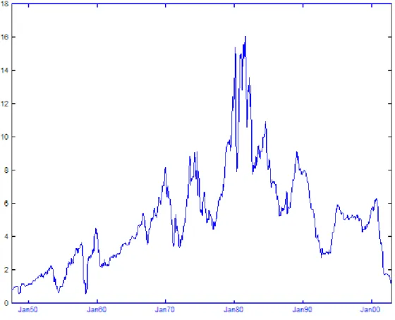
We analyze monthly data on the nominal three month US T-bill rate from July 1947 through December 2002. Prior to the beginning of this sample interest rates were …xed for a lengthy period so our data set is the longest available post-war sample with variable interest rates. The data source is the Center for Research in Security Prices at the Graduate School of Business, University of Chicago. T-bill yields are computed from the average of bid and ask prices and are continuously compounded 365 day rates. Figure 1 plots the monthly yields. We divide the data into two parts. Observations from the beginning of the sample through December 1997 are used as the estimation sample, while data from January 1998 through December 2002 (60 observations) are used as the forecasting (out-of-sample) period.
4.2
Prior Elicitation and Posterior Inference
In Section 2 we speci…ed a beta distribution for the diagonal elements of the transition probability matrix, a Normal-Wishart distribution for the meta-distribution parameters of the regression coe¢ cients and a Gamma-Exponential for the error term precision parameters. Implementation of our method requires assigning values to the associated hyperparameters. For the
pii’s we assume a non-informative prior for all the diagonal elements of (1),
i.e., a =b = 0:5. For the Normal-Wishart distribution, we specify = 0,
= 1000 Ir+1, v = 2 and V = Ir+1, where 0 is an (r+ 1 1) vector
of zeros, while Ir+1 is the (r+ 1 r+ 1) identity matrix. These values
re-‡ect no speci…c prior knowledge and are di¤use over sensible ranges of values for both the Normal and Wishart distribution. Similarly, we set 0 = 0:01,
c0 = 1 and d0 = 0:01, allowing the prior for v0 and d0 to be uninformative
over the positive real line.
We also conducted a prior sensitivity analysis to ensure that the empiri-cal results are robust to di¤erent prior beliefs. For the transition probability matrix, P; we modi…ed a and b to account for a wide set of regime dura-tions; we also changed the beta prior mean hyperparameters and , and the regime error term precision hyperparameters c0, d0 and 0. In all
cases we found the HMC estimates were insensitive to changes in the prior hyperparameters. More care is needed when dealing with the beta prior pre-cision hyperparameter V . For small values of its diagonal elements (less than 0:5), the meta distribution for the regression coe¢ cients will not allow enough variation across regimes, and as a consequence the regime regression coe¢ cients are clustered around the mean of the meta-distribution, b0.
Em-pirical results were found to be robust for values of the diagonal elements of
V greater than or equal to 1.
4.3
Model Estimates
In view of their empirical success and extensive use in forecasting13 we model the process underlying T-bill rates fytg as anrth order autoregressive (AR) 13See Pesaran and Timmermann (2004) for further references to the literature on
model allowing for up to K breaks over the observed sample fy1; :::::; yTg:14 yt= 8 > > > < > > > : 1;0+ 1;1yt 1+:::+ 1;ryt r+ 1 t; t = 1; :::; 1 2;0+ 2;1yt 1+:::+ 2;ryt r+ 2 t; t = 1+ 1; :::; 2 .. . K+1;0 + K+1;1yt 1+:::+ K+1;ryt r+ K+1 t; t= K + 1; :::; T: (19) Within the class of AR processes, this speci…cation is quite general and allows for intercept and slope shifts as well as changes in the error variances. Each regimej ,j = 1; :::K+1, is characterized by a vector of regression coe¢ cients,
j = j;0; j;1; ::: j;r
0
, and an error term variance, 2
j, fort= j 1+1; :::; j:
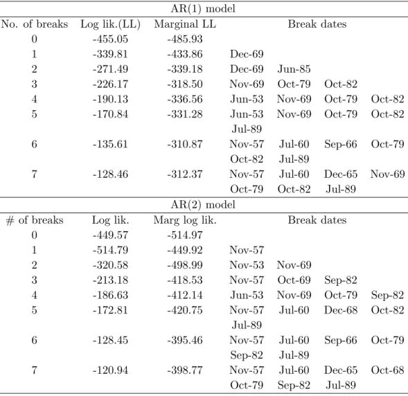
Following previous studies we consider …rst and second order autoregres-sive speci…cations for the T-bill rate. The AR(1) model is our base spec-i…cation and results for the AR(2) model are included to demonstrate the robustness of our empirical …ndings. For each AR speci…cation we obtain a di¤erent model by varying the number of breaks, K, and we rank these mod-els by means of their marginal likelihoods computed using the Chib method from Section 2.1. Table 1 reports maximized log-likelihood values, marginal log-likelihoods and break dates for values of K ranging from zero to seven. For both autoregressive speci…cations, the marginal log-likelihood is maxi-mized at K = 6. The models with K = 7 break points obtain basically the same marginal log-likelihood, suggesting that the additional break is not supported by the data.
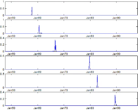
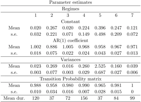
Figure 2 plots the posterior probability for the six break points under the AR(1) model. Results are nearly identical for the AR(2) model. The local unimodality of the posterior distributions shows that the break points are generally precisely estimated.15 For the autoregressive models with six break points, Tables 2, 3, 4 and 5 report the autoregressive parameters, variance, transition probability and the average number of months spent in each regime. In all regimes the interest rate is highly persistent and close to a unit root process. The error term variance is particularly high for regime 5 (lasting from October 1982 to July 1989), and quite low for regimes 1 (Sep 14Although structural break tests often do not reveal the form of the instability, a widely
used class of models assumes that it can be well approximated by a sequence of discrete structural breaks.
15In contrast, the plot for the model with seven break points (not shown here) had
a very wide posterior density for the 1969 break, providing further evidence against the inclusion of an additional break point.
1947 - Nov 1957), 3 (Jul 1960 - Sep 1966) and 7 (July 1989 - Dec 1997). Tables 3 and 5 report prior parameter estimates, i.e. the meta distribution parameters under the AR(1) and AR(2) models. For example, in the case of the AR(1) speci…cation, the two meta distributions are
j N 0:1908 0:9438 ; 0:2731 0:0088 0:1981 ; 2 j Gamma(0:7748;0:0431):
>From the properties of the Gamma distribution, the mean of the precision of the meta distribution is almost 18 and the standard error is around 20. These values are consistent with the values of the inverse of the variance estimates in Table 2.
4.4
Unit Root Dynamics
The persistent dynamics observed in some of the regimes may be a cause for concern when calculating multi-step forecasts. Unit roots or even explosive roots could a¤ect the meta distribution which averages parameter values across the regimes. To deal with this problem, we propose the following alternative constrained parameterization of the AR(1) model:
yt+1 = j j jyt+ t+1; j = 1; :::; K + 1; (20)
where t+1 N(0; 2j). If j = 0, the process has a unit root while if
0 < j < 2, it is a stationary AR(1) model. Notably, in the case with a unit root there is no drift irrespective of the value of j. Assuming that the
process is stationary, its long run mean is simply j.
We estimate our hierarchical HMC model under this new parameteriza-tion. To avoid explosive roots and negative unconditional mean, we constrain
j to lie in [0;1] and j to be strictly positive. We accomplish this by
as-suming that the priors for the regime regression parameters and error term precisions are
j N(b0;B0)I j 2A ; (21)
with j = j; j
0
, while the priors for the meta-distribution hyperparame-ters in this case become
b0 N ; I(b0 2A) (22)
B01 W v ;V 1 :
I(x2A) in (21) and (22) is an indicator function that equals 1 ifx belongs to A and is zero otherwise. A is the set [0;1) (0;1]. No changes are needed in the priors for the meta-distribution hyperparameters of the error term precision, v0 and d0. We obtain the same posterior densities as under
the unrestricted model although these distributions are now truncated due to the inequality constraints.
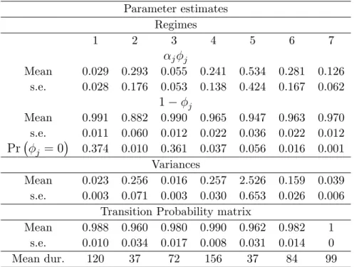
Tables 6 and 7 report estimates assuming six breaks. The detected break points are the same as those found for the unrestricted AR(1) model. To be comparable to the earlier tables, the regime coe¢ cients and meta distribution results refer to j j and 1 j. For each regime and for the meta
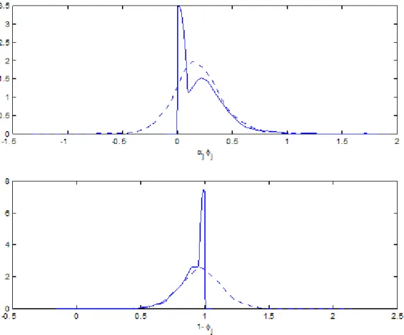
distribu-tion, Table 6 shows the probability of a unit root, calculated as Pr j = 0 . Regimes 1 and 3 are more likely to be non-stationary, both have a unit root probability slightly higher than one third. This is also re‡ected in the meta distribution results, Pr (b0(2) = 1) = 0:38. Figure 3 shows the posterior
den-sities for the meta distribution parameters for the unrestricted and restricted models.
4.5
Forecasts
We …nally turn to the calculation of out-of-sample predictive distributions. We base our results on the model with six breaks occurring over the es-timation sample, but later also present results based on Bayesian Model Averaging across di¤erent numbers of breaks using (17) and (18). Attention is restricted to the AR(1) speci…cation, since predictive distributions under the AR(2) model are very similar. We start from the end of the in-sample period T (December 1997) and compute predictive distributions for period
T +h (h = 1; ::;60) under the scenarios described in section 3. To obtain the predictive density under the no break scenario we use the information from the last regime of the hierarchical HMC model. To gain intuition we also show results under the meta distribution scenario which represents the opposite extreme case and assumes that a single break occurs at the begin-ning of the out-of-sample period, T + 1. This case draws a new vector of
regression parameters and a new error term variance from the meta distrib-ution. Finally, the hierarchical HMC forecast that allows for out-of-sample breaks is based on the scenarios in (16). We refer to this as the ‘composite’ forecast. This forecast assumes uninformative priors for both a and b, with
a0 = 1and b0 = 0:1. Di¤erent values fora0 and b0 were tried and the results
were found to be robust to changes in a0; b0.16
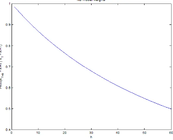
Figure 4 shows the weights on the ‘no break’model as a function of the forecast horizon. One minus this quantity is the weight assigned to draws from the meta distribution. As expected, the weight decreases monotonically in the forecast horizon, h, implying that higher weight is given to parameters drawn from the meta distribution the longer the forecast horizon and the higher therefore the chance of experiencing a break prior to T +h:
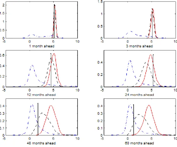
Figure 5 plots the associated forecast densities. The forecast horizon ranges from one to sixty months. As expected from the variance estimates in Table 2, under no break the predictive density is concentrated around its mean, while there is much more uncertainty under the meta distribution which balances di¤erences in parameter estimates across the seven break seg-ments. We also inspect graphically the performance of these forecasts. In each panel the actual (realized) value of the T-bill rate for that period is indicated by a vertical line. After year 2000, the Treasury bill rate declines signi…cantly. In fact, a separate Hidden Markov Chain run restricted only to the period 1998:01-2002:12 con…rmed that a break may have occurred at this time. Consequently, after this period the forecasts from the no break model are very poor while the composite model forecasts perform considerably bet-ter. The last three panels in Figure 5 show that the no break forecasts are upward biased and unable to capture the decline in the T-Bill rate while the composite forecasts are more accurate.
4.6
Forecast Evaluation
We next investigate the performance of the no break and hierarchical HMC models using the posterior predictive p-value approach. If the model …ts the data reasonably well, realized values of the T-bill rate in the out-of-sample period should not be too far out in the tails of the predictive density. To see 16The posterior means of the hyperparameters a and b are 28.54 and 0.83 while the
standard deviations are 17.26 and 0.44. The prior for the transition probabilities is, at the posterior mean ofa andb, a beta distribution with a mean of 0.9717 and a variance of 0.0311.
if this holds, for each of the models, M, we compute the percentile of the realized value, RyT+h
1 p(zj YT; M)dz and report how many times the model yields posterior predictivep-values below 0.05 or above 0.95, viewing an over-representation of such occurrences as evidence against a model.
Table 8 reports empirical results both for the full out-of-sample period, 1998:01-2002:12 and for the subperiod 2001:01-2002:12. We consider these samples separately due to the evidence of a break around the end of 2000. Forecasting performance is computed as averages across di¤erent horizons,h, based on forecasts originating from periodT (i.e. based onYT). In both cases
the forecast density based on the composite model outperforms forecasts from the model that assumes no new breaks. Results are particularly striking for the second subsample where the no break density leads to poor predictions two thirds of the time, while the composite model is never rejected.
We also computed root mean squared forecast errors under the no break and composite models - using both the restricted and unrestricted versions - based either on the posterior mean or the posterior mode of the density forecast as our point forecast of the future T-bill rate. This is a popular measure of forecasting performance. Table 9 shows that the composite model produces more precise point forecasts than the no break model, both in the restricted and unrestricted case. The constrained model seems to marginally outperform the unconstrained one.
When compared to the performance of forecasts from classical approaches, the root mean squared forecast error value of 1.36% from the composite model is substantially below the value generated by forecasts based on esti-mates from the full sample (2.06%), a …ve-year rolling window (2.00%) and discounted least squares (2.04%), assuming a discount factor of 0.95.
One last issue that may be relevant when forecasting T-Bill rates is the possible presence of autoregressive conditional heteroskedasticity (ARCH) in the residuals. To some extent our approach deals with this by letting the innovation variance vary across regimes so that the volatility parameter e¤ectively follows a step function. To investigate if the normalized residuals (scaled by the estimated standard deviation) still are heteroskedastic, we ran Lagrange Multiplier (LM) tests, regressing the squared normalized residuals on their lagged values. Even though some ARCH e¤ects remain in the scaled residuals, after scaling the residuals we found that theR2of the LM regression was reduced from 16% to 2%.
4.7
Uncertainty about the Number of in-sample Breaks
The empirical results presented thus far were computed from the hierarchical HMC model under the assumption of six breaks in the in-sample period. One can, however, argue that it is not reasonable to condition on the number of breaks. We therefore explicitly consider models with di¤erent numbers of break points, integrating out uncertainty about the number of break points in the data by means of the Bayesian model averaging formulas (17)-(18). Speci…cally, we consider between one and seven breaks in the data and assign equal prior probabilities to each of these models.Table 10 shows the posterior mass assigned to each of the models. A probability mass close to zero is assigned to the models with …ve or fewer break points while 82 and 18 percent of the posterior mass is assigned to the models with six and seven break points, respectively.
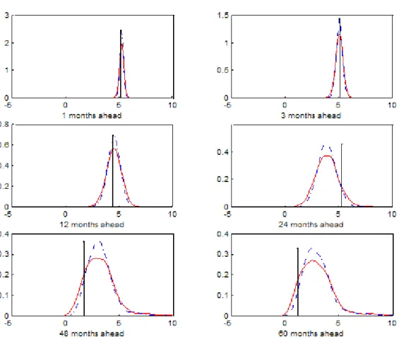
Figure 6 plots the combined predictive density under Bayesian model averaging along with the predictive density that conditions on six breaks. The graphs reveal that the two densities are very similar. It is therefore not surprising that the out-of-sample root mean squared forecast error values obtained under the two approaches are basically the same and di¤er only after the fourth decimal. This means that the forecasting results reported so far are very robust to uncertainty about the number of in-sample breaks.
5
Conclusion
The key contribution of this paper has been to introduce a hierarchical hidden Markov chain approach to model the meta distribution for the parameters of the stochastic process underlying structural breaks. This allowed us to forecast economic time series that are subject to structural breaks. Our approach is quite general and can be implemented in di¤erent ways from that assumed in the current paper. For example, the state transitions could be allowed to depend on time-varying regressors tracking factors related to uncertainty about institutional shifts or the likelihood of macroeconomic or oil price shocks. When applied to autoregressive speci…cations for U.S. T-Bill rates, an out-of-sample forecasting exercise found that our approach produces better forecasts than methods that ignore the possibility of future breaks.
The simple ‘no new break’approach that forecasts using parameter esti-mates solely from the last post-break period can be expected to perform well
when the number of observations from the last regime is su¢ ciently large to deliver precise parameter estimates, and the possibility of new breaks occur-ring over the forecast horizon is very small, c.f. Pesaran and Timmermann (2004). However, when forecasting many periods ahead or when breaks occur relatively frequently so the last break point is close to the end of the sample and a new break is likely to occur shortly after the end of the estimation sample this approach is unlikely to produce satisfactory forecasts.
Intuition for why our approach appears to work quite well in forecasting interest rates is that it e¤ectively shrinks the new parameters drawn after a break towards the meta distribution. Shrinkage has widely been found to be a useful device for improving forecasting performance in the presence of parameter estimation and model uncertainty, c.f. Diebold and Pauly (1990), Stock and Watson (2003), Garratt, Lee, Pesaran and Shin (2003), and Aiol… and Timmermann (2004). Here it appears to work because the number of breaks that can be identi…ed empirically tends to be small and the parameters of the meta distribution from which such breaks are drawn is reasonably precisely estimated.
References
[1] Aiol…, M. and A. Timmermann, 2004, Persistence in Forecasting Performance and Conditional Combination Strategies, Unpublished Manuscript, UCSD. [2] Alogoskou…s, G.S. and R. Smith, 1991, The Phillips Curve, the Persistence
of In‡ation, and the Lucas Critique: Evidence from Exchange Rate Regimes. American Economic Review 81, 1254-1275.
[3] Ang, A., and G., Bekaert, 2002, Regime Switches in Interest Rates, Journal of Business and Economic Statistics, 20, 163-182.
[4] Bai, J. and P. Perron, 1998, Estimating and Testing Linear Models with Multiple Structural Changes. Econometrica 66, 47-78.
[5] Bai, J. and P. Perron, 2003, Computation and Analysis of Multiple Structural Change Models, Journal of Applied Econometrics, 18, 1-22.
[6] Carlin, B., A.E. Gelfand and A.F.M. Smith, 1992, Hierarchical Bayesian analysis of changepoint problems, Applied Statistics, 41, 389-405.
[7] Chib, S., 1995, Marginal Likelihood from the Gibbs output, Journal of the American Statistical Association, 90, 1313-1321.
[8] Chib, S., 1996, Calculating Posterior Distribution and Modal Estimates in Markov Mixture Models, Journal of Econometrics, 75, 79-97.
[9] Chib, S., 1998, Estimation and Comparison of Multiple Change Point Models, Journal of Econometrics, 86, 221-241.
[10] Chib, S. and I. Jeliazkov, 2001, Marginal Likelihood from the Metropolis-Hastings Output, Journal of the American Statistical Association, 96, 270-281.
[11] Clements, M.P. and D.F. Hendry, 1998, Forecasting Economic Time Series, Cambridge University Press.
[12] Clements, M.P. and D.F. Hendry, 1999, Forecasting Non-stationary Economic Time Series, The MIT Press.
[13] Diebold, F.X and P. Pauly, 1990, The Use of Prior Information in Forecast Combination, International Journal of Forecasting, 6, 503-508.
[14] Garratt, A, K. Lee, M. H. Pesaran and Y. Shin, 2003, Forecast Uncertainties in Macroeconometric Modelling: An Application to the UK Economy. Journal of the American Statistical Association, 98, 829-838.
[15] Garcia, R. and P. Perron, 1996, An Analysis of the Real Interest Rate under Regime Shifts. Review of Economics and Statistics, 78, 111-125.
[16] Gelman, A., Carlin, J.B., Stern, H.S. and Rubin, D., 2002, Bayesian Data Analysis, Second Edition, Chapman & Hall Editors.
[17] George, E. I., U. E. Makov and A. F. M. Smith, 1993, Conjugate Likelihood Distributions, Scandinavian Journal of Statistics, 20, 147-156.
[18] Gray, S., 1996, “Modeling the Conditional Distribution of Interest Rates as Regime-Switching Process”, Journal of Financial Economics, 42, 27-62. [19] Hamilton, J.D., 1988, Rational Expectations Econometric Analysis of
Changes in Regime. An Investigation of the Term Structure of Interest Rates. Journal of Economic Dynamics and Control, 12, 385-423.
[20] Inclan, C., 1994, Detection of Multiple Changes of Variance Using Posterior Odds. Journal of Business and Economic Statistics, 11, 289-300.
[21] Je¤reys, H., 1961, Theory of Probability, Oxford University Press, Oxford. [22] Kim, C.J., C.R. Nelson and J. Piger, 2004, The Less-Volatile US Economy.
A Bayesian Investigation of Timing, Breadth, and Potential Explanations. Journal of Business and Economic Statistics 22, 80-93.
[23] Koop, G., 2003, Bayesian Econometrics, John Wiley & Sons, New York. [24] Koop, G. and S. Potter, 2001, Are Apparent Findings of Nonlinearity Due
to Structural Instability in Economic Time Series? Econometrics Journal, 4, 37-55.
[25] Maheu, J.M. and S. Gordon, 2004, Learning, Forecasting and Structural Breaks. Manuscript University of Toronto.
[26] McCulloch, R.E. and R. Tsay, 1993, Bayesian Inference and Prediction for Mean and Variance Shifts in Autoregressive Time Series. Journal of the Amer-ican Statistical Association 88, 965-978.
[27] Pastor, L. and R.F. Stambaugh, 2001, The Equity Premium and Structural Breaks. Journal of Finance, 56, 1207-1239.
[28] Pesaran, M.H. and A. Timmermann, 2002, Market Timing and Return Pre-diction under Model Instability. Journal of Empirical Finance, 9, 495-510. [29] Pesaran, M.H. and A. Timmermann, 2004, Small Sample Properties of
Fore-casts from Autoregressive Models under Structural Breaks. Forthcoming in Journal of Econometrics.
[30] Siliverstovs, B. and D. van Dijk, 2002, Forecasting Industrial Production with Linear, Non-linear and Structural Breaks Models. Manuscript DIW Berlin. [31] Stock, J.H. and M.W. Watson, 1996, Evidence on Structural Instability in
Macroeconomic Time Series Relations, Journal of Business and Economic Statistics, 14, 11-30.
[32] Stock, J.H. and M. Watson, 2003, Combination Forecasts of Output Growth in a Seven-Country Data Set. Forthcoming, Journal of Forecasting.
Appendix A. Gibbs Sampler for the Multiple Regime
Model
The posterior distribution of interest is ( ;p;STj YT), where
= 1; 21; :::; K+1; 2K+1;b0;B0; v0; d0
includes the K + 1 regime coe¢ cients and the prior locations and scales, ST = (s1; :::; sT) is the collection of values of the latent state variable, YT = (y1; :::; yT)0; and p= (p11; p22;:::; pKK)0 summarizes the unknown
pa-rameters of the transition probability matrix in (1). The Gibbs sampler applied to our set up works as follows: First the states are simulated condi-tional on the data, YT;and the parameters and, second, the parameters are
simulated conditional on the data and ST. Speci…cally, the Gibbs sampling
is implemented by simulating the following set of conditional distributions: 1. (STj ;p;YT)
2. ( ;j YT;p;ST)
3. (pj ST)
where we have used the identity ( ;pj ST;YT) = ( j YT;p;ST) (pj ST),
noting that under our assumptions (pj ;ST;YT) = (pj ST).
The simulation of the states ST requires ‘forward’and ‘backward’passes
through the data. De…ne St = (s1; :::; st) and St+1 = (st+1; :::; sT) as the
state history up to time t and from time t to T, respectively. We partition the states’joint density as follows:
p(sT 1j YT; sT; ;p) p(stj YT;St+1; ;p) p(s1j YT;S2; ;p):
(A1) Chib (1995) shows that the generic element of (A1) can be decomposed as
p(stj YT;St+1; ;p)/p(stj YT; ;p)p(stjst 1; ;p); (A2)
where the normalizing constant is easily obtained sincesttakes only two
val-ues conditional on the value taken byst+1. The second term in (A2) is simply
the transition probability from the Markov chain. The …rst term can be com-puted by a recursive calculation (the forward pass through the data) where,
for givenp(st 1j Yt 1; ;p), we obtainp(stj Yt; ;p)and p(st+1j Yt+1; ;p),
..., p(sTj Yt; ;p). Supposep(st 1j Yt 1; ;p) is available, then p(st =kj Yt; ;p) = p(st =kj Yt 1; ;p) f(ytj Yt 1; k) k X l=k 1 p(st=lj Yt 1; ;p) f(ytj Yt 1; l) ; where, for k= 1;2; :::; K + 1; p(st=kj Yt 1; ;p) = k X l=k 1 plk p(st 1 =lj Yt 1; ;p);
and plk is the Markov transition probability.
For a given set of simulated states,ST, the data is partitioned into K+ 1
groups. To obtain the conditional distributions for the regression parameters, prior locations and scales, note that the conditional distribution of the j’s
are mutually independent with
j 2j;b0;B0; v0; d0;p;ST;YT N j; Vj ;
where
Vj = 2X0jXj +B01 1
; j =Vj 2X0jyj+B01b0 ;
Xj is the matrix of observations on the regressors in regime j, and yj is the
vector of observations on the dependent variable in regime j:
De…ning 1:k+1 = 01; :::; 0K+1 0 and 2 1:k+1 = 21; :::; 2K+1 0 , the densi-ties of the location and scale parameters of the regression parameter meta-distribution, b0 and B0, can be written
b0j 1:k+1; 2 1:k+1;B0; v0; d0;p;ST;YT N ; B01 1:k+1; 21:k+1;b0; v0; d0;p;ST;YT W v ;V 1 ; where = 1+ (K+ 1)B01 1 = B01 J P j=1 j + 1 ! ;
and v = v + (K+ 1) V = J P j=1 j b0 j b0 0+V :
Moving to the posterior for the precision parameters within each regime, note that 2 j j;b0;B0; v0; d0;p;ST;YT G 0 B B B @ v0+ j P i= j 1+1 (yi Xi i)0(yi Xi i) 2 ; d0+nj 2 1 C C C A;
where nj is the number of observations assigned to regime j. The location
and scale parameters for the error term precision are then updated as follows:
v0j 1:k+1; 1:2k+1;b0;B0; d0;p;ST;YT / KY+1 j=1 G j2 v0; d0 Exp v0j 0 (A3) d0j 1:k+1; 2 1:k+1;b0;B0; v0;p;ST;YT G v0(K + 1) +c0; KX+1 j=1 2 j +d0 !
Drawingv0 from (A2) is slightly more complicated since we cannot make
use of any standard distributions. We therefore introduce a Metropolis-Hastings (M-H) step in the Gibbs sampling algorithm. At each loop of the Gibbs sampling we draw a value v0 from a Gamma distributed candidate generating density of the form
q v0jvg0 1 G &; &=vg0 1 :
This candidate generating density is centered on the last accepted value of v0 in the chain, v0g 1, while the parameter & de…nes the variance of the
density and, as a by-product, the rejection in the M-H step. Higher values of & mean a smaller variance for the candidate generating density and thus
a smaller rejection rate. The acceptance probability is given by v0jv0g 1 = min " (v0j ; 2;b 0;B0; d0;p;ST;YT)=q v0jv g 1 0 v0g 1 ; 2;b 0;B0; d0;p;ST;YT =q v0g 1 v0 ;1 # : (A4) With probability v0jv0g 1 the candidate value v0 is accepted as the next value in the chain, while with probability 1 v0jv0g 1 the chain remains at vg0 1. The acceptance ratio penalizes and rejects values of v0
drawn from low posterior density areas.
Finally, p is easily simulated from (pj ST) since, under the beta prior
in (2) and given the simulated states, ST, the posterior distribution of pii is
Beta(a+nii; b+ 1)whereniiis the number of one step transitions from state
i to state iin the sequence Sn.
Appendix B. Estimation of Break Point Model
This appendix provides details of how we implement the Chib (1995) method for comparing models with di¤erent numbers of break points and how we compute the di¤erent components of (8).
Consider the points ( ;p ) in ( ;p), which could be maximum likeli-hood estimates or posterior means or modes. The likelilikeli-hood function eval-uated at and p is available from the proposed parameterization of the change point model and can be obtained as
logf(YTj ;p ) = T
X
t=1
logf(ytj Yt 1; ;p );
where the one-step-ahead predictive density is
f(ytj Yt 1; ;p ) =
KX+1
k=1
f(ytj Yt 1; ;p ; st =k)p(st=kj Yt 1; ;p ):
For simplicity we suppressed the model indicator. The prior density evaluated at the posterior means or modes is easily computed since it is known in advance. The denominator of (8) needs some explanation, however. We can decompose the posterior density as
where ( j YT) = Z ( j YT;ST)p(STj YT)dST; and (p j ;YT) = Z (p j ST) (STj ;YT)dST:
The …rst part can be estimated as b( j YT) = G 1 G
P
g=1
( j YT;ST;g)
using G draws from the run of the Markov Chain Monte Carlo algorithm. The second part (p j ;YT)requires an additional simulation of the Gibbs
sampler for [ST;g] G
g=1 from (STj ;YT). These draws are obtained by
adding steps at the end of the original Gibbs sampling in order to simulate ST conditional on (YT; ;p ) and p conditional on (YT; ;ST).
The idea outlined above is easily extended to the case where the Gibbs sampler divides into B blocks, i.e. = ( 1; 2; :::; B). Since
( j YT) = ( 1j YT) ( 2j 1;YT) Bj 1; :::; B 1;YT ;
we can use di¤erent Gibbs sampling steps to calculate the posterior ( j Y). In our example we have 1 = j, 2 = j2 (j = 1; :::; K + 1), 3 = b0, 4 =B0, 5 =v0 and 6 =d0. The Chib method can become
computation-ally demanding, but the various sampling steps all have the same structure. For some of the blocks in the hierarchical Hidden Markov Chain model, the full conditional densities are non-standard, and sampling requires the use of the Metropolis-Hastings algorithm (see for example the precision prior hyper-parameter v0). The original Chib 1995 algorithm is then modi…ed following
Figure 2: Posterior probability of break occurrence for the AR(1) model, assumingK= 6
Figure 3: Posterior density of the meta distribution parameters b0 under the
Figure 4: Posterior probability of staying in regime K + 1 at time T + h,
Figure 5: Predictive densities under three models for the T-Bill series. The graphs show the predictive distributions for the T-Bill series under various forecast horizons. The dotted line represents the forecast assuming no break point in the new data by using only the information from the last regime (assumingK=6), the solid line represents the ’meta-distribution’forecast under the assumption of a new break occuring immediately after the end of the estimation sample, while the dash-dotted line is the predictive density from the composite model.
Figure 6: Composite predictive densities under Bayesian model averaging (dashed dotted line) and under the model with six breaks (solid line).
AR(1) model
No. of breaks Log lik.(LL) Marginal LL Break dates 0 -455.05 -485.93
1 -339.81 -433.86 Dec-69
2 -271.49 -339.18 Dec-69 Jun-85
3 -226.17 -318.50 Nov-69 Oct-79 Oct-82
4 -190.13 -336.56 Jun-53 Nov-69 Oct-79 Oct-82 5 -170.84 -331.28 Jun-53 Nov-69 Oct-79 Oct-82
Jul-89
6 -135.61 -310.87 Nov-57 Jul-60 Sep-66 Oct-79 Oct-82 Jul-89
7 -128.46 -312.37 Nov-57 Jul-60 Dec-65 Nov-69 Oct-79 Oct-82 Jul-89
AR(2) model
# of breaks Log lik. Marg log lik. Break dates 0 -449.57 -514.97
1 -514.79 -449.92 Nov-57
2 -320.58 -498.99 Nov-53 Nov-69
3 -213.18 -418.53 Nov-57 Oct-69 Sep-82
4 -186.63 -412.14 Jun-53 Nov-69 Oct-79 Sep-82 5 -172.81 -420.75 Nov-57 Jul-60 Dec-68 Oct-82
Jul-89
6 -128.45 -395.46 Nov-57 Jul-60 Sep-66 Oct-79 Sep-82 Jul-89
7 -120.94 -398.77 Nov-57 Jul-60 Dec-65 Oct-68 Oct-79 Sep-82 Jul-89
Table 1: Model comparison. This table shows the log likelihood and the marginal log likelihood estimates for di¤erent numbers of breaks along with the time of the break points for the di¤erent models. The top and bottom panels display results for the AR(1) and AR(2) models, respectively.
Parameter estimates Regimes 1 2 3 4 5 6 7 Constant Mean 0.020 0.267 0.020 0.224 0.396 0.247 0.121 s.e. 0.032 0.221 0.071 0.149 0.498 0.209 0.072
AR(1) coe¢ cient
Mean 1.002 0.886 1.005 0.968 0.958 0.967 0.971 s.e. 0.018 0.075 0.022 0.024 0.043 0.027 0.013
Variances
Mean 0.023 0.269 0.016 0.260 2.525 0.160 0.039 s.e. 0.003 0.077 0.003 0.029 0.687 0.027 0.006
Transition Probability matrix
Mean 0.988 0.958 0.980 0.990 0.965 0.981 1 s.e. 0.010 0.034 0.016 0.007 0.028 0.015 0 Mean dur. 120 37 72 156 37 84 99
Table 2: Posterior parameter estimates for the unconstrained AR(1) hierarchical Hidden Markov Chain model with six break points.
Mean Parameters
Mean s.e. 95% conf interval
b0(1) 0.191 0.211 -0.209 0.633 b0(2) 0.944 0.161 0.619 1.220 Variance Parameters Mean s.e. B0(1;1) 0.273 0.312 B0(2;2) 0.198 0.147
Error term precision
Mean s.e. 95% conf interval
v0 0.775 0.344 0.260 1.500 d0 0.043 0.024 0.010 0.101
Table 3: Prior parameter estimates for the unconstrained AR(1) hierarchical Hidden Markov Chain model with six break points.
Parameter estimates Regimes 1 2 3 4 5 6 7 Constant Mean 0.023 0.300 0.009 0.208 0.572 0.290 0.108 s.e. 0.034 0.225 0.069 0.156 0.593 0.212 0.069
AR(1) coe¢ cient
Mean 1.044 1.040 0.950 0.934 1.153 1.098 1.267 s.e. 0.091 0.161 0.112 0.080 0.153 0.108 0.092
AR(2) coe¢ cient
Mean -0.045 -0.162 0.059 0.036 -0.208 -0.136 -0.292 s.e. 0.093 0.160 0.115 0.081 0.156 0.109 0.090
Variances
Mean 0.023 0.2591 0.015 0.260 2.468 0.160 0.035 s.e. 0.003 0.071 0.003 0.031 0.646 0.027 0.005
Transition Probability matrix
Mean 0.988 0.959 0.980 0.990 0.961 0.982 1 s.e. 0.010 0.033 0.016 0.008 0.031 0.014 0
Table 4: Posterior parameter estimates for the unconstrained AR(2) hierarchical Hidden Markov Chain model with six break points.
Mean Parameters
Mean s.e. 95% conf interval
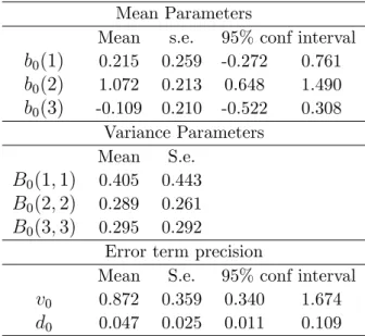
b0(1) 0.215 0.259 -0.272 0.761 b0(2) 1.072 0.213 0.648 1.490 b0(3) -0.109 0.210 -0.522 0.308 Variance Parameters Mean S.e. B0(1;1) 0.405 0.443 B0(2;2) 0.289 0.261 B0(3;3) 0.295 0.292
Error term precision
Mean S.e. 95% conf interval
v0 0.872 0.359 0.340 1.674 d0 0.047 0.025 0.011 0.109
Table 5: Prior parameter estimates for the unconstrained AR(2) hierarchical Hidden Markov Chain model with six break points.
Parameter estimates Regimes 1 2 3 4 5 6 7 j j Mean 0.029 0.293 0.055 0.241 0.534 0.281 0.126 s.e. 0.028 0.176 0.053 0.138 0.424 0.167 0.062 1 j Mean 0.991 0.882 0.990 0.965 0.947 0.963 0.970 s.e. 0.011 0.060 0.012 0.022 0.036 0.022 0.012 Pr j = 0 0.374 0.010 0.361 0.037 0.056 0.016 0.001 Variances Mean 0.023 0.256 0.016 0.257 2.526 0.159 0.039 s.e. 0.003 0.071 0.003 0.030 0.653 0.026 0.006
Transition Probability matrix
Mean 0.988 0.960 0.980 0.990 0.962 0.982 1 s.e. 0.010 0.034 0.017 0.008 0.031 0.014 0 Mean dur. 120 37 72 156 37 84 99
Table 6: Posterior parameter estimates for the AR(1) hierarchical Hidden Markov Chain model with six break points under the constrained parameterization in (19).
Mean Parameters
Mean s.e. 95% conf interval
b0(1) 0.173 0.198 0 0.650 b0(2) 0.914 0.112 0.627 1 Pr (b0(2) = 1) 0.383 Variance Parameters Mean s.e. B0(1;1) 0.282 0.254 B0(2;2) 0.189 0.140
Error term precision
Mean s.e. 95% conf interval
v0 0.858 0.359 0.335 1.677 d0 0.047 0.026 0.012 0.114
Table 7: Prior parameter estimates for the AR(1) hierarchical Hidden Markov Chain model with six break points under the constrained parameterization in (19).
Violations %
1998:01-2002:12 2001:01-2002:12 No break 0.350 0.667 Combined 0.183 0
Table 8: Percentage of times the posterior predictive p-value lies outside the 0.05-0.95 interval under the model assuming no new break points after the end of the sample and the composite hierarchical Hidden Markov chain model.
Unconstrained Constrained Posterior Mean No break 1.575 1.579 Combined 1.366 1.363 Posterior Mode No break 1.607 1.594 Combined 1.288 1.294
Table 9: Root mean squared forecast error for the posterior means and modes of the predictive densities under the model assuming no new break points after the end of the sample and the constrained and unconstrained composite hierarchical Hidden Markov chain models.
# of breaks Posterior Prob
0 7.67E-77 1 3.15E-54 2 4.14E-13 3 3.97E-04 4 5.69E-12 5 1.12E-09 6 0.817 7 0.182
Table 10: Model Posterior Probabilities for di¤erent number of in sample break points. The posterior probabilities are computed by means of the margial log likelihood of table 1.
CESifo Working Paper Series
(for full list see www.cesifo.de)
___________________________________________________________________________ 1172 Bernd Huber and Marco Runkel, Tax Competition, Excludable Public Goods and User
Charges, April 2004
1173 John McMillan and Pablo Zoido, How to Subvert Democracy: Montesinos in Peru, April 2004
1174 Theo Eicher and Jong Woo Kang, Trade, Foreign Direct Investment or Acquisition: Optimal Entry Modes for Multinationals, April 2004
1175 Chang Woon Nam and Doina Maria Radulescu, Types of Tax Concessions for Attracting Foreign Direct Investment in Free Economic Zones, April 2004
1176 M. Hashem Pesaran and Andreas Pick, Econometric Issues in the Analysis of Contagion, April 2004
1177 Steinar Holden and Fredrik Wulfsberg, Downward Nominal Wage Rigidity in Europe, April 2004
1178 Stefan Lachenmaier and Ludger Woessmann, Does Innovation Cause Exports? Evidence from Exogenous Innovation Impulses and Obstacles, April 2004
1179 Thiess Buettner and Johannes Rincke, Labor Market Effects of Economic Integration – The Impact of Re-Unification in German Border Regions, April 2004
1180 Marko Koethenbuerger, Leviathans, Federal Transfers, and the Cartelization Hypothesis, April 2004
1181 Michael Hoel, Tor Iversen, Tore Nilssen, and Jon Vislie, Genetic Testing and Repulsion from Chance, April 2004
1182 Paul De Grauwe and Gunther Schnabl, Exchange Rate Regimes and Macroeconomic Stability in Central and Eastern Europe, April 2004
1183 Arjan M. Lejour and Ruud A. de Mooij, Turkish Delight – Does Turkey’s accession to the EU bring economic benefits?, May 2004
1184 Anzelika Zaiceva, Implications of EU Accession for International Migration: An Assessment of Potential Migration Pressure, May 2004
1185 Udo Kreickemeier, Fair Wages and Human Capital Accumulation in a Global Economy, May 2004
1187 Pablo Arocena, Privatisation Policy in Spain: Stuck Between Liberalisation and the Protection of Nationals’ Interests, May 2004
1188 Günter Knieps, Privatisation of Network Industries in Germany: A Disaggregated Approach, May 2004
1189 Robert J. Gary-Bobo and Alain Trannoy, Efficient Tuition Fees, Examinations, and Subsidies, May 2004
1190 Saku Aura and Gregory D. Hess, What’s in a Name?, May 2004
1191 Sjur Didrik Flåm and Yuri Ermoliev, Investment Uncertainty, and Production Games, May 2004
1192 Yin-Wong Cheung and Jude Yuen, The Suitability of a Greater China Currency Union, May 2004
1193 Inés Macho-Stadler and David Pérez-Castrillo, Optimal Enforcement Policy and Firms’ Emissions and Compliance with Environmental Taxes, May 2004
1194 Paul De Grauwe and Marianna Grimaldi, Bubbles and Crashes in a Behavioural Finance Model, May 2004
1195 Michel Berne and Gérard Pogorel, Privatization Experiences in France, May 2004
1196 Andrea Galeotti and José Luis Moraga-González, A Model of Strategic Targeted Advertising, May 2004
1197 Hans Gersbach and Hans Haller, When Inefficiency Begets Efficiency, May 2004
1198 Saku Aura, Estate and Capital Gains Taxation: Efficiency and Political Economy Consideration, May 2004
1199 Sandra Waller and Jakob de Haan, Credibility and Transparency of Central Banks: New Results Based on Ifo’s World Economicy Survey, May 2004
1200 Henk C. Kranendonk, Jan Bonenkamp, and Johan P. Verbruggen, A Leading Indicator for the Dutch Economy – Methodological and Empirical Revision of the CPB System, May 2004
1201 Michael Ehrmann, Firm Size and Monetary Policy Transmission – Evidence from German Business Survey Data, May 2004
1202 Thomas A. Knetsch, Evaluating the German Inventory Cycle – Using Data from the Ifo Business Survey, May 2004
1203 Stefan Mittnik and Peter Zadrozny, Forecasting Quarterly German GDP at Monthly Intervals Using Monthly IFO Business Conditions Data, May 2004
1204 Elmer Sterken, The Role of the IFO Business Climate Indicator and Asset Prices in German Monetary Policy, May 2004
1205 Jan Jacobs and Jan-Egbert Sturm, Do Ifo Indicators Help Explain Revisions in German Industrial Production?, May 2004
1206 Ulrich Woitek, Real Wages and Business Cycle Asymmetries, May 2004
1207 Burkhard Heer and Alfred Maußner, Computation of Business Cycle Models: A Comparison of Numerical Methods, June 2004
1208 Costas Hadjiyiannis, Panos Hatzipanayotou, and Michael S. Michael, Pollution and Capital Tax Competition within a Regional Block, June 2004
1209 Stephan Klasen and Thorsten Nestmann, Population, Population Density, and Technological Change, June 2004
1210 Wolfgang Ochel, Welfare Time Limits in the United States – Experiences with a New Welfare-to-Work Approach, June 2004
1211 Luis H. R. Alvarez and Erkki Koskela, Taxation and Rotation Age under Stochastic Forest Stand Value, June 2004
1212 Bernard M. S. van Praag, The Connexion Between Old and New Approaches to Financial Satisfaction, June 2004
1213 Hendrik Hakenes and Martin Peitz, Selling Reputation When Going out of Business, June 2004
1214 Heikki Oksanen, Public Pensions in the National Accounts and Public Finance Targets, June 2004
1215 Ernst Fehr, Alexander Klein, and Klaus M. Schmidt, Contracts, Fairness, and Incentives, June 2004
1216 Amihai Glazer, Vesa Kanniainen, and Panu Poutvaara, Initial Luck, Status-Seeking and Snowballs Lead to Corporate Success and Failure, June 2004
1217 Bum J. Kim and Harris Schlesinger, Adverse Selection in an Insurance Market with Government-Guaranteed Subsistence Levels, June 2004
1218 Armin Falk, Charitable Giving as a Gift Exchange – Evidence from a Field Experiment, June 2004
1219 Rainer Niemann, Asymmetric Taxation and Cross-Border Investment Decisions, June 2004
1220 Christian Holzner, Volker Meier, and Martin Werding, Time Limits on Welfare Use under Involuntary Unemployment, June 2004
1221 Michiel Evers, Ruud A. de Mooij, and Herman R. J. Vollebergh, Tax Competition under Minimum Rates: The Case of European Diesel Excises, June 2004
1222 S. Brock Blomberg and Gregory D. Hess, How Much Does Violence Tax Trade?, June 2004
1223 Josse Delfgaauw and Robert Dur, Incentives and Workers’ Motivation in the Public Sector, June 2004
1224 Paul De Grauwe and Cláudia Costa Storti, The Effects of Monetary Policy: A Meta-Analysis, June 2004
1225 Volker Grossmann, How to Promote R&D-based Growth? Public Education Expenditure on Scientists and Engineers versus R&D Subsidies, June 2004
1226 Bart Cockx and Jean Ries, The Exhaustion of Unemployment Benefits in Belgium. Does it Enhance the Probability of Employment?, June 2004
1227 Bertil Holmlund, Sickness Absence and Search Unemployment, June 2004
1228 Klaas J. Beniers and Robert Dur, Politicians’ Motivation, Political Culture, and Electoral Competition, June 2004
1229 M. Hashem Pesaran, General Diagnostic Tests for Cross Section Dependence in Panels, July 2004
1230 Wladimir Raymond, Pierre Mohnen, Franz Palm, and Sybrand Schim van der Loeff, An Empirically-Based Taxonomy of Dutch Manufacturing: Innovation Policy Implications, July 2004
1231 Stefan Homburg, A New Approach to Optimal Commodity Taxation, July 2004
1232 Lorenzo Cappellari and Stephen P. Jenkins, Modelling Low Pay Transition Probabilities, Accounting for Panel Attrition, Non-Response, and Initial Conditions, July 2004
1233 Cheng Hsiao and M. Hashem Pesaran, Random Coefficient Panel Data Models, July 2004
1234 Frederick van der Ploeg, The Welfare State, Redistribution and the Economy, Reciprocal Altruism, Consumer Rivalry and Second Best, July 2004
1235 Thomas Fuchs and Ludger Woessmann, What Accounts for International Differences in Student Performance? A Re-Examination Using PISA Data, July 2004
1236 Pascalis Raimondos-Møller and Alan D. Woodland, Measuring Tax Efficiency: A Tax Optimality Index, July 2004
1237 M. Hashem Pesaran, Davide Pettenuzzo, and Allan Timmermann, Forecasting Time Series Subject to Multiple Structural Breaks, July 2004