Linking CGE and Microsimulation Models: A Comparison of Different Approaches

econ

stor

www.econstor.eu

Der Open-Access-Publikationsserver der ZBW – Leibniz-Informationszentrum Wirtschaft The Open Access Publication Server of the ZBW – Leibniz Information Centre for Economics

Nutzungsbedingungen:

Die ZBW räumt Ihnen als Nutzerin/Nutzer das unentgeltliche, räumlich unbeschränkte und zeitlich auf die Dauer des Schutzrechts beschränkte einfache Recht ein, das ausgewählte Werk im Rahmen der unter

→ http://www.econstor.eu/dspace/Nutzungsbedingungen nachzulesenden vollständigen Nutzungsbedingungen zu vervielfältigen, mit denen die Nutzerin/der Nutzer sich durch die erste Nutzung einverstanden erklärt.

Terms of use:

The ZBW grants you, the user, the non-exclusive right to use the selected work free of charge, territorially unrestricted and within the time limit of the term of the property rights according to the terms specified at

→ http://www.econstor.eu/dspace/Nutzungsbedingungen By the first use of the selected work the user agrees and declares to comply with these terms of use.

Colombo, Giulia

Working Paper

Linking CGE and Microsimulation

Models: A Comparison of Different

Approaches

ZEW Discussion Papers, No. 08-054

Provided in cooperation with:

Zentrum für Europäische Wirtschaftsforschung (ZEW)

Suggested citation: Colombo, Giulia (2008) : Linking CGE and Microsimulation Models: A Comparison of Different Approaches, ZEW Discussion Papers, No. 08-054, http:// hdl.handle.net/10419/24750

Dis cus si on Paper No. 08-054

Linking CGE and Microsimulation Models:

A Comparison of Different Approaches

Dis cus si on Paper No. 08-054

Linking CGE and Microsimulation Models:

A Comparison of Different Approaches

Giulia Colombo

Die Dis cus si on Pape rs die nen einer mög lichst schnel len Ver brei tung von neue ren For schungs arbei ten des ZEW. Die Bei trä ge lie gen in allei ni ger Ver ant wor tung

der Auto ren und stel len nicht not wen di ger wei se die Mei nung des ZEW dar.

Dis cus si on Papers are inten ded to make results of ZEW research prompt ly avai la ble to other eco no mists in order to encou ra ge dis cus si on and sug gesti ons for revi si ons. The aut hors are sole ly

respon si ble for the con tents which do not neces sa ri ly repre sent the opi ni on of the ZEW. Download this ZEW Discussion Paper from our ftp server:

Linking CGE and Microsimulation Models:

A Comparison of Different Approaches

Giulia Colombo

Juli 2008

Abstract

In the paper we describe in detail how to build linked CGE-microsimulation models (using fictitious data) following three main approaches: one in accordance with the fully integrated approach and the other two according to the layered approach – the so-called Top-Down and Top-Down/Bottom-Up ap-proaches. After this, we implement the same policy reform in each of the three models. Results show that all three approaches yield different results especially in terms of income distribution and poverty, although analysed within the same economy and under the same policy simulation. We then analyse in more detail the TD/BU approach as developed by Savard (2003) and, in order to avoid possible devia-tions due to data inconsistencies, we propose an alternative way of taking into account feedback effects from the micro level of analysis into the CGE model.

JEL classification: C68, C15, C35, D31

Keywords: CGE models, microsimulation, income distribution.

*

Centre for European Economic Research (ZEW)

Department of Labour Markets, Human Resources and Social Policy L7,1 Mannheim

Tel +49 621 1235 367 [email protected]

I would like to thank in particular Stefan Boeters and Nicole Gürtzgen for their precious comments. Thanks are also due to Marco Missaglia for his constant support.

Zusammenfassung

Die wirtschaftswissenschaftliche Literatur zu Ungleichheit und Armut verknüpft immer häufi-ger makroökonomische berechenbare allgemeine Gleichgewichtsmodelle (CGE-Modelle) und Mikrosimulationsmodelle, die auf Individualdaten beruhen. Die Verknüpfung dieser beiden Modellwelten macht es möglich, aus politischen Reformen oder ökonomischen Schocks resul-tierende Veränderungen der Einkommensverteilung für heterogene Agenten unter Einbezie-hung gesamtwirtschaftlicher Rückkopplungseffekte zu analysieren.

Dieser Aufsatz vergleicht die Güte dreier konkurrierender Ansätze zur Verknüpfung der Mik-ro- und Makroebene. Der erste Ansatz ist ein so genanntes integriertes Modell, bei dem die verfügbaren mikroökonomischen Daten unmittelbar in ein CGE-Modell eingespeist werden. Die beiden anderen Ansätze sind geschichtete Modelle, bei denen makro- und mikroökonomi-sche Modellierung separat erfolgen und die Verknüpfung zwimikroökonomi-schen beiden Modellwelten durch Übergabe einiger ausgewählter Parameter erfolgt. Der Top-Down-Ansatz verknüpft ein verhaltensbasiertes Mikrosimulationsmodell mit dem CGE-Modell über ein spezifisches Glei-chungssystem, das Variablen bzw. Parameter wie Preise und Beschäftigung von der Makro- zur Mikroebene übergibt. Das Top-Down/Bottom-Up-Modell geht weiter, indem zusätzlich Feedback-Effekte von der Mikro- an die Makroebene berücksichtigt werden.

Um die Leistungsfähigkeit dieser Ansätze zu analysieren, wird für jedes Modell dieselbe wirt-schaftspolitische Reform anhand der Mikro- und Makrodaten für eine hypothetische Ökono-mie simuliert. An diesem Beispiel zeigt sich, dass die drei Modellansätze zu markant unter-schiedlichen Ergebnissen führen können. Angesichts der bestehenden Vielfalt der möglichen berechenbaren Mikro-Makro-Modelle sind bei Simulationen daher Robustheitschecks unbe-dingt erforderlich. Im Einzelnen zeigt sich: Das integrierte Modell liefert tendenziell ungenau-ere Ergebnisse für die Armuts- und Ungleichheitsmaße als die geschichteten Modelle. Die Re-sultate im Top-Down/Bottom-Up-Modell reagieren sensibel auf die Variablen, die für die Übergabe von der Mikro- zur Makroebene genutzt werden, und auf Inkonsistenzen der ver-fügbaren mikro- und makroökonomischen Daten. Wie das Papier zeigt, können die Verzer-rungen durch Dateninkonsistenzen im Top-Down/Bottom-Up-Modell verringert werden, wenn die Variablen bzw. Parameter, die von der Mikro- an die Makroebene übergeben werden, in Veränderungen und nicht in Niveaus ausgedrückt werden.

Non-technical summary

The economic literature on the topic of poverty and inequality has increasingly been linking macroeconomic computable general equilibrium models (CGE models) to microsimulation models based on individual data. Linking these two models allows for an analysis of hetero-geneous agents which also takes into account the macroeconomic effects resulting from politi-cal reforms or economic shocks.

This paper rates three competing approaches to linking the micro with the macro level of analysis. The first approach is a so-called integrated model which feeds the available micro-economic data directly into a CGE model. The remaining two models are layered models, in which the macro- and microeconomic models are shaped separately and then linked by pass-ing certain selected parameters from one level of analysis to the other. The Top-Down ap-proach links a behavioural microsimulation model with the CGE model via a specific system of equations, which passes variables or parameters (such as price and occupation) from the macro- to the microsimulation model. The Top-Down/Bottom-Up model goes even further and takes into account the feedback effects from the micro- to the macro level of analysis.

In order to analyse the efficiency of these approaches, we simulate an identical economic shock with each model by using the micro- and macro-data for a hypothetical economy. This example shows that the three approaches can lead to distinctly different results. In the light of the existing diversity of possible computable micro-macro-models, simulations are essential for robustness checks. A closer look shows us that the integrated model tends to provide less accurate results for the poverty and inequality measures in comparison to the layered models. The results of the Top-Down/Bottom-Up model are sensitive to the variables used to commu-nicate the feedback effects from the micro- to the macro level of analysis. Moreover, results are also affected by inconsistencies in the available micro- and macroeconomic data. As this paper shows, using variable or parameter changes instead of variable or parameter levels when passing from the micro- to the macro level can reduce deviations caused by data inconsisten-cies.

1. INTRODUCTION

Since the pioneering work by Adelman and Robinson (1978) for South Korea and Lysy and Taylor (1980) for Brazil, many Computable General Equilibrium (CGE) models for develop-ing countries combine a highly disaggregated representation of the economy within a consis-tent macroeconomic framework and a description of the distribution of income through a small number of representative households (RHs).

However, in order to account for heterogeneity among the main sources of the changes in household income, several “representative households” are necessary. Despite this need for variety, the number of RHs is generally small in these models (usually less than 10).

Usually, the level of disaggregation depends critically on the questions that the model is ex-pected to answer: the household account is broken down into a number of relatively homoge-neous household groups to reflect the socioeconomic characteristics of the country or region under consideration. The degree of homogeneity is essential in the design of classifications, and especially in the classification of household groups, where one would like to identify groups that are relatively homogeneous in terms of income sources and levels, and expendi-ture patterns, and that may be able to reproduce the socioeconomic and structural stratification observed within the society and the economy under study. It is noteworthy anyway that a household classification based on income or expenditure brackets does not satisfy any of these requirements – except perhaps the last one. Indeed, consider for instance the poorest segment of the society (say the bottom decile of the income pyramid): it may include very different household heads, such as a landless agricultural worker and a urban informal sector worker, and policies aimed at improving conditions in the two cases are likely to be very different. The CGE/RH framework sometimes also explicitly considers that households within a RH group are heterogeneous in a “constant” way. That is, in order to capture within-group ine-quality, it is assumed that the distribution of relative income within each RH follows an ex-ogenous statistical law1. But the assumption that relative incomes are constant within house-hold groups is not reflected in reality. Indeed, empirical analyses conducted on househouse-hold sur-veys show that the within-group component of observed changes in income distribution is

1 _{For early applications of this type of models, see Adelman and Robinson (1978), and Dervis et al. (1982), who}

specified lognormal within-group distributions with exogenous variances. More recent examples of this kind of models can be found in Decaluwé et al. (1999a), Colatei and Round (2000) and Agénor et al. (2001).

generally at least as important as the between-group component of these changes2. Thus, the RH approach based on this assumption may be misleading in several circumstances, and this is especially true when studying poverty. This argument may be better understood by present-ing an example: consider a shock which increases the world price of a specific commodity, say maize, and reduces the world demand for this good. Under the small country assumption (that is, the country is price-taking on the world market), and assuming a demand elasticity with respect to price that is less than one in modulus, a country exporting this good will see a decrease in its exports and a domestic contraction of this sector. After the simulation of the shock with a CGE/RH model, suppose that we find a little change in the mean income of a RH group, say workers in the agricultural sector. In this case, poverty might be increasing by much more than suggested by this drop in income: indeed, in some households there may be individuals that lose their job after the shock, or that encounter more difficulties to diversify their activity or their consumption than others. For these individuals or families, the relative fall in income is necessarily larger than for the whole group, and this fall in their income is not represented by the slight fall in the mean income of the whole group. Suppose moreover that the initial income of these individual was low. Then poverty may be increasing by much more than what predicted by a simple RH model, which is based on the assumption of distribution neutral shocks. So, the RH approach does not capture the effects that a shock or a policy change may have on single individuals or households.

As it is well emphasized in Savard (2003), another significant drawback in linking the intra-group distribution change to a statistical law that is completely exogenous is that no economic behaviour is considered behind this change in within-group distribution3.

2 _{After Mookherjee and Shorrocks’ (1982) study of UK, there are now other examples of “within/between”}

de-composition analysis of changes in inequality that indicate that changes in overall inequality are usually due at least as much to changes in within-group inequality as to changes in the between-group component. Among the applications to developing countries, see Ahuja et al. (1997), who applied this decomposition analysis to the case of Thailand, and Ferreira and Litchfield (2001) for Brazil.

3 _{The intra-group distribution change is usually linked to a theoretical statistical relationship between average and}

variance of the lognormal distribution. Savard (2003) also underlines the fact that the average behaviour of a spe-cific group is biased towards the richest in the group. Standard CGE models, indeed, use household groupings that take into account the total income and expenditure of each group and the behavioural parameters which are generally calibrated at the base year. In most of the models these parameters reflect the aggregate and not neces-sarily the average behaviour. Thus, as the richest of a group are endowed with most of the factors, their behav-iour will be dominant in the group. Moreover, keeping in mind that when doing poverty analysis is very

impor-In order to overcome these problems, the recent literature has tried to develop new modelling tools which should be able at the same time to account for heterogeneity and for the possible general equilibrium effects of the policy reform (or the exogenous shock) under study. In view of the fact that most of the available economic models have either a microeconomic or a mac-roeconomic focus, and they do not address the question adequately, the recent literature has focused on the possibility of combining two different types of models. Most of the economic policies (structural adjustment programs or trade liberalizations, for example) and of the ex-ogenous shocks commonly analyzed for developing countries (such as fluctuations in the world price of raw materials and agricultural exports) are often macroeconomic phenomena (or may have, at least, some structural effects on the economy), while poverty and inequality are mainly microeconomic issues. Thus, an approach that takes into account these important micro-macro linkages, seems to be the right answer to the problem. In particular, some authors have tried to link microsimulation models to CGE models4, in order to account simultaneously for structural changes, for general equilibrium effects of the economic policies, and for their impacts on households’ welfare, income distribution and poverty. The literature that follows this approach is quite flourishing in recent years: there are, among others, the important con-tributions by Decaluwé et al. (1999a) and (1999b), Cogneau and Robilliard (2001 and 2004), Cockburn (2001), Cogneau (2001), Bourguignon, Robilliard and Robinson (2003b), Boccan-fuso et al. (2003) and Savard (2003).

The aim of the paper is to give an assessment of recent developments in this field, with a spe-cial concern for the different types of linking that are currently used in the literature.

In particular, we will link the microdata from a survey to a CGE model in three different ways: through a full integration of the survey data into a CGE framework, as it is done for in-stance in Cockburn (2001); by linking a behavioural microsimulation model to a CGE through a set of specific equations, which is the so called Top-Down method, as it is developed in Bourguignon et al. (2003b), and finally through a method which was developed by Savard (2003), also known as Top-Down/Bottom-Up (TD/BU) model.

We will build all the three types of models using the same data from a fictitious economy. Af-ter this, by running an identical policy reform in the three models, we will analyse the

tant to consider the behaviour around the poverty line, nothing really demonstrates that the average of aggregated behaviour will be representative of the households around the poverty line.

4 _{More generally, this current of the literature develops the use of micro-data drawn from household surveys in}

ent outcomes deriving from different types of linking. The choice for the use of fictitious data describing a simple economy is made with the aim of being able to understand better the dif-ferences that are observed in the results of the models, and to try to “go behind” these differ-ences and look for the causes that generate them. Of course, this is of more difficult realization when using true data of a real and thus more complex economy, which naturally shows more a complex structure in its economic relationships.

Finally, we will analyse in more detail the TD/BU approach as developed by Savard (2003) and propose an alternative way of taking into account feedback effects from the micro level of analysis into the CGE model.

2. THE INTEGRATED APPROACH

The main intuition behind this approach is to simply substitute the Representative Household Groups inside a standard CGE model with the real households that are found in the survey5. This way, one passes from a model with, for instance, ten representative agents to a model with thousands of agents, thus increasing the computational effort, but leaving substantially unchanged the modelling hypothesis of a standard CGE model. Basically, this approach does not include a true microsimulation module in the modelling framework, but it tries to incorpo-rate the data from the household survey into the CGE model.

The first step to build such a model is to pass from the representative households’ data of the survey to population values; to do this, one should weight each variable at the household level with the weights usually given in the survey, thus obtaining population values for each vari-able.

After this, we need a procedure to reconcile these population data coming from the survey (in-comes and expenditures) with the accounts contained in the social accounting matrix (SAM). The literature on data reconciliation offers different alternatives. One may choose to keep fixed the structure of the SAM and adjust the household survey, or otherwise to adjust the SAM in order to meet the totals of the household survey. Another alternative would be that of

5 _{The first attempt in this direction was made by Decaluwé et al. (1999b). Among the models following this}

ap-proach there are the works by Cockburn (2001) for Nepal, by Boccanfuso et al. (2003) for Senegal, and by Coro-raton and Cockburn (2005), who studied the case of Philippine economy.

using an intermediate approach. Whatever the method used, however, one necessarily loses the structure of the original data, which is one of the main drawbacks of the integrated ap-proach. Our choice was for the first alternative, and we kept the original composition of households’ incomes and expenditures unchanged.

After these changes in the SAM, one encounters the problem of re-balancing it (row totals must be equal to column totals). To do this, we used an appropriate program that minimizes least squares6.

The CGE model is the one described in section 3.2, except for the fact that we have added an index which refers to households7_.

A thing should be noted at this point: certain types of equations that are commonly included in a behavioural model, such as occupational choice equations, are not easily modelled within standard CGE modelling softwares8, so that CGE-MS that follow the fully integrated ap-proach are not always able to capture the behavioural responses of the agents to the policy re-forms that are implemented. Instead, micro-econometric behavioural modelling provides much more flexibility in terms of the modelling structure used, and is more suitable to de-scribe the complexity of household and individual behaviour, and the way this may be af-fected by the changes in the macroeconomic framework that are subsequent to a policy reform or an external shock.

The main point here is that with a CGE model like the one used for the integrated approach we are not able to predict which particular individual will enjoy the reduction (or will suffer from the rise) in the employment level on the basis of some characteristics of the individual or of the household that can be observed; this instead can be done through a behavioural mi-crosimulation model.

Indeed, the main feature that differentiates a microsimulation model from a standard CGE framework (not only one with representative agents, but even one with thousands of house-holds from a survey, as we have seen) is that it works at the individual level, selecting those

6 _{There exist different principles on which SAM-balancing programs can be based, such as the “Row and Sum”}

or RAS method (see Bacharach, 1971), least squares minimization principles, known also as Stone-Byron meth-ods (see Stone (1977) and Byron (1978)), or the more recent cross-entropy approach proposed by Robinson et al. (2001) and Robilliard and Robinson (2003).

m mq

mq

q C H CBUD

P ⋅ =α ⋅

7 _{For example, the consumption demand function in Appendix A becomes: ,}

where m is now the index for households.

8 _{To this regard, see Savard’s (2003) discussion about the limits and advantages of the various approaches of}

individuals that show the highest probability of changing their labour market status, on the ba-sis of their personal or family characteristics. This fact could bring above significant differ-ences in the results between the two types of models, even after the same policy simulation, as we will see below.

3. THE TOP-DOWN APPROACH

We apply now the sequential or Top-Down approach as described in Bourguignon et al. (2003b).

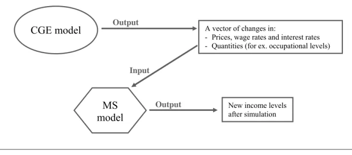
The basic idea is to develop separately a MS model and then to run the simulation on the basis of changes in consumer/producer prices, wages, and sectoral employment levels as predicted by the CGE model. This approach thus uses the two frameworks in a sequential way: first, the policy reform is simulated with the CGE model, and the second step consists of passing the simulated changes in some variables such as prices, wage rates, and employment levels9 down to the MS module, as illustrated in Figure 1.

CGE model

Input

A vector of changes in:

- Prices, wage rates and interest rates - Quantities (for ex. occupational levels)

MS

model

New income levels after simulation

Output

Output

Figure 1 – The Top-Down Approach

9 _{When the assumption of imperfect labour market is adopted, or when the presence of a formal and an informal}

sector is predicted, the rationing in the labour market is usually carried out in the macro or CGE model, while the main use of the MS module is to select those households or individuals who will actually be barred out of, or let in, employment, or the formal sector. We will see this in more detail in the simulation section.

3.1. The Microsimulation Module

The main role of the microsimulation module in the linked framework is to provide a detailed computation of net incomes at the household level, through a detailed description of the tax-benefit system of the economy, and to estimate individual behavioural responses to the policy change. For instance, through the use of microeconometric equations, we can model behav-iours such as labour supply or consumption.

Behavioural Microsimulation (MS) models are developed to capture the possible reactions of the agents to the simulated policies, so that what happens after a reform can be very different from what is predicted by the simple arithmetical computations included in an accounting model.

In this section we will describe in detail a simple behavioural model, following quite closely the discrete labour supply choice model used in Bourguignon et al. (2003b). Another descrip-tion of a similar MS model for labour supply can be found in Bussolo and Lay (2003) with their model for Colombia, and in Hérault (2005), who built a model for the South African economy.

For the building of the model we will use fictitious data describing a very simple economy. In the household survey we have information about some individual characteristics, such as age, sex, level of qualification, education, labour and capital income, the eventual receipt of public transfers, and the activity status. For the sake of simplicity, we have stated that each individual at working age (16-64) can choose between only two alternatives: being a full-time wage worker, or being unoccupied. There are other variables in the survey that are referred to households rather than to individuals, for example the area of residence, the number of house-hold components, the number of adults (over 18 years old) and children (under 18), and so on. All consumption goods of the economy are grouped in two main categories10.

We derive income variables referring to households from initial individual data by summing up individual values for each household member; this way, we obtain households’ labour and capital incomes, households’ public transfers and households’ total income:

10 _{The focus of our distribution and poverty analysis will be on disposable income, even if an inequality and}

where YLmi is labour income of individual i member of household m, YKmi his/her capital

in-come, and TFmi are the public transfers he/she receives from government. All these quantities

are summed up for each family over all the individuals belonging to the family (NCm is the

number of components of household m); then, household m’s total income, Ym, is the sum of

all incomes received by the family: labour income, capital income, and public transfers. For the benchmark situation, we assume all initial prices normalized at one.

Household m’s labour income:

∑

= =NCm i mi m YL YL 1

Household m’s capital income:

∑

= = NCm i mi m YK YK 1

Public transfers to household m:

∑

= = NCm i mi m TF TF 1

Household m’s total income: Y_m =YL_m +YK_m+TF_m

The Model

The core of the behavioural model is represented by the following two equations:

(

)

Log = + ⋅ + ⋅λ + (B.1)

Regression model for log-wage earnings:

Choice of labour market status: W_mi =Ind

[

]

The rest of the MS module is made up by simple arithmetical computations of price indices, incomes, savings and consumption levels. As the parameters entering the following equations (marginal propensity to save mps_m, income tax rates γ, and budget shares η_mq) are constant, this part of the model may be regarded as purely accounting, as it does not contain any possi-ble behavioural response to policy simulations.

Household m’s income generation model: _{m m} NC i mi mi m YL W YK TF Y =

∑

Household disposable (after tax) income: YD_m =

(

)

Household specific consumer price index:

∑

= ⋅ = 2 1 q q mq m P CPI η (B.5)

Real disposable income: YDRm =YDm/CPIm (B.6)

Savings: S_m =mps_m⋅YD_m (B.7)

Household consumption budget: CEBUD_m =YD_m −S_m (B.8)

Consumption expenditure for commodity q: CEmq =ηmq⋅CEBUDm (B.9)

q mq mq P CE C = (B.10)

Consumption level of commodity q:

Household m’s capital income: YKm =PK⋅KSm (B.11)

Description of the subscripts:

m Households m = 1, 2, …, 24

i Individuals belonging to household m i = 1, …, NCm NCm: number of components of household m

q Goods q = 1,2

The first equation of the model, (B.1), computes the logarithm of labour income (wage) of member i of household m as a linear function of his/her personal characteristics (vector includes the logarithm of age, sex, skill level and educational attainment) and of

mi

x

mi

λ , which represents the inverse Mills ratio estimated for the selection model (for more details on the es-timation process see below). The residual term describes the effects of unobserved com-ponents on wage earnings.

mi

v

The second equation represents the choice of the labour status made by household members11. Each individual at working age has to choose between two alternatives: being a wage worker,

11 _{In the literature this kind of equation is known as occupational choice model, or selection model (and also}

dis-crete choice model of labour supply). However, it must be specified that this equation is not really intended to explain the individual choice between being occupied or unemployed, but rather it tries to find out which charac-teristics strengthen the probability of being in one condition rather than in the other one for each individual, as it is described in more detail in the estimation section below.

or being inactive. The variable is a dichotomic variable taking value one if individual i of household m decides to be a wage worker, and zero otherwise. The choice is made by each in-dividual according to some criterion, the value of which is specific to the alternative, and the alternative with the highest criterion value is selected. A natural economic interpretation of this criterion value is utility: each individual chooses the alternative with the highest associ-ated utility. Indeed, we will estimate the selection model using a binomial logit specification, which assigns each individual to the alternative with the highest associated probability. In our model we have arbitrarily set to zero the utility of being inactive. Function “Ind” is an indica-tor function taking value one if the condition is verified, and zero otherwise. Vecindica-tor of ex-planatory variables includes some personal characteristics of individual i of household m, that is: age, sex, skill and educational level, the area of residence and the number of children under 6 living in the household. Variable rw

mi

W

mi

z

mi is the logarithm of real labour income. The equation is

defined only for individuals at working age.

The third equation is an accounting identity that defines total household income, Ym, as the

sum of the wage income of its members YLmi, of the exogenous household capital income

YKm, and of the total amount of public transfers received by household m, TFm. In this

equa-tion, variable Wmi stands for a dummy variable that takes value one if member i is a wage

worker and zero otherwise.

The fourth equation computes household disposable (after tax) income by applying income tax rates according to the rule reported in Table 1. In order to simplify computations, we have assumed that in this economy direct income taxes are imposed on households’ total income

Ym, and not on individual incomes.

Table 1 – Direct Income Tax Rates

Income brackets: Tax rate

Up to 10,000 0%

Up to 15,000 15%

Up to 26,000 24%

Up to 70,000 32%

Over 70,000 39%

Equation (B.5) computes an household specific consumer price index through the consump-tion shares η_mq. Real disposable income is then obtained by dividing households’ disposable income by this index (equation (B.6)).

Then, to find out household m’s savings level, equation (B.7) multiplies this disposable in-come by the marginal propensity to save of each household, . The assumption underly-ing this equation is that household savunderly-ings behaviour is unvaryunderly-ing, as the savunderly-ings level is a fixed fraction of household disposable income. Then, subtracting savings from disposable in-come one obtains the budget that each household spends for consumption (

m

mps

equation (B.8)), which is spent on the two goods of the model according to the budget shares ηmq by equation

(B.9). Again, the assumption in this equation is that consumption behaviour is not flexible, that is, households spend a constant fraction of their consumption budget for each of the two goods.

To get the values of these exogenous parameters (marginal propensity to save and budget shares

m

mps

mq

η ), we use the initial data from the survey in the following way:

m m m YD S mps =

Household m’s marginal propensity to save:

Household m’s consumption budget shares:

m mq mq CEBUD CE = η

Equation (B.10) derives then the consumption levels for each household by dividing the ex-penditure for each good by its price.

Finally, income from capital is obtained by multiplying capital endowment of each family,

KSm, by the return to capital, PK (equation (B.11)).

The initial values of the variables Cmq and KSm (consumption levels and capital endowments,

respectively) are derived from the initial data of the survey by making use of the assumption that in the benchmark situation all prices and returns are equal to one:

Household m’s consumption level of commodity

q: Cmq =CEmq (B.12)

m

m YK

KS = (B.13)

Household m’s capital endowment:

Moreover, we assume that public transfers paid to households and household capital endow-ments are exogenously given. They are fixed at the level reported in the survey, for public transfers, and at the level as computed in equation (B.13), for capital endowment, respectively.

Estimation of the Model

The only two equations in the MS module that need to be estimated are equations (B.1) and

(B.2).

The former, which expresses the logarithm of wage earnings as a linear function of some indi-vidual characteristics and of λmi, the inverse Mills ratio, was estimated using a Heckman

two-step model (see Heckman (1976) and (1979)). We follow this approach to correct for the se-lection bias which is implicit in a wage regression, that is, the fact that we observe a positive wage only for those individuals that are actually employed at the moment of the survey.

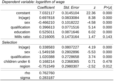
The results of the estimation are reported in Table 2 below. The estimation was conducted on the sub-sample of individuals at working age (16-64).

Table 2 – Heckman selection model, two-step estimates Dependent variable: logarithm of wage

Coefficient Std. Error z P>|z| constant 7.032117 0.3145104 22.36 0.000 ln(age) 0.697818 0.0833084 8.38 0.000 sex -0.466210 0.1018222 -4.58 0.000 qualification 0.396613 0.0771516 5.14 0.000 education 0.525011 0.0871646 6.02 0.000 Mills ratio 0.216005 0.1473164 1.47 0.143 Selection ln(age) 0.338583 0.0807227 4.19 0.000 sex -1.549158 0.2802896 -5.53 0.000 qualification 1.020388 0.2728658 3.74 0.000 children under 6 0.168214 0.2368365 0.71 0.478 region -0.751549 0.2980307 -2.52 0.012 rho 0.762760 sigma 0.283187

The interpretation of the coefficients for the wage equation thus follows that of a simple linear regression. As we can observe in Table 2, age, schooling and skill level have a positive effect on the wage, while being a woman shows a negative effect.

It is important to say that the aim of the wage equation within the model is that of obtaining an efficient estimate for an eventual wage income only for those individuals that are observed to

be inactive in the survey, in the case that, after a policy reform, one or more of them will change their labour market status and become wage workers. In this case, through these esti-mates, we will be able to assign an estimated wage to the individual that has changed his/her labour market status after the simulation run.

For all the other individuals that are observed to receive a wage in the survey, we use instead the observed wage level and not the estimated one.

Parameters of equation (B.2) were obtained through the estimation of a binomial logit model, assuming that the residual terms ε_i are distributed according to the Extreme Value Distribu-tion – Type I12. The estimation was conducted on the sub-sample of individuals at working age (16-64).

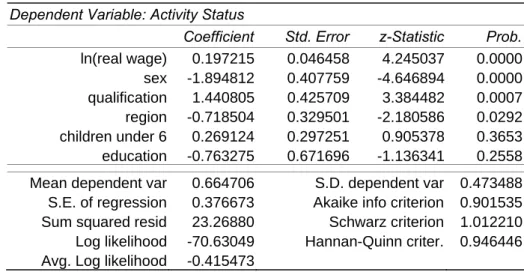
Our explanatory variables include individual characteristics such as the logarithm of predicted real wage, sex, skill and education level, the region of residence and a variable accounting for the presence or not of children under 6 years old in the household. The model is estimated by Maximum Likelihood. Results are presented in Table 3.

Table 3 – Binary logit model for labour status’ choice

Dependent Variable: Activity Status

Coefficient Std. Error z-Statistic Prob.

ln(real wage) 0.197215 0.046458 4.245037 0.0000 sex -1.894812 0.407759 -4.646894 0.0000 qualification 1.440805 0.425709 3.384482 0.0007 region -0.718504 0.329501 -2.180586 0.0292 children under 6 0.269124 0.297251 0.905378 0.3653 education -0.763275 0.671696 -1.136341 0.2558 Mean dependent var 0.664706 S.D. dependent var 0.473488

S.E. of regression 0.376673 Akaike info criterion 0.901535 Sum squared resid 23.26880 Schwarz criterion 1.012210 Log likelihood -70.63049 Hannan-Quinn criter. 0.946446 Avg. Log likelihood -0.415473

12 _{The Extreme Value distribution (Type I) is also known as Gumbel (from the name of the statistician who first}

studied it) or double exponential distribution, and it is a special case of the Fisher-Tippett distribution. It can take two forms: one is based on the smallest extreme and the other on the largest. We will focus on the latter, which is the one of interest for us. The standard Gumbel distribution function (maximum) has the following probability and cumulative density functions, respectively:

(

)

(

)

A binomial model states that the probability of observing the dependent variable assuming value one, given the explanatory variables (OCSmi = 1|Zmi), is equal to the cumulative

distribu-tion funcdistribu-tion of ε_i (the Extreme Value Type I distribution in our case), evaluated at β·Zmi, that

is:

[

]

(

)

The effects that the explanatory variables have on the dependent binomial variable are not lin-ear, because they get channelled through a cumulative distribution function. Thus, by observ-ing the values and signs of the estimated coefficients, we can say somethobserv-ing about the effect that explanatory variables have on the probability that the dependent binomial variable takes value one (wage worker), relatively to the probability that it takes value zero, but not in a lin-ear way.

For instance, expected real wage and qualification seem to influence in a positive way the probability that the dependent variable takes value one (the more qualified the individual is, the higher is the probability for him/her to be employed), as well as the presence of children under 6 does, which is the opposite of what was expected, but anyway this result is not sig-nificant. Moreover, for men the probability of being employed is higher than for women, as the variable SEX, which takes value zero for men and one for women, shows a negative coef-ficient. The same can be said about the region of residence: people living in the first region have a higher probability of being employed than people living in the second one. The vari-able referring to education, instead, seems to have a negative influence on the probability of being employed, which is the opposite of what we expected, and anyway it is not highly sig-nificant.

However, with the estimated coefficients we cannot perfectly predict the true labour market statuses that are actually observed in the survey. Thus, following the procedure described in Duncan and Weeks (1998), we drew a set of error terms ε_i for each individual from the ex-treme value distribution, in order to obtain an estimate that is consistent with the observed ac-tivity or inacac-tivity choices. From these drawn values, we select 100 error terms for each indi-vidual, in such a way that, when adding it to the deterministic part of the model, it perfectly predicts the activity status that is observed in the survey. In other words, the residual term for an individual that is observed to be a wage earner in the survey should be such that:

0 ˆ 6 ˆ ˆ ˆ ˆ ) ( ˆ

ˆ+β₁⋅Log RW_mi +β₂ ⋅SEX_mi +β₃⋅Q_mi +β₄⋅AREA_m +β₅⋅CH _mi +β₆⋅SCH_mi +ε_mi >

α ,

while, for an individual that is observed to be inactive in the survey, the same inequality should be of opposite sign (≤).

After a policy change, only the deterministic part of the model is recomputed. Then, by adding the random error terms previously drawn to the recomputed deterministic component, a prob-ability distribution over the two alternatives (being a wage worker or being inactive) is gener-ated for each individual. This implies that the model does not assign every individual from the sample to one particular choice, but it gives the individual probabilities of being in one condi-tion rather than in the other. This way, the model does not identify a particular choice for each individual after the policy change, but generates a probability distribution over the different alternatives13.

3.2. The CGE Model

The CGE model for the fictitious economy is characterized by a representative household who maximizes a Cobb-Douglas utility function with three arguments: leisure and two consump-tion goods. These commodities are also used as inputs, together with capital and labour, in the production process, which is operated by two firms following a Leontief technology in the ag-gregation of value added and the intermediate composite good, a Constant Elasticity of Substi-tution (CES) function for assembling capital and labour into value added, and a Leontief func-tion in the aggregafunc-tion of intermediate goods. Both factors of producfunc-tion, capital and labour, are mobile among sectors. The capital endowment is exogenously fixed, while labour supply is endogenously determined through household’s utility maximization (subject to fixed time endowment). The wage elasticity of labour supply is estimated from the household survey, in order to have consistency in labour supply behaviour between the two models. Investments are savings-driven, while government maximizes a Cobb-Douglas utility function to buy con-sumption goods and uses labour and capital. The public sector also raises taxes on household’s income and tariffs on imported goods, while it pays transfers to the representative household. For the foreign sector we have adopted the Armington assumption of constant elasticity of substitution for the formation of the composite good (domestic production delivered to domes-tic market plus imports) which is sold on the domesdomes-tic market. Domesdomes-tic production is par-tially delivered to the domestic market and parpar-tially exported, according to a Constant Elastic-ity of Transformation (CET) function. The small country hypothesis is assumed (the economy is price taker in the world market).

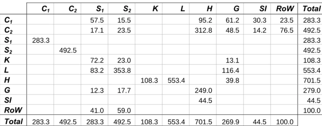
Table 4 – SAM of the Economy C1 C2 S1 S2 K L H G SI RoW Total C1 57.5 15.5 95.2 61.2 30.3 23.5 283.3 C2 17.1 23.5 312.8 48.5 14.2 76.5 492.5 S1 283.3 283.3 S2 492.5 492.5 K 72.2 23.0 13.1 108.3 L 83.2 353.8 116.4 553.4 H 108.3 553.4 39.8 701.5 G 12.3 17.7 249.0 279.0 SI 44.5 44.5 RoW 41.0 59.0 100.0 Total 283.3 492.5 283.3 492.5 108.3 553.4 701.5 269.9 44.5 100.0 Cq: consumption of good q;Sq: sector q; K: capital account; L: labour account; H: representative household

ac-count; G: public sector; SI: savings-investments account, RoW: Rest of the World account.

Table 5 – Values of Parameters for CGE Model

Sector 1 Sector 2

Elasticity of substitution in production function

(ag-gregation of capital and labour) 0.7 0.5

Elasticity of substitution for Armington composite

good 0.7 1.2

Elasticity of transformation for exports and domestic

production delivered to the domestic market -2.0 -3.0 Initial tariff rates on imports 0.3 0.3

Initial time endowment 656.69

Wage elasticity of labour supply

(estimated from the household survey) -0.18665

In the model there are in total 49 variables and 41 equations, which, with the 8 exogenous variables (capital endowment, KS, time endowment, TS, public transfers, TF, the four world prices PWEq and PWMq, and the numeraire, PC), fully determine the model and allow for

sat-isfaction of Walras’ law (we have a redundant equation).

The calibration of the parameters of the CGE model is done on the basis of a Social Account-ing Matrix (SAM) for the economy, in such a way that the benchmark situation is consistent with that of the microsimulation module (for instance, in the benchmark of the two models we have the same average income tax rate, the same average marginal propensity to save, the same budget shares for consumption of the two goods, and so on).

The SAM for the economy under study and the initial values of some other variables are re-ported in Tables 4 and 5, while the equations of the model can be found in Appendix. The data in the SAM are in millions of the monetary unit we have used for the survey.

3.3. Linking the Models

The basic difficulty of this approach is to ensure consistency between the micro and macro levels of analysis. For this reason, one may introduce a system of equations to ensure the achievement of consistency between the two models14. In practice, this consists in imposing the macro results obtained with the CGE model onto the microeconomic level of analysis. In particular:

1) changes in the commodity prices, Pq, must be equal to those resulting from the CGE

model;

2) changes in average earnings with respect to the benchmark in the micro-simulation must be equal to changes in the wage rate obtained with the CGE model;

3) changes in the return to capital of the micro-simulation module must be equal to the same changes observed after the simulation run in the CGE model;

4) changes in the number of wage workers in the micro-simulation model must match those observed in the CGE model.

For our model, these consistency conditions translate into the following set of constraints, which could be called linking equations:

Consumption levels:

(

)

q q q P CE C Δ + = 1 (M.1)

(

)

[

(

)

]

Logarithm of wage

earn-ings: (M.2)

(

)

∑ ∑

∑ ∑

14 _{This way, what happens in the MS module can be made consistent with the CGE modelling by adjusting}

pa-rameters in the MS model, but, from a theoretical point of view, it would be more satisfying to obtain consistency by modelling behaviour identically in the two models.

The variables with no superscripts are those coming from the microsimulation module; those with the ^ notation correspond to the ones that have been estimated: in particular, is the wage level resulting from the regression model for individual i, member of household m, while is the labour market status of individual i of household m deriving from the estima-tion of the binomial choice model.

) ˆ (YL_mi Log mi Wˆ CGE q P

Δ , _ΔPLCGE and _ΔPKCGE _{indicate, respectively, the change in the prices of goods, the}

change in the wage rate and in the return to capital deriving from the simulation run of the CGE model, while parameter _ΔEMPCGE _{is the employment level percentage change from the}

CGE.

WAmi is a dummy variable taking value one if individual i of household m is at working age

(16-64), and zero otherwise. From equation (M.4), the number of employed over the total number of individuals at working age resulting from the MS model must be equal to the change in the employment level observed after the CGE run. This implies that the CGE model determines the employment level of the economy after the simulation, and that the MS model selects which individuals among the inactive persons have the highest probability of becoming employed (if the employment level is increased from the CGE simulation result), or either who, among the wage workers, has the lowest probability of being employed after the policy change (if the employment level is decreased)15.

One possible way of imposing the equality between the two sets of parameters of system of equations (M) is through a change in the parameters of the selection and regression models. Following Bourguignon et al. (2003b), we restrict this change in the parameters to a change in the intercept of the two functions (B.1) and (B.2). The justification for this choice is that it im-plies neutrality of the changes, that is, changing the intercepts a of equations (B.1) just shifts proportionally the estimated wages of all individuals, without causing any change in the rank-ing between one individual and the other. The same applies for the activity status choice equa-tion: we choose to change the intercept α of equation (B.2), and this will shift proportionally all the individual probabilities of being a wage worker, without changing their relative posi-tions in the probability distribution, only to let some more individuals to become employed (or some less if the employment rate of the CGE model is decreased), irrespectively of their per-sonal characteristics. This change in the intercept will be of the amount that is necessary to reach the number of wage workers resulting from the CGE model. Thus, this choice preserves

the ranking of individuals according to their ex-ante probability of being employed, which was previously determined by the estimation of the binomial model. For this reason the change in the intercept parameter satisfies this neutrality property.

4. THE TOP-DOWN/BOTTOM-UP APPROACH

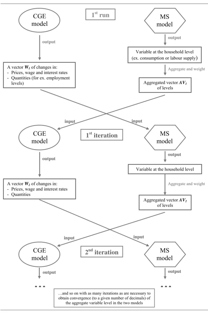
This approach was developed by Savard (2003). It allows overcoming the problem of the lack of consistency between the micro and macro levels of the Top-Down approach by introducing a bi-directional link between the two models: this is the reason why this approach is also called “Top-Down/Bottom-Up”. According to this method, indeed, aggregate results from the MS model (such as consumption levels and/or labour supply) are incorporated into the CGE model, and a loop is used to run both models iteratively until the two produce convergent re-sults.

The value added of this approach is that it takes into account the feedback effects that come from the micro level of analysis, which are instead completely disregarded by the Top-Down model. The basic assumption behind this approach is that the microeconomic effects provided by the MS model run do not correspond to the aggregate behaviours of the representative households used in the CGE model, and that it is thus necessary to take these effects back into the CGE model to fully account for the effects of a simulated policy. A stylized scheme of the way in which this approach works can be observed in Figure 2.

CGE

model

CGE

model

A vector W1 of changes in:

- Prices, wage and interest rates - Quantities (for ex. employment

levels)

Variable at the household level (ex. consumption or labour supply)

Aggregated vector AV1

of levels

Aggregate and weight

output

CGE

model

model

MS

1

run

MS

model

1

iteration

Aggregate and weight

A vector W2 of changes in:

- Prices, wage and interest rates - Quantities

Variable at the household level

Aggregated vector AV2

of levels

…and so on with as many iterations as are necessary to obtain convergence (to a given number of decimals) of

the aggregate variable level in the two models

output

MS

model

2

iteration

…

…

The bilateral communication between the two levels of analysis is achieved through a set of vectors of changes, as in the Top-Down approach: from the macro to the micro level of analy-sis the communication is guaranteed by the changes in the price, wage and return vector and in the employment levels, as before, while from the micro to the macro level the communication we apply two different strategies: in one version, we will use as input for the CGE model a vector of changes in the aggregate consumption and in the labour supply levels from the MS model16; in another version of the same model, only the change in the labour supply level which results from the MS model will be used as input for the CGE model17. The process is then iterated as many times as it is necessary to come to a convergent point, that is, when con-vergence (at a certain number of decimals) is obtained in the aggregate variable levels of the two models.

5. SIMULATION

We will now run a policy simulation with each of the three models. The simulation will be an exogenous shock on the world price level of the good exported by sector 2, which is the labour intensive sector in our stylized economy. The world price of good 2 is reduced of 64 % from its initial value.

16 _{The choice for consumption and labour supply as communicating variables is made following Savard (2003).}

However, as both consumption and labour supply are not exogenous in the CGE model, we have to change some of the initial hypothesis of the model. First, we remove the equations determining consumption demand by the representative household (equation C.1 in Appendix A), substituting them with the following single equation:

. In the initial hypothesis (endogenous consumption) we had 2 endogenous variables (C

∑

2 equations. Now we have 2 exogenous variables and one equation. As we need to insure the balancing of the household’s budget constraint, a variable needs now to be endogenized in the following equation:

(

) (

) (

)

CBUD= 1− ⋅1− ⋅ ⋅ + ⋅ + ⋅ . Following Savard, we choose to endogenize the mar-ginal propensity to save, mps, which is now a variable that changes in order to satisfy the budget constraint. In addition, we introduce an exogenous level of labour supply into the CGE model, and just leave out the equa-tion that determines the demand for leisure (equaequa-tion C.2 in Appendix A). This way, equation C.3 will now yield the demand for leisure as the time remaining after having supplied an exogenous level of labour.

17 _{In this case, we only introduce an exogenous level of labour supply into the CGE model, just leaving out the}

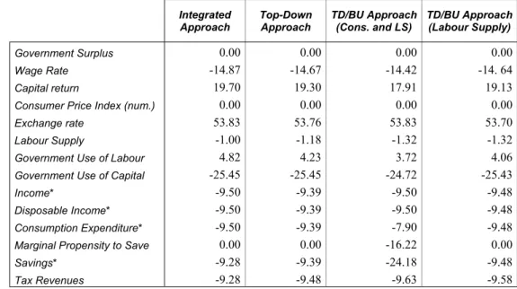
The simulation results for the most relevant macroeconomic variables are reported in percent-age changes in Tables 6 and 7. In the table, also the two different strategies adopted for the TD/BU approach are taken into account, so that we will compare the results coming from the introduction into the CGE model of, respectively, the consumption level and the labour supply coming from the microsimulation module, and only the labour supply.

Table 6 – Simulation Results: Percentage Changes (CGE Model)

Integrated Approach Top-Down Approach TD/BU Approach (Cons. and LS) TD/BU Approach (Labour Supply) 0.00 0.00 0.00 0.00 Government Surplus -14.87 -14.67 -14.42 -14. 64 Wage Rate 19.70 19.30 17.91 19.13 Capital return 0.00 0.00 0.00 0.00

Consumer Price Index (num.)

53.83 53.76 53.83 53.70

Exchange rate

-1.00 -1.18 -1.32 -1.32

Labour Supply

4.82 4.23 3.72 4.06

Government Use of Labour

-25.45 -25.45 -24.72 -25.43

Government Use of Capital

-9.50 -9.39 -9.50 -9.48 Income* -9.50 -9.39 -9.50 -9.48 Disposable Income* -9.50 -9.39 -7.90 -9.48 Consumption Expenditure* 0.00 0.00 -16.22 0.00

Marginal Propensity to Save

-9.28 -9.39 -24.18 -9.48

Savings*

-9.28 -9.48 -9.63 -9.58

Tax Revenues

* _{For the integrated model, these changes are computed as average percentage changes across households.}

Table 7 – Simulation Results: Percentage Changes (CGE Model)

Integrated Ap-proach Top-Down Ap-proach TD/BU Approach (Cons. and LS) TD/BU Approach (Labour Supply) Sector 1 Sector 2 Sector 1 Sector 2 Sector 1 Sector 2 Sector 1 Sector 2

-0.99 0.30 -1.23 0.38 -1.70 0.52 -1.27 0.39 Commodity Prices -8.69 -12.52 -8.81 -12.54 -10.21 -12.05 -8.88 -12.64 Domestic Sales 27.81 -14.20 27.91 -14.31 26.77 -13.86 27.84 -14.43 Domestic Production 43.52 -13.22 43.05 -13.36 41.08 -12.94 42.88 -13.48 Labour Demand 13.07 -26.82 13.14 -26.72 12.72 -25.84 13.15 -26.76 Capital Demand -8.60 -9.78 -8.26 -9.73 -6.58 -8.30 -8.32 -9.84 Consumption* -7.65 -8.84 -8.26 -9.73 -22.87 -24.57 -8.32 -9.84 Investments -32.92 -47.63 -33.11 -47.57 -34.37 -47.21 -33.16 -47.60 Imports 207.36 -78.38 209.23 -78.53 209.10 -78.48 209.11 -78.59 Exports

In general, we can say that we have very similar results for most of the macro variables in all the four simulations. The shock has negative effects on the economy. Indeed, as we can ob-serve in Table 6, the fall in the price of the exported good for sector 2 causes a reduction of the production level for this sector, which reduces its demand for both factors of production. However, due to the depreciation of local currency, the reduction in the local price of the ex-ported good is lower than the 64% world price reduction. For the same reason, exports for the other production sector become convenient, so that for this sector we observe an increase in the level of the exported good, an increase in the production level, and in the demand for capi-tal and labour. The depreciation of local currency has a negative effect on the level of imports, which contributes to a decrease of the amount of goods sold on the domestic market.

The lower level of labour demand as a whole (the second sector is labour-intensive, as can be observed in the SAM, Table 4) generates a reduction in the wage rate, which causes a decrease in labour supply. The opposite is observed for capital, as the first sector is more capital-intensive. As a consequence of the change in the price of the factors, government increases its demand for labour input and decreases the demand for capital, as the latter has become rela-tively more expensive.

As the income of the representative household is based chiefly on the supply of labour, we ob-serve a reduction in nominal income and, as a consequence, of savings and consumption ex-penditure. The amount of consumption goods always decrease, but the percentage change var-ies according to the change in their relative price: the commodity produced by the second sec-tor has become relatively more expensive, due to the negative shock that hit the secsec-tor.

As investments are savings-driven, we observe also a reduction in the demand for investment goods (again, the investment good produced by the second sector is now relatively more ex-pensive, so we observe a higher reduction for the demand of this good).

However, a particular result needs further explanations: savings and investments in the TD/BU-C&LS model decrease much more than in the other three models. The reason for this lays in the fact that, in order to be able to introduce exogenous consumption levels into the CGE model, we must endogenize one variable in the households’ budget constraint to keep the equilibrium in this constraint. Savard’s choice is for the marginal propensity to save, and we follow his approach. But the consequence of this will be a change in the household behav-iour with respect to the initial assumptions made for the benchmark. Indeed, the marginal pro-pensity to save of the household will decrease, and thus also households’ savings. As in our

model investments are savings-driven, this will generate a further reduction of investments. We will analyse this aspect further in the next subsection (5.1).

With respect to the microeconomic results, and mainly the changes in poverty and inequality, we can observe in Table 8 and 9 that the differences are generally significant only for the case of the integrated model.

The underlying variable for the computation of the indices is per-capita real disposable come, obtained by dividing disposable income by the household specific consumer price in-dex18_{, and then dividing it again by the number of adult equivalents resulting by the “Oxford”}

or “Old OECD” scale (see OECD, 1982). This equivalence scale calculates the number of adult equivalents living in a household by assigning a value of 1 to the first household mem-ber, of 0.7 to each additional adult and of 0.5 to each child:

AE = 1 + 0.7⋅(#Adults – 1) + 0.5⋅(#Children).

Table 8 – Inequality Indices on Disposable per Adult Equivalent Real Income (MS Model)

TD/BU Approach (C & LS)* TD/BU Approach (LS)* Benchmark Values Integrated Approach* Top-Down Approach* 33.96 2.81% 1.62% 1.47% 1.60% Gini Index 9.60 4.51% 2.73% 2.48% 2.70% Atkinson’s Index, ε = 0.5 71.80 3.13% 2.29% 2.14% 2.27% Coefficient of Variation

Generalized Entropy Measures:

25.78 6.36% 4.64% 4.32% 4.60%

I(c), c = 2

19.93 3.85% 2.05% 1.81% 2.02%

Mean Logarithmic Deviation, I(0)

20.55 5.17% 3.38% 3.11% 3.34%

Theil Coefficient, I(1)

* _{Percentage deviations from benchmark values.}

First of all, we observe that the Top-Down and the TD/BU-Labour Supply approach show al-most identical results for what concerns both poverty and inequality indices.

The TD/BU-C&LS model we observe a smaller effect on inequality, but in the same direction as for the other two models, and the same is true for poverty.

18 _{The household specific price index is computed using households’ consumption shares and the change in}

prices deriving from the CGE model, as follows:

∑

(

)

= Δ + ⋅ = 2 1 1 q CGE q mq m P CPI η

The biggest difference in the microeconomic results is to be detected in the integrated ap-proach, where we observe a higher increase both in the inequality and poverty indices. The in-crease in inequality for the integrated approach is also confirmed by the higher level of the Severity of Poverty Index, which measures the degree of inequality among the poor, while a higher Poverty Gap Index indicates that the gap between the income of the poor and the pov-erty line has increased (see Appendix B for more details on povpov-erty indices).

Table 9 – Poverty Indices on Disposable per Adult equivalent Real Income (MS Model)

TD/BU Ap-proach (C & LS)* TD/BU Ap-proach (LS)* Benchmark Values Integrated Approach* Top-Down Approach* General Poverty Line

39.34 16.67% 8.33% 8.33% 8.33%

Headcount Index, P0

9.88 40.09% 28.48% 28.07% 28.42%

Poverty Gap Index, P1

0.00 39.99% 29.42% 28.98% 29.36%

Poverty Severity Index, P2

Extreme Poverty Line

4.92 33.33% 33.33% 33.33% 33.33%

Headcount Index, P0

0.96 3.34% 3.18% 3.04% 3.15%

Poverty Gap Index, P1

0.00 -0.36% -0.34% -0.27% -0.34%

Poverty Severity Index, P2

* _{Percentage deviations from benchmark values.}

5.1. More on the TD/BU Approach

In this subsection we want to investigate further what happens within the TD/BU approach in general, and in particular we will try to understand which is the main cause of the unusual de-viation that is observed in the level of savings under the TD/BU-C&LS approach.

At a first intuition, such a deviation could be generated either by a problem of initial data in-consistency between the two datasets (the SAM and the survey), or by what we will refer to as “feedback effects” from the microeconomic level of analysis. With this concept we intend to incorporate all the effects that derive from a response (behavioural or not) of the agents in the MS model that is different from the one observed in the CGE model for the Representative Household (RH). This difference could be due either to a different way of modelling a particu-lar behaviour in the two models (for instance, in the case of labour supply, the MS model uses a discrete and individualized concept of labour supply, while in the CGE model we have a continuous labour supply defined for the RH), or simply to the fact that in the MS model we

consider single households as the unit of modelling, while in the CGE model we have a unique RH (as for consumption and savings, for instance).

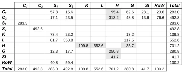
In order to check whether the problem derives from an initial data inconsistency, we will run the same model using a new Social Accounting Matrix, which has been built in such a way that it is fully consistent with the data observed in the survey appropriately aggregated. As we can observe in Table 10, the variables that were adjusted to survey data are those in the grey cells, while all the other columns and rows were then rebalanced to obtain full consistency19. By comparing this SAM with the original one in Table 4, we can observe that in our case ini-tial data inconsistencies were not very big (the biggest inconsistency is observed in the savings level).

Table 10 – SAM of the Economy made consistent with the Household Survey

C S S K L H G SI RoW Total C1 2 1 2 C1 57.8 15.6 95.4 62.6 28.1 23.6 283.0 C2 17.1 23.5 313.2 48.8 13.6 76.6 492.8 S1 283.3 283.0 S2 492.5 492.8 K 73.4 23.2 13.2 109.8 L 81.7 353.8 117.5 552.6 H 109.8 552.6 38.7 701.2 G 12.3 17.7 250.8 280.8 SI 41.7 41.7 RoW 40.8 59.4 100.2 Total 283.0 492.8 283.0 492.8 109.8 552.6 701.2 280.8 41.7 100.2 Cq: consumption of good q;Sq: sector q; K: capital account; L: labour account; H: representative household

ac-count; G: public sector; SI: savings-investments account, RoW: Rest of the World account.

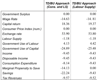
With the SAM shown in Table 10, we will run the shock on the export price of sector 2 as be-fore (-64%). Results are reported in Tables 11 and 12 for the TD/BU-C&LS (consumption and labour supply levels are reported from the MS model into the CGE model) and the TD/BU-LS (only labour supply is reported from the micro level) approaches. Observing the result for sav-ings in the TD/BU-C&LS approach, we can see that in our case data inconsistencies were re-sponsible only for a 2% change in the marginal propensity to save and in the savings level. This means that the remaining change of around 13% (the difference between the change

served in the other approaches, around 9%, and the one observed in this approach, 22.24%) is to be attributed to the feedback effects from the MS model.

Observing the results for the TD/BU-LS approach we discover instead that the change in