CONVERGENCE OF SOLITARY-WAVE SOLUTIONS IN A PERTURBED BI-HAMILTONIAN DYNAMICAL SYSTEM.
II. COMPLEX ANALYTIC BEHAVIOR AND CONVERGENCE TO NON-ANALYTIC SOLUTIONS.
Y. A. Li1 and P. J. Olver1,2
Abstract. In this part, we prove that the solitary wave solutions investigated in part I are extended as analytic functions in the complex plane, except at most countably many branch points and branch lines. We describe in detail how the limiting behavior of the complex sin-gularities allows the creation of non-analytic solutions with corners and/or compact support.
This is the second in a series of two papers investigating the solitary wave solutions of the integrable model wave equation
ut+νuxxt =αux+βuxxx+ 3
νuux+uuxxx + 2uxuxx. (3.6)
(We adopt the notation and numbering of statements from part I.) The ordinary differential equation for travelling wave solutionsu(x, t) =φ(x−ct) is
(α+c)φ′+ (β+cν+φ)φ′′′+ 3
νφφ
′+ 2φ′φ′′ = 0. (3.7)
Substituting φ = φa + a, where a is the undisturbed fluid depth for our solitary wave solutions, and integrating the resulting equation twice, leads to the first order equation
ν(φa+β+cν+a)(φ′a)2 =−φ2a(φa+ 3a+ν(α+c)) (3.17)
To understand why analytic solitary wave solutions converge to non-analytic functions, such as compactons and peakons, having singularities on the real axis, we shall extend the solitary wave solutions described in Theorems 3.1 and 3.2 in Part I to functions defined
1School of Mathematics, University of Minnesota, Minneapolis, MN 55455.
2Research supported in part by NSF Grant DMS 95–00931 and BSF Grant 94–00283.
AMS subject classifications: 34A20, 34C35, 35B65, 58F05, 76B25
in the complex plane to study singularity distribution of these functions. This method not only provides another way to prove the last two theorems, but also makes it clear that singularities of solitary wave solutions are approaching the real axis in the process of convergence. Thus, roughly speaking, the singularities of compactons or peakons come from those complex singularities of analytic solitary wave solutions, which are close to the real axis.
The explicit form (3.3) of solitary wave solutions of the KdV equation shows that they are restriction to the real axis of meromorphic functions with countably many poles in the complex plane so that their analytic extension is unique. In contrast to these functions, extensions of solitary wave solutions under our consideration do not have poles but branch points. These branch points play an important role in the formation of singularities of compactons and peakons. The analytic extension of these solitary wave solutions enables us to understand the loss in analyticity of their limiting compacton or peakon solutions.
For any complex number z ∈C, the real part and the imaginary part of z are denoted byℜz andℑz, respectively. The real partu(x, y) and imaginary partv(x, y) of an analytic function w = F(z) = F(x+iy) = u(x, y) +iv(x, y) will be called the velocity potential and stream function respectively. The level sets of the velocity potential, u(x, y) = u0, and the stream function, v(x, y) = v0, are called the equipotentials and streamlines of F, respectively. Finally, logw is the single-valued branch of the natural logarithmic function Logw, defined as logw= log|w|+iargw with −π <argw≤π.
4. Analytic extensions of solitary wave solutions for ν >0.
We shall consider the solitary wave solutions in Case I , when ν > 0, and Case II , when ν < 0, separately because of their different structures as functions defined on the complex plane. We begin with the compacton case where ν >0. Under the assumption of Theorem 3.1, Equation (3.17) has an orbitally unique and analytic solitary wave solution
φa. Rescaling (3.17) by φa(x) =−ν(α+c+ 3aν )ϕ(x), we reduce it to the equation
(δϕ+ǫ)(ϕ′)2 =ϕ2(1−ϕ), (4.1)
where δ = ν and ǫ = −(β +cν+a)/(α+c+ 3aν ). The phase plane portrait of (4.1) indicates that its solitary wave solutionϕ is a positive, even function with unit amplitude and decaying to zero at infinity. Therefore, as x > 0, the solution ϕ satisfies the integral equation x = Z 1 ϕ 1 ζ s δζ +ǫ 1−ζ dζ = Z 1 ϕ δζ +ǫ ζ dζ p (δζ +ǫ)(1−ζ). 2
Making the substitution
ζ = δ−ǫ 2δ +
δ+ǫ
2δ sinθ, (4.2)
into the preceding integral yields the equation
−x=√ǫ log tan θ 2 + tan θ0 2 1 + tanθ02 tanθ2 + √ δ θ− π 2 , (4.3)
where θ0 is a constant satisfying sinθ0 = δ+ǫδ−ǫ and |θ0| < π2. Equation (4.3) expresses θ implicitly as a function of x, with range −θ0 ≤ θ ≤ π+θ0. Another expression satisfied by the function θ is exp −√1 ǫ x+ √ δ(θ− π 2) = sin θ+θ0 2 cosθ−2θ0. (4.4) We shall use (4.3) and (4.4) to discuss properties of the functionθ in the following lemma. Then the transformation (4.2) will help find extension of the solitary wave solution ϕ to the complex plane.
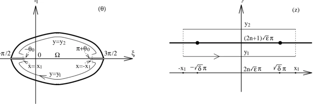
Lemma 4.1. The function θ has an extension Θ(z) which is a holomorphic function on the strip {z ∈C; |ℑz|<√ǫ π}and continuous up to its boundary, such thatΘ(z) maps the
line segment{z =iy; y∈(−√ǫ π,√ǫ π)} onto the line segment{θ = π2+iη; η ∈(−ηǫ, ηǫ)}
with Θ(i√ǫ π) = π2 −iηǫ, Θ(0) = π2 and Θ(−i√ǫ π) = π2 +iηǫ for some ηǫ >0.
Proof. If we consider the right-hand side of (4.3) as a function of θ, denoted by −Σ(θ), then Σ(θ) maps the interval (−θ0, π +θ0) homeomorphically onto the real axis R with Σ(−θ0) =∞, Σ(π2) = 0 and Σ(π+θ0) =−∞. Substituting θ = π2+iη into the right-hand side of Equation (4.3) to extend the function Σ to the line{θ = π2 +iη; η∈R}, it follows that Σ π 2 +iη =−i √ δ η+ 2√ǫtan−1 r ǫ δ tanh η 2 , (4.5)
which indicates that iΣ(π2 +iη) is an odd and increasing function of η, mapping the real axis to itself homeomorphically. In consequence, Θ maps{z =iy; y ∈[0,√ǫπ]}to the line segment{θ = π2+iη; η∈[−ηǫ,0]}and it maps{z =iy; y ∈[−√ǫπ,0]}to the line segment
{θ = π2 +iη; η ∈[0, ηǫ]}, where Σ(π2 +iηǫ) =−i√ǫπ.
Replacing x with x+iy and substituting θ = ξ +iη into Equation (4.4), one obtains the equation
sinθ0coshη+ sinξ+icosθ0sinhη
coshη+ cos(ξ−θ0) = exp
−1 √ ǫ x+ √ δ(ξ− π 2) +i(y+ √ δη) . (4.6)
Comparing norms and angles on both sides of (4.6) leads to the equations, coshη−cos (ξ+θ0) coshη+ cos (ξ−θ0) = exp −√2ǫ x+√δ(ξ− π 2) , (4.7) and
sinξ =−sinθ0coshη−cosθ0sinhηcot
y+√δη √
ǫ . (4.8)
For each y∈ (0,√ǫ π), the graph of the streamline (4.8) is symmetric with respect to the line{π2 +iη;η∈R} and is the reflection of the streamline for y=−y0 with respect to the real axis. Moreover, Σ is a one-to-one mapping of the streamline connecting the points (−θ0,0) and (π +θ0,0) in the lower-half plane onto the line {x+iy0;x ∈ R} for each
y0 ∈ (0,√ǫπ) with Σ(π +θ0) = −∞+iy0, Σ(π2 +iη0) = iy0 and Σ(−θ0) = ∞+iy0. The streamline √ǫπ = y(ξ, η) of the function Σ, consisting of the line segments {ξ; ξ ∈
[−π2,−θ0)} and {ξ; ξ ∈(π+θ0,3π2 ]} and the curve in the lower-half plane connecting the points (−π2,0) and (3π2 ,0) as shown in Figure 7, is homeomorphic to the line{x+i√ǫπ;x∈
R}. Whereas for each x0 ∈R, the equipotential x(ξ, η) =x0 is symmetric with respect to the ξ-axis, and it is the reflection of the equipotential x(ξ, η) = −x0 with respect to the lineξ =π/2. Furthermore, Σ maps the equipotential x=x(ξ, η) homeomorphically to the line {x+iy; y ∈ (−∞,∞)} for each fixed x ∈ (0,√δ π) with Σ(π2 − √x
δ −i∞) = x+i∞ and Σ(π2 − √x
δ +i∞) = x−i∞. Also, Σ is a one-to-one mapping of the equipotential
x=x(ξ, η) onto the line segment {x+iy;y ∈(−√ǫ π,√ǫ π)} for each x∈[√δ π,∞).
−θ0 (θ) y 0 − π − ε π π −π /2 π /2 π+θ0 x (z) ξ Ω 3π δ ε /2 δ π
Fig. 7. Streamlines and equipotentials of the function z = Σ(θ)
As a result of the above discussion, the function Σ(θ) is seen as a conformal mapping of the domain Ω onto the strip{x+iy; −∞< x <∞,|y|<√ǫ π}, where Ω is bounded above
by the streamline −√ǫ π =y(ξ, η) consisting of the line segments {ξ; ξ ∈[−π2,−θ0)} and
{ξ;ξ ∈(π+θ0,3π2 )}, and the thickest solid curve in the upper-half plane shown in Figure 7, and Ω is bounded below by the streamline√ǫ π =y(ξ, η) also consisting of the line segments
{ξ;ξ ∈[−π2,−θ0)}and{ξ; ξ ∈(π+θ0,3π2 )}, as well as the thickest solid curve in the lower-half plane illustrated in Figure 7. Therefore, the inverse θ(x) of the the function Σ(θ) has an analytic extension Θ(z) to the strip{x+iy; −∞< x <∞,|y|<√ǫ π} and continuous up to its boundary ([3], Thm. 14.18). Then the transformation ϕ= δ2δ−ǫ + δ+ǫ2δ sinθ leads to the conclusion that the solitary wave solution ϕ of (4.1) has an analytic extension to
the same strip.
An immediate consequence of Lemma 4.1 is the existence of a cuspon as a weak solution of Equation (4.1). When η = 0, y = √ǫ π and −π2 < ξ < −θ0, it follows from (4.6) that the equation sinξ+ sinθ0 1 + cos(ξ−θ0) =−e−√1ǫ x+ √ δ(ξ−π 2) . (4.9)
implicitly determines the value of the function Σ on the line segment {ξ;ξ ∈(−π2,−θ0)} which is mapped to the line{x+i√ǫ π; x∈(√δ π,∞)}. Extending the function Σ on the real axis from ξ = −π2 to the left up to the point ξ = −π +θ0, one may also realize that Σ maps{ξ; ξ ∈(−π+θ0,−θ0)} homeomorphically to the line {x+i√ǫ π; x∈(−∞,∞)}. This leads us to the discovery of the cuspon solution of Equation (4.1), as stated in the following corollary.
Corollary 4.2. Equation (4.1) has a weak solution ϕp in the sense of Definition 3.1.
Moreover, ϕp is an even and negative function, continuous on the real axis, monotonically
increasing on the positive x-axis and approaching zero at infinity, thereby representing a wave of depression. The derivativeϕ′
p has a discontinuity at the minimum of ϕp.
Proof. It follows from (4.9) that the equation
x=−√δ(ξ− π
2)−
√
ǫlog −(sinξ+ sinθ0) 1 + cos(ξ−θ0)
determines a function ofξ, denoted by x= Σp(ξ) for −π+θ0 < ξ <−θ0. Since
dx dξ =− √ δ(sinξ+ 1) sinξ+ sinθ0 , (4.10) dx
dξ >0 on the interval (−π+θ0,−θ0), and thus Σp is an increasing function whose graph is symmetric with respect to the point (−π2,√δ π), having an inflection point at ξ = −π2
and asymptotes ξ = −π +θ0 and ξ = −θ0. Therefore, the inverse of Σp, denoted by
ξ = ξ(x), is also an increasing function, symmetric with respect to the point (√δ π,−π2) with ξ′(√δ π) =∞. Let ϕp(x) = δ−ǫ 2δ + δ+ǫ 2δ sin ξ(x+ √ δπ) . (4.11)
Because of the symmetry −π −ξ(x) = ξ(2√δ π−x), we see that ϕp is an even function having a cusp atx= 0 such that lim
x→0−ϕ ′ p(x) =−∞and lim x→0+ϕ ′ p(x) =∞. Moreover, ϕp is continuous. Then the translation invariance of Equation (4.1) shows that ϕp is the cuspon solution satisfying properties stated in this lemma. It is also worth noticing that so called “cuspon solution” in this case is represented by two unbounded orbits illustrated in Figure
2.
In order to find further extension of Θ(z), we need to study other properties of the function Σ defined on the complex plane, such as its singularities, streamlines y =y(ξ, η) for |y| >√ǫ π and zeros of its derivative given by (4.10). We summarize these properties as follows.
(i) Singularities of Σ and zeros of dΣdθ. There are two countable sets of distinguished points on the ξ axis: the critical points where dΣdθ = 0, and so Σ is not angle-preserving occur at O = {−π2 + 2nπ; n = 0,±1,±2,· · · }. The singularities of Σ are at S = {−θ0+ 2nπ, θ0+ (2n+ 1)π; n= 0,±1,±2,· · · }. Let Γ+ (respectively Γ−) be a closed Jordan curve
containing only the singular pointξ =θ0+ (2n+ 1)π (respectivelyξ =−θ0+ 2nπ), but no other points inS. Integrating dΣdθ once around Γ± in the counterclockwise direction yields
Z Γ±− √ δ(sinξ+ 1) sinξ+ sinθ0 dξ =±i2π√ǫ.
Therefore, singularities of Σ are branch points of infinite order.
(ii) A single-valued branch Σ0 of Σ. Notice that if we integrate dΣdξ on a closed path Γ2 whose interior contains only two adjacent singularities (2n−1)π+θ0 and 2nπ−θ0 of Σ for some integer n, then
Z Γ2− √ δ(sinξ+ 1) sinξ+ sinθ0 dξ =−i2π√ǫ+i2π√ǫ= 0,
i.e. the value of the function Σ does not change after a complete circuit around the two singular points (2n−1)π +θ0 and 2nπ−θ0. Therefore, to find a single-valued branch
Σ0 of the multi-valued function Σ, one may define countably many branch lines on the
ξ-axis by {ξ; (2n−1)π+θ0 ≤ ξ ≤ 2nπ−θ0} for n = 0,±1,±2,· · ·. Let Σ0 be defined to take the same value as the function Σ on the domain Ω bounded by the streamlines
−√ǫ π =y(ξ, η) and √ǫ π =y(ξ, η), and contained in the strip {ξ+iη; −π2 < ξ < 3π2 , η ∈
R} as illustrated in Figure 7. Then using the property that x+iy = Σ(ξ+ iη) if and only if x−2nπ√δ+iy = Σ(ξ+iη+ 2nπ), one can extend the function Σ0 to the domain Ωn = {ξ + iη + 2nπ; ξ +iη ∈ Ω} for n = ±1,±2,· · ·. To get a complete portrait of the function Σ0, let us consider its streamlines y0 = y(ξ, η) for |y0| > √ǫ π. Using an argument similar to that used to consider the streamline √ǫ π = y(ξ, η), one may show that the streamline is decreasing on the interval (−π2,π2) and increasing on the interval (π2,3π2 ) with η′(−π
2) = η′( π
2) = η′( 3π
2 ) = 0, where η is a function of ξ determined by the streamline (4.8) and η(π2) is determined by the equation y0 = −iΣ0 π2 +iη
as shown in (4.5). Then the property of the stream function y(ξ, η) = y(ξ+ 2π, η) shows that for each
y0 ∈(−∞,−√ǫ π)∪(√ǫ π,∞), the streamline y0 =y(ξ, η) determines a functionη =η(ξ) defined on the real axis such thatη(ξ) is a continuous and periodic function with the period 2π. Using the Cauchy-Riemann equations for x andy leads to the conclusion that Σ0 is a one-to-one mapping of the streamliney0 =y(ξ, η) onto the line y=y0.
Remark. For any integer n, we find that Σ maps Ωn onto the strip {|ℑz| < √ǫ π},. Therefore Σ can be defined as a conformal mapping from a Riemann surface obtained by excluding Ωn, n = ±1,±2,· · ·, onto a domain containing the strip {|ℑz| < √ǫ π}, whose inverse is the extension of the function Θ(z) defined in Lemma 4.1. It is also important to realize that Θ(z) has four singularities on the boundary of the strip {|ℑz| < √ǫ π}, even though Θ can be extended up to the boundary continuously. We demonstrate this fact in the following lemma.
x = x y=y x = 2δ π ε y = 2 π x = x0 π y = 2επ δ x = 2 ξ π ε − π ε π δ 0 (z) y x (θ) 0 0 0 0 0 y=y0 -y -y x -x -x0 −5π/2 3π/2 0 δ x = 2 π -x0 y = 2 0 ε π-y0 y=y0 η y0 0 x = x
Fig. 8. A sketch of the path γ in the θ-plane and the corresponding path Σ(γ) in the z-plane
Lemma 4.3. √δ π±i√ǫ π and −√δ π±i√ǫ π are singularities of the function Θ(z) and each of them is a branch point of order three.
Proof. We choose a closed path γ consisting of segments of streamlines and equipotentials of Σ in the θ-plane, as illustrated in Figure 8, which starts from the point θ =ξ0+iη0 on the streamline y0 = y(ξ, η) such that −π2 < ξ0 < 0, η0 < 0, x0+iy0 = Σ0(ξ0+iη0) with 0< x0 <
√
δ πand 0< y0 <√ǫ π, and both
√
δ π−x0and√ǫ π−y0 are sufficiently small. If one goes along the pathγ counterclockwise for a complete circuit, then the corresponding trace described by the function Σ in the z-plane finishes three complete circuits of the rectangle Σ(γ). Since the pathγ is contained in the strip {ξ+iη; −π < ξ <0, η ∈R}, and sine function sinθ has the period 2π, √δ π+i√ǫ π is also a branch point of order three of the function ϕ= δ+ǫ2δ (sin Θ + sinθ0). In the similar way, one may show that the other three points √δ π−i√ǫ π and−√δ π±i√ǫ π are also branch points of order three of both
functions Θ and ϕ.
One may also question whether Θ has other singularities on the lines{x±i√ǫ π; x∈R}. As a matter of fact, it follows from the derivative of Σ shown in (4.10) and the streamlines
−√ǫ π = y(ξ, η) and √ǫ π = y(ξ, η) portrayed in Figure 7 that Θ(z) has a local analytic extension from the interior of the strip {z ∈ C;|ℑz| < √ǫ π} to each point on the lines
{x+i√ǫ π; x ∈ R} and {x−i√ǫ π; x ∈ R} except the four branch points √δ π±i√ǫ π and−√δ π±i√ǫ π. Therefore, to extend Θ(z) beyond these two lines, one needs to define branch lines connecting these branch points. Different definitions of branch lines lead to different extensions of Θ to the complex plane. In the following theorems, we discuss two distinct extensions of Θ(z) beyond the strip {z ∈C;|ℑz| ≤√ǫ π}.
Theorem 4.4. Let Σ0 be the single-valued branch of Σ defined in (ii), and let
D0 =
[
n6=0
Ωn∪ {ξ;−∞< ξ ≤ −θ0} ∪ {ξ; π+θ0 ≤ξ <∞},
where Ωn is the same as defined in (ii). Then the restriction of Σ0 to the domain X0 = C\D0 is a conformal mapping of X0 onto the domain
Y0 =C\ {x+i√ǫ π; |x| ≥
√
δ π} ∪ {x−i√ǫ π; |x| ≥√δ π} ,
and the inverse Θ0 of the function Σ0 is an analytic extension of Θ(z) to the manifold
Y0 such that Θ0(z) has countably many branch points (2k + 1)
√
δ π±i√ǫ π for integers k = 0,±1,±2· · · and when k 6=−1,0, the singularities(2k+ 1)√δ π±i√ǫ π are located at
the upper side of the branch line {x+i√ǫ π;|x| ≥√δ π} and the lower side of the branch line {x−i√ǫ π; |x| ≥√δ π}, satisfying Θ0 (2k+ 1)
√
δ π±i√ǫ π
=−(2k+ 1)π+ π2. Proof. It follows from Lemma 4.1 an the discussion in (ii) that Σ0|X0 is a one-to-one mapping of X0 onto Y0. Therefore, the inverse of Σ0|X0, denoted by Θ0(z), is an analytic function on Y0, and its restriction to the strip {x+iy; x∈R,|y|<√ǫ π} is Θ(z).
Theorem 4.5. Let Y1 = C\
∞
S
n=−∞{
x+i√ǫ(2n+ 1)π; |x| ≤ √δ π}, and let X1 be the
Riemann surface formed by infinitely many layers of the domainΩ defined in Lemma 4.1, having branch lines{ξ;−π2 ≤ξ ≤ −θ0} and {ξ;π+θ0 ≤ξ ≤ 3π2 }, and being pasted in such
a way that on any layer of the Riemann surface, if one goes across any of the two branch lines from the lower half plane, one gets to the next lower layer of the Riemann surface; whereas if one goes across any of the branch lines from the upper-half plane, one arrives at the adjacent upper layer of the Riemann surface. Then there exists a conformal mapping of X1 onto the Riemann surface Y1 such that its inverse Θ1 is an analytic extension of Θ from the strip {x + iy; x ∈ R,|y| < √ǫ π} to Y1, and Θ1 is continuous up to the
boundary of Y1. Moreover, Θ1 has infinitely many branch points ±
√
δ π+i(2n+ 1)√ǫ π for n = 0,±1,±2,· · ·, such that each pair of branch points ±√δ π+ i(2n+ 1)√ǫ π are connected by the branch line bn = {x+i(2n+ 1)√ǫ π; |x| ≤
√
δ π} which is regarded as a line segment having an upper side and a lower side.
/2 −π 0 3π/2 η (θ) y (z) ξ y=y1 x= θ π+ −θ0 Ω x y x 0 1 π δ − δ π 1 x=-x x1 -x1 (2n+1) y y=y 1 2 2 ε π 2n επ
Fig. 9. A sketch of the path γ1 in the θ-plane and the corresponding path Σ(γ1) in thez-plane
Proof. It follows from Lemma 4.1 and (ii) that Θ is a homeomorphism of the strip {x+
iy; x ∈ R,|y| <√ǫ π} onto Ω, whose inverse is a branch Σ0 of the function Σ. There are also countably many other branches of Σ, denoted by Σn for n = ±1,±2,· · ·, such that
Σn(θ) = Σ0(θ) +i2√ǫ nπ for any θ ∈ Ω and Σn is a homeomorphism of Ωn = Ω onto the strip Sn = {z ∈ C; (2n−1)√ǫ π < ℑz < (2n+ 1)√ǫ π}. If one chooses a path, denoted byγ1 as shown in Figure 9, and extends the value of Σn by starting from a point on γ1 in the lower half plane, going clockwise along γ1 and coming back to the same point after a complete circuit, then the corresponding values of Σnform a complete circuit of a rectangle in the z-plane. Therefore, if one defines the branch line {x+i(2n+ 1)√ǫ π,|x| ≤√δ π}, then one may extend the inverse Σ−n1 of Σn from the stripSn to to the stripSn+1 uniquely and analytically. Hence, we may use the domain Ωn of the branch Σn to construct the Riemann surfaceX1 for Σ and obtain a conformal mapping ofX1 ontoY1 (ref. [1] ), whose inverse Θ1 is an analytic extension of Θ to the domain Y1.
Remark. It follows from the definition of the function Θ1 in the last theorem that Θ1 can also be regarded as a periodic function with the period T = i2√ǫ π, mapping each strip Sn homeomorphically onto the domain Ω. In Section 6, we will use this property to discuss how solitary wave solutions extended as analytic functions defined on a Riemann surface converge to either a compacton or a solitary wave solution of the KdV equation as
ǫ or δ approaches zero.
5. Analytic extensions of solitary wave solutions for ν <0.
As we have seen in Section 3, the dynamical structure of Equation (1.1) changes notice-ably when the sign of the parameterνchanges from positive to negative. In this section, we shall show that solitary wave solutions in caseν <0 have a different singularity distribution from the solitary wave solutions in case ν >0.
Suppose that the coefficients of Equation (3.17) satisfy the conditions
−(β+cν)<−ν
3(α+c)< a < 1
2(β−να) and ν <0.
Then (3.17) has an orbitally unique and analytic solitary wave solution φa defined on the real axis as demonstrated in Section 3. Rescaling (3.17) by the transformation φa = [3a+ν(α+c)]ϕ reduces it to the equation
(δϕ+ρ)(ϕ′)2 =ϕ2(ϕ+ 1), (5.1)
where δ=−ν >0, ρ= −3a+ν(α+c)ν(β+cν+a) > δ. Then the corresponding solitary wave solution of (5.1) is symmetric with respect to its depression, having the amplitudeA = 1 with ϕ <0 and monotonically approaching zero at infinity. Since solutions to (5.1) are translation invariant, without loss of generality, we let the solitary wave solutionϕbe an even function,
which satisfies the integral equation −x =Rϕ −1 √ δϕ+ρ dϕ ϕ√ϕ+1 for x≥0. Substituting ϕ= ρ−δ 2δ cosht− ρ+δ 2δ (5.2)
into the above integral yields the following expressions
−x = Z t 0 √ δ(cosht+ 1) cosht−cosht0 dt=√δ t+√ρlogtanh t0 2 −tanh t 2 tanht02 + tanh2t, (5.3)
where cosht0 = ρ+δρ−δ, t0 >0. Let
∆(t) =− √ δ t+√ρlogtanh t0 2 −tanh2t tanht02 + tanh2t . (5.4)
We shall extend the function ∆ to the complex plane, which in turn will provide information to find an analytic extension of the inverse t= Ξ(x) of ∆, satisfying Equation (5.3).
Since tanht02 −tanh t 2 tanht02 + tanh2t =e −x+√δt √ρ ,
replacingt and x withξ+iη andx+iy in the above equation, respectively, and rewriting its left-hand side as a sum of its real part and imaginary part, one obtains
cosht0cosη−coshξ−isinht0sinη cosh(t0+ξ)−cosη =e−x+ √ δξ+i(y+√δη) √ρ .
Comparing angles and norms on both sides of this equation yields the two relations sinht0sinη
cosht0cosη−coshξ
= tany+
√ δ η
√ρ , and cosh(t0−ξ)−cosη cosh(t0+ξ)−cosη
=e−2(
x+√δ ξ) √ρ
,
which provide equations of streamlines and equipotentials of the function ∆, respectively. Similar to the technique used to study the function Σ, starting from the imaginary axis
t=iη to extend ∆(t), one has the expression
y=−i∆(iη) =−√δ η+√ρ2nπ+ 2√ρtan−1 r ρ δ tan η 2 , (5.5)
for anyη∈ (2n−1)π,(2n+1)πwithn= 0,±1,±2,· · ·, which leads to the determination of streamlines y0 = y(ξ, η) of the function ∆. As illustrated in Figure 10, when y0 ∈ (−(√ρ−√δ)π,(√ρ−√δ)π), the streamliney0 =y(ξ, η) is a smooth curve connecting the points −t0 and t0 on the ξ-axis, and ∆ maps the streamline diffeomorphically to the line
{x+iy0, x∈R}, on which ∆(−t0) =−∞+iy0, ∆(iη0) =iy0, and ∆(t0) =∞+iy0, where
y0 and η0 satisfy (5.5) with n = 0. If y0 = (√ρ−
√
δ)π, the streamline is a curve in the upper-half plane connecting pointst=−t0, πiand t0, having a corner at the pointt =πi, and ∆ is a homeomorphism of this streamline to the line{x+i(√ρ−√δ)π; x∈R}. On the other hand, fory0 =−(√ρ−
√
δ)π, the streamline is a curve symmetric to the streamline for y0 = (√ρ −
√
δ)π with respect to the ξ-axis. For each x0 > 0, the equipotential
x0 = x(ξ, η) is a closed loop in the right-half plane which starts from a point to the right of the pointt0 on the ξ-axis, going aroundt0 clockwise once for a complete circuit. In this way, ∆ is a one-to-one map of the equipotential onto the line segment{x0+iy; |y|<√ρπ}; while the equipotential −x0 =x(ξ, η) is symmetric to the equipotential x0 =x(ξ, η) with respect to the η-axis. Since the proof of these facts and the following lemma concerning analytic extensions of ∆ and its inverse function is similar to that of Lemma 4.1, we omit it to avoid tedious details here.
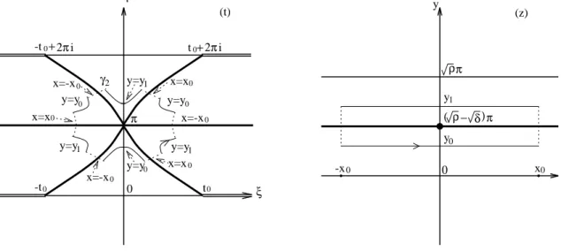
Lemma 5.1. Let ∆ be the function defined in (5.4). Then as a homeomorphism of the line segment {ξ; −t0 < ξ < t0} onto the real axis, ∆ has an analytic extension to the
region D bounded by the streamline (√ρ−√δ)π = y(ξ, η), connecting points t = −t0, πi
and t0, and the streamline−(√ρ−
√
δ)π =y(ξ, η), connecting points t=−t0,−πiand t0.
Moreover, the extension of ∆ is a one-to-one mapping of D onto the strip
S0 ={x+iy; x∈R,|y|<(√ρ−
√ δ)π},
whose inverse t = Ξ(z) is an analytic function defined on the strip S0 and continuous up
to its boundary such that t = Ξ(z) satisfies Equation (5.3). In consequence, the transfor-mation (5.2) leads to the analytic extension of the solitary wave solution ϕ of (5.1) to the strip S0 as well.
In analogy with the discussion of solitary wave solutions in Section 4, we now summarize properties of the function ∆, including its singularities, critical points, and single-valued branches. This will lead us to find singularities of the function Ξ on the boundary of the trip S0 and its further extension to the complex plane.
(a) Singularities of ∆ and zeros of d∆dt . Clearly ∆ has singularities t = ±t0+ 2nπi for
n= 0,±1,±2,· · ·. Let L+ be a Jordan curve whose interior contains only one singularity
t=t0+ 2nπiof ∆ for some integer n, and let L− be a closed path whose interior contains
only the singularity t=−t0+ 2nπiof ∆. Integrating d∆dt along these curves yields
Z L± d∆ dt dt= Z L± √ δ(cosht+ 1) cosht0−cosht dt=∓2π√ρ i. 12
ξ η π −π 0 − ρ δ)π x ρπ y − ρπ ρ− ( − δ π) (z) 0 (t) D F _ F+ E+ 0 -t t0 E_ (
Fig. 10. Streamlines and equipotentials of the function ∆ when δ < ρ≤3δ
Therefore, t=±t0+2nπiare branch points of infinite order of ∆, and thus ∆ is a multi-valued function. On the other hand, zeros of d∆dt are t= (2k+ 1)πi for k = 0,±1,±2,· · ·, and ∆ is not angle-preserving at these points. As illustrated in Figure 10, the streamlines (√ρ−√δ)π =y(ξ, η) and −(√ρ−√δ)π =y(ξ, η) joining the pointst =±t0 and forming the boundary of the regionDhave corners att=πiandt =−πi, respectively. As a matter of fact, ∆ is not one-to-one in some neighbourhood of these points either, because η =πi
is also the streamline (√ρ−√δ)π = y(ξ, η) such that ∆(−∞+πi) =∞+ (√ρ−√δ)πi, ∆(πi) = (√ρ−√δ)πi and ∆(∞+πi) = −∞+ (√ρ−√δ)πi; while η = −πi is another streamline−(√ρ−√δ)π =y(ξ, η) such that ∆(−∞ −πi) =∞ −(√ρ−√δ)πi, ∆(−πi) =
−(√ρ−√δ)πiand ∆(∞ −πi) =−∞ −(√ρ−√δ)πi, which indicates that the open set we shall seek and use to construct the Riemann surface on which ∆ is a conformal mapping has to be contained in the strip {ξ+η; ξ ∈R,|η|< π}.
(b)A single-valued branch∆0 of∆. Since ∆ has branch points±t0+2nπi, first of all, we define branch lines byln={ξ+2nπi; |ξ| ≥t0}forn= 0,±1,±2,· · ·, so that the integration of d∆dt along any closed path contained in the open setL=C\ ∞∪
−∞lnis zero,i.e. values of the
function ∆0 can be uniquely determined on the domainL. BecauseD⊂L, the function ∆0 is shown to be a homeomorphism ofD onto the stripS0 in Lemma 5.1, whose streamlines and equipotentials are sketched in Figure 10. It is worth mentioning that in Figure 10 the curve E− connecting the point t = −πi and a point to the right of t = t0 is part of the equipotential 0 = x(ξ, η) such that ∆0(E−) = {iy; −√ρ π < y < −(√ρ−
√ δ)π}, and the curve E+ symmetric to E− with respect to the ξ-axis is also a portion of the
{iy; (√ρ−√δ)π < y <√ρ π}. On the other hand, the curves F− and F+ symmetric to
E− and E+ with respect to the imaginary axis have the same image as E− and E+, respectively, i.e. both E− ∪ {iη; |η| ≤ π} ∪ E+ and F− ∪ {iη; |η| ≤ π} ∪ F+ are the equipotential 0 = x(ξ, η) such that ∆0 maps each of them homeomorphically onto the line segment {iy; |y| ≤ √ρ π}. In addition, solid lines passing through the curves E+ and F+ in Figure 10 are streamlines y0 = y(ξ, η) for some y0 ∈ ((√ρ −
√
δ)π,√ρ π), and solid lines passing through the curves E− and F− are streamlines y0 = y(ξ, η) for some y0 ∈ (−√ρ π,−(√ρ−
√
δ)π). For each of them, ∆0 is a homeomorphism onto the line {x +iy0; x ∈ R}. Dotted and dashed lines to the right of curves E− and E+ are equipotentials x0 = x(ξ, η) for some x0 < 0, which are mapped homeomorphically onto the lines {x0+iy; −√ρ π < y <−(√ρ−
√
δ)π} and {x0+iy; (√ρ−
√
δ)π < y < √ρ π}, respectively. Symmetrically, dotted and dashed lines to the left of curves F− and F+ are equipotentials x0 = x(ξ, η) for some x0 > 0, whose images are also line segments
{x0+iy; −√ρ π < y < −(√ρ−
√
δ)π}and{x0+iy; (√ρ−
√
δ)π < y <√ρ π}, respectively. Before finding a further extension of the function Ξ beyond the strip S0, we need to point out in the following lemma that Ξ has singularities on the boundary of S0, which has an effect on how to determine a further extension for Ξ.
0 -t0 η +2πi -t0+2πi y=y0 0 y=y1 x=x0 y=y 0 0 y=y 0 x=x 0 y=y ( ρ− δ) y π y y 0 1 x0 0 ρπ 0 -x π t0 x=-x x=x x=-x (t) (z) ξ x y=y1 0 1 0 t 0 x=-x γ2
Fig. 11. The path γ2 and the corresponding rectangle in the z-plane
Lemma 5.2. The function Ξ has singularities at z = ±i(√ρ−√δ)π which are branch points of order three.
Proof. Since Ξ (√ρ−√δ)πi
=πi and Ξ|S0 = (∆0|D)−1, to show that z = (
√ρ−√δ)πi
is a branch point of Ξ, we choose a closed path γ2 consisting of segments of streamlines and equipotentials of the single-valued branch ∆0 such that its interior contains t = πi as sketched in Figure 11. As t moves around the circuit γ2 once in a counterclockwise direction, its image ∆0(t) traces three complete circuits of a rectangle in the z-plane with its interior containing the pointz = (√ρ−√δ)πi. It follows that the pointz = (√ρ−√δ)πi
is a branch point of order three of the function Ξ. Noticing that cosht is a periodic function with the period T = 2πi, the solitary wave solution to (5.1) is given by the transformationϕ= ρ2δ−δ(cosht−cosht0) witht = Ξ(z) and the pathγ2 is contained in the strip {ξ+iη; ξ ∈ R,π
2 < η < 3π2 }, one concludes that z = (
√ρ
−√δ)πi is also a branch point of order three of the solitary wave solutionϕ. The proof thatz =−(√ρ−√δ)πi is
a branch point of order three is similar.
It follows from Lemma 5.2 that any extension of solitary wave solutions of Equation (5.1) beyond the stripS0will depend on how branch lines are defined in the complex plane. In the following theorems, we give two different definitions of branch lines and consequent extensions of Ξ(z).
Theorem 5.3. Let D0 be the open set bounded by the curves E±, F± and branch lines
s+ ={t =ξ; t0 ≤ξ ≤ ξ0} and s− ={t =ξ; −ξ0 ≤ ξ ≤ −t0}, where ξ0 is the intersection
of E+ and the ξ-axis as shown in Figure 12. Then the function t = Ξ(z) has a further
extension t = Ξ1(z) to the domain
Y1 =C\ ∞ [ n=−∞ {iy; (2n+ 1)√ρ−√δ π ≤y ≤ (2n+ 1)√ρ+√δ π},
such that t = Ξ1(z) is a homeomorphism of the open set
En={x+iy; x∈R, (2n−1)√ρ π < y <(2n+ 1)√ρ π}
\ {iy; (2n−1)√ρ π ≤y≤ (2n−1)√ρ+√δ π, or (2n+ 1)√ρ−√δ
π ≤y≤(2n+ 1)√ρ π}
onto Dn =D0 for n= 0,±1,±2,· · ·. Moreover Ξ is a conformal mapping of Y1 onto the
Riemann surfaceX1 which is constructed by pasting countably many domains Dn as layers
in such a way that for any integer n, on the layer Dn of X1, if one goes across any of the
two branch liness± from the lower half plane, one gets to the next lower layer Dn−1 of the
Riemann surface; whereas if one goes across any of the branch liness± from the upper-half plane, one arrives at the adjacent upper layer Dn+1 of the Riemann surface. Furthermore,
if each branch line {iy; (2n+ 1)√ρ−√δ
π ≤y≤ (2n+ 1)√ρ+√δ
branch points (2n+ 1)√ρ±√δ
π of Ξ1, for n= 0,±1,±2,· · ·, is regarded as a cut with a left side and a right side, then the function Ξ1 is also continuous up to the boundary of
Y1.
Proof. The proof is similar to that of Theorem 4.5. We begin with the single-valued branch ∆0 which is shown in (b) to be a homeomorphism of D0 onto E0 such that ∆0 is a one-to-one mapping of F+ and E+ onto the left side and the right side of the line segment {iy; (√ρ−√δ)π ≤y ≤√ρ π}, respectively, and it is also a one-to-one mapping of F− and E− onto the left side and the right side of the line segment {iy; −√ρ π ≤ y ≤ −(√ρ−√δ)π}, respectively. If we take any path going across either the line s− or the line s+ from the upper half domain D0 to the lower half domain D0 and extend values of ∆0 continuously after crossing the line, then we obtain another single-valued branch ∆1 of the function ∆ defined on D0 such that ∆1 = ∆0+ 2√ρ πi, ∆1 is a homeomorphism of
D0 onto E1 and its inverse as a function defined on E1 is an extension of t= Ξ(z) from E0 toE0∪ E1, denoted by Ξ1(z). Noticing that values of ∆(t) along the path γ3, which starts from a point t1 in the upper half plane with ∆(t1) = ∆0(t1) and proceeds in clockwise direction for a full circuit, form of a rectangle in the z-plane as illustrated in Figure 12, one concludes that the value of Ξ1(z) does not change after z goes around the rectangle once. Therefore, if we define {iy; (√ρ−√δ)π ≤y≤(√ρ+√δ)π} as a branch line, then the extension Ξ1 of Ξ to the domain E0∪ E1 is a continuous and single-valued function and analytic in the interior of the domain. In a similar way, one may use the single-valued branch ∆n of ∆, which is a homeomorphism of D0 onto the domain En, to define the extension Ξ1(z) to En for any integer n, such that Ξ1|En = (∆n|D0)−1, Ξ1 is a conformal mapping of Y1 onto X1 and is continuous up to the boundary of Y1.
D0 E0 ξ η −π 0 (t) F _ F+ E+ E_ -t0 t0 π y x −x1 y1 ) δ − ρ ( π 0 y x1 ( ρ− − δ)π (z) y=y0 y=y 1 x=-x x=x1 ( ρ+ δ)π γ3 −( ρ+ δ)π 0 1
Fig. 12. The path γ3 and the corresponding rectangle in the z-plane 16
Another extension of Ξ(z) is also obtained by using single-valued branch of ∆ as follows. Let G0 be the open set bounded by the lines {ξ+iπ; ξ ≥ 0}, {ξ −iπ;ξ ≥ 0} and {t =
ξ;t0 ≤ ξ < ∞}, as well as part of the streamline (√ρ −
√
δ)π = y(ξ, η) connecting points t = −t0, πi and part of the streamline −(√ρ−
√
δ)π = y(ξ, η) connecting points
t=−t0,−πi in the left half plane as illustrated in Figure 13.
H0 G 0 ξ η 0 ( −ρ δ)π x ρπ y − ρπ ρ− ( − δ π) (z) 0 (t) t0 -t0 l+ l -π −π
Fig. 13. A sketch of setsG0 in the t-plane and H0 in the z-plane
As we have pointed out in Lemma 5.1 that ∆0 is a conformal mapping of the open set
D⊂ G0 onto the strip {x+iy;x ∈R,|y|<(√ρ−
√
δ)π}. In addition, ∆0 is a one-to-one mapping of the streamlines l± onto the lines {x± i(√ρ− √δ)π; x ∈ R}, respectively, where l+ is the streamline (√ρ−
√
δ)π = y(ξ, η) connecting points t = −t0, πi and t0, andl− is the streamline −(√ρ−√δ)π=y(ξ, η) connecting points t=−t0,−πi and t0. If extending ∆0 to the entire open set G0, one finds that ∆0 is also a conforming mapping of G0 onto the open set H0 = {x+iy; x ∈ R,|y| < √ρ π} \ {x±(√ρ−
√
δ)πi; x ≤ 0}, where {x−(√ρ−√δ)πi; x ≤ 0} and {x+ (√ρ−√δ)πi; x ≤ 0} are branch lines of the function Ξ(z) and are considered as lines with upper sides and lower sides. In consequence, we extend the function Ξ(z) to the closed set H0, whose inverse is ∆0 defined on G0 such that the extension Ξ2 of Ξ is a conformal mapping of H0 onto G0 and continuous up to the boundary of H0.
Using the single-valued branch ∆0of the function ∆, one may obtain other single-valued branches of ∆. For any integer n, the value of the single-valued branch ∆n at any point ˜
conformal mapping of Gn =G0 onto the open set
Hn ={x+iy; x ∈R,|y−2√ρ nπ|<√ρ π} \ {x+i 2n√ρ±(√ρ−
√ δ)
π; x≤0},
where Gn is used to specify the domain of ∆n for n = 0±1,±2,· · ·. Furthermore, the inverse of ∆n and the inverse of ∆n+1 defined on Hn and Hn+1, respectively, share the same value on the intersection Hn∩ Hn+1. This fact and the theory of Riemann covering surface [1] imply a further analytic extension Ξ2 of the function Ξ to the complex plane specified in the following theorem.
Theorem 5.4. Let Y2 =C\
∞
S
n=−∞{
x+i (2n+ 1)√ρ±√δ
π; x≤0}. Then the function
Ξ(z) defined in Lemma 5.1 has an analytic extension, denoted by Ξ2(z), to the domain Y2
such that Ξ2 is a homeomorphism of the open set Hn onto the open set Gn with Ξ2|Hn =
(∆n|Gn)−
1 for any integer n, and it is a conformal mapping of Y
2 onto the Riemann
surface X2 which is constructed by pasting countably many sets Gn as layers in such a
way that for any integer n, the upper side of the line lb = {t = ξ; t0 ≤ ξ < ∞} in Gn
is glued to the lower side of the line lb in Gn+1 which is placed right on the top of Gn;
while the lower side of the line lb in Gn is glued to the upper side of the line lb in Gn−1
which is positioned right below Gn. Furthermore, Ξ2 also has a continuous extension to the
boundary ∞∪
n=−∞{x+i (2n+ 1)
√ρ ±√δ
π; x ≤ 0} of Y2, if for any integer n the branch
line {x+i (2n+ 1)√ρ−√δ
π; x ≤ 0} or {x+i (2n+ 1)√ρ+√δ
π; x ≤ 0} of Ξ2 is
considered as one with an upper side and a lower side.
We have shown by concrete constructions that analytic extension of any solitary wave solution to Equation (3.7) is not unique, which is a distinct property different from solitary wave solutions of the KdV equation. There are also some other different extensions of solitary wave solutions of (3.7). We leave them to interested reader to find out. What we will focus on in the next section is the convergence of solitary wave solutions of (3.7) as functions extended to the complex plane to a compacton, a peakon or a solitary wave solution of the KdV equation, as well as the explanation of why compactons and peakons are weak solutions of Equation (3.7) and why they have singularities on the real axis. 6. Convergence to compactons.
In Section 4, for each δ, ǫ >0, we constructed two different analytic extensions Θǫ,δ,0(z) and Θǫ,δ,1(z), defined on their respective domains
Yǫ,δ,0 =C\ {x±i√ǫ π;|x| ≥ √ δ π}, Yǫ,δ,1 =C\ ∞ ∪ n=−∞{x+i(2n+ 1) √ ǫ π; |x| ≤√δ π}, 18
for the solutionθ(x) to Equation (4.3). Thenϕ(x) = δ+ǫ2δ sinθ(x)+δ2δ−ǫ is the corresponding solitary wave solution of (4.1).
Theorem 6.1. As ǫ→0, the functions Θǫ,δ,0(z) converge to
Θ0(z) = π 2 − z √ δ, if ℑz 6= 0, or ℑz = 0 and |ℜz|< √ δ π − π2, if ℑz = 0 and ℜz ≥√δ π 3π 2 , if ℑz = 0 and ℜz ≤ − √ δ π
Therefore, as functions extended to the domain Yǫ,δ,0, solitary wave solutions Φǫ,δ,0(z) = δ+ǫ
2δ sin Θǫ,δ,0(z) + δ2δ−ǫ to (4.1) converge to the function
Φ0(z) = cos2 z 2√δ, if ℑz 6= 0, or ℑz = 0 and |ℜz|< √ δ π 0, if ℑz = 0, and |ℜz| ≥√δ π
when ǫ → 0. Note that Φ0(z) is an analytic function on the set C\ {z = x; |x| ≥ √δ π},
having line segments {z =x; x≥√δ π} and {z =x; x≤ −√δ π} as its natural boundary. Proof. We show that the functions {Θǫ,δ,0} form a normal family on any compact set
K ⊂C\ {z =x; |x| ≥ √δ π}. Let M, N, r and ˜r be any constants such that 0 <r < M˜ and 0 < r < √δ π < N, and let K be the compact set whose boundary consists of line segments with vertices z =−N +iM,−N +i˜r,−r+ir,˜ −r−i˜r,−N −ir,˜ −N −iM, N − iM, N −i˜r, r−ir, r˜ +ir, N˜ +ir˜and N +iM as sketched in Figure 14.
0 επ − ε π r δ π M y ∼ ∼ − δπ N x -r r -M -N -r K
Fig. 14. A sketch of the compact set K
It follows from the discussion in (ii) of Section 4 that Θǫ,δ,0 maps vertical lines on the boundary of K to equipotentials of the function Σǫ,δ,0 = Σ0 and horizontal lines to
streamlines of Σǫ,δ,0. The maximum and minimum values of ηǫ,δ,0(z) = ℑ(Θǫ,δ,0(z)) on
K is attained on the streamlines ±M = y(ξ, η) of Σǫ,δ,0 such that −M = y(π2, ηǫ,δ,0,M), where ηǫ,δ,0,M = max
z∈K|ηǫ,δ,0(z)|. Since (y, η) = (−M, ηǫ,δ,0,M) satisfies the equation
y=−iΣǫ,δ,0 π 2 +iη =− √ δ η+ 2√ǫtan−1 r ǫ δ tanh η 2 (6.1) as demonstrated in Lemma 4.1. It follows that
lim
ǫ→0ηǫ,δ,0,M = limǫ→0ηǫ,δ,0(0,−M) =
M √
δ.
On the other hand, the extremum of ξǫ,δ,0(z) = ℜ(Θǫ,δ,0(z)) on K is attained on the equipotentials given by the equation ±N = x(ξ, η) of Σǫ,δ,0. Let n be the smallest in-teger greater than or equal to N/(2√δ π). Then ξǫ,δ,0,N = max
z∈K|ξǫ,δ,0(z)| ≤ 2(n+ 1)π becauseξǫ,δ,0(x+ 2k
√
δ π, y) =ξǫ,δ,0(x, y)−2kπ for any integerk. Therefore, the functions
{Θǫ,δ,0(z)} are uniformly bounded on K for any ǫ sufficiently small. Hence, there exists a subsequence of {Θǫ,δ,0}, for the sake of simplicity, still denoted by {Θǫ,δ,0}, analytic in K and uniformly convergent to an analytic function on any compact subset of K as ǫ → 0. Equation (6.1) leads to the definition of the limiting function on the imaginary axis
lim ǫ→0Θǫ,δ,0(iy) = limǫ→0 π 2 +iηǫ,δ,0(iy) = π 2 − iy √ δ, |y|< M.
The fact that the limiting function is holomorphic inK and its restriction to the imaginary axis is the same as that of the function Θ0(z) = π2 − √zδ leads to the conclusion that the limiting function defined inK is the same as Θ0(z). Since any convergent subsequence of
{Θǫ,δ,0} has the same limit, this implies that the sequence {Θǫ,δ,0(z)} itself converges to
Θ0(z) in the interior ofK whenǫ →0.
Next, we need to show the convergence of {Θǫ,δ,0} on lines {z = x; |x| ≥
√
δ π} which will be carried out by using Equation (4.4). For any ν with 0 < ν < π, let θ1 be a fixed constant such that 0< θ1+ π2 < 2ν. Then there is an ǫ0 >0, such that if 0< ǫ < ǫ0,
e−√δǫ(θ1+ π 2) < 1 3, sinθ1+θ02 cosθ1−2θ0 > 1 2 and − π 2 <−θ0 < θ1. Moreover, sin θ+θ02 cosθ−2θ0 > sinθ1+θ02 cosθ1−2θ0 > e −√δ ǫ(θ1+ π 2)> e− √δ ǫ(θ+ π 2) 20
for any θ∈(θ1, π+θ0) and any ǫ∈(0, ǫ0). Therefore, the solution θǫ,δ,0,π 2 of the equation sin θ+θ02 cosθ−2θ0 =e −√δ ǫ(θ+ π 2)
must satisfy the condition −θ0 < θǫ,δ,0,π
2 < θ1 < ν − π 2. It follows that θǫ,δ,0,π2 = Θǫ,δ,0( √ δ π) and lim ǫ→0Θǫ,δ,0( √
δ π) =−π2. Because for any x >√δ π,
e−√1ǫ x+ √ δ(θ−π 2) < e−√δǫ(θ+ π 2) and sin θ+θ0 2 cosθ−2θ0 > sinθǫ,δ,0, π2+θ0 2 cosθǫ,δ,0, π2−θ0 2 hold for any θ with θǫ,δ,0,π
2 ≤ θ < π +θ0, the solution θǫ,δ,0,x of Equation (4.4) satisfies
−θ0 < θǫ,δ,0,x <Θǫ,δ,0(
√
δπ) and θǫ,δ,0,x = Θǫ,δ,0(x). This implies that functions Θǫ,δ,0(x) are uniformly convergent to −π2 on the interval [√δ π, ∞) as ǫ → 0. Then the equality Θǫ,δ,0(−x) =π−Θǫ,δ,0(x) leads to the conclusion that the sequence of the functions Θǫ,δ,0 is uniformly convergent to 3π2 on the interval (−∞, −√δ π]. As a result, functions Φǫ,δ,0(z) converge to Φ0(z) for any z ∈ Cwhen ǫ→0. Theorem 6.2. The solutions {Θǫ,δ,1(z)} of Equation (4.3) converge to the function
de-fined as Θ1(z) = π 2 − x √ δ, if ℜz =x and |x| ≤ √ δ π − π2, if ℜz >√δ π 3π 2 , if ℜz <− √ δ π
when ǫ →0. Hence, solitary wave solutions Φǫ,δ,1(z) = δ+ǫ2δ sin Θǫ,δ,1(z) +δ2δ−ǫ of Equation
(4.1) converge to the function given by
Φ1(z) = cos2 x 2√δ, if ℜz =x and |x| ≤ √ δ π 0, if |ℜz|>√δ π
as ǫ →0. The function Φ1(z) is analytic on the set C\ {z ∈C; |ℜz| ≤
√
δ π}, having the natural boundary {±√δ π+iy;y ∈R}.
Proof. It follows from the definition of Θǫ,δ,1 that for any integer n, the restriction of Θǫ,δ,1(z) to the strip{(2n−1)√ǫ π ≤ ℑz ≤(2n+1)√ǫ π}is the inverse of the single-valued branch Σn such that Σn(θ) = Σ0(θ) +i2nπ√ǫ for anyθ ∈Ω, where Σ0 is the single-valued branch of Σ defined in(i). That means for any (2n−1)√ǫ π ≤y ≤(2n+ 1)√ǫ π}, we have
Θǫ,δ,1(x+iy) = Θǫ,δ,1(x+i(y−2nπ√ǫ))∈Ω. Letηǫ,δ,1(x, y) =ℑ Θǫ,δ,1(z)
forz =x+iy. Thenηǫ = max
x+iy∈Yǫ,δ,1|
ηǫ,δ,1(x, y)|= max
x∈R,|y|≤√ǫ π|ηǫ,δ,1(x, y)|. It follows from lemma 4.1 that (y, η) = (√ǫ π,−ηǫ) satisfies Equation (6.1), i.e.
√ ǫ π =√δ ηǫ+ 2√ǫtan−1 r ǫ δ tanh ηǫ 2 . Therefore, lim
ǫ→0|ηǫ,δ,1(x, y)| ≤ǫlim→0ηǫ = 0 for anyx+iy∈
C, which implies that the sequence
{ηǫ,δ,1(x, y)} is uniformly convergent to 0 as ǫ → 0. Now we only need to show that functions ξǫ,δ,1(x, y) =ℜ(Θǫ,δ,1(x+iy)) converge to Θ1(x+iy) when ǫ→0.
For any fixed x ∈[0,√δ π], Lemma 4.1 implies that π2 − √x
δ ≤ξǫ,δ,1(x, y)≤ ξǫ,δ,1(x) = Θǫ,δ,1(x) for ally. Thus (x, θ) = (x, ξǫ,δ,1(x)) satisfies Equation (4.4) with−θ0 < ξǫ,δ,1(x)≤
π
2. Implicit differentiation of Equation (4.4) with respect to x yields the estimate
d dx ξǫ,δ,1(x) + x √ δ − π 2 = √1 δ − sinξǫ,δ,1(x) + sinθ0 √ δ(sinξǫ,δ,1(x) + 1) >0. Therefore ξǫ,δ,1(x) +√x δ − π
2 is an increasing function of x on the interval [0,∞), and thus 0 =ξǫ,δ,1(0)− π 2 ≤ξǫ,δ,1(x) + x √ δ − π 2 ≤ξǫ,δ,1( √ δ π) + π 2 for any ǫ >0. Since Θǫ,δ,0(x) = Θǫ,δ,1(x) =ξǫ,δ,1(x), Theorem 6.1 implies that
0≤ lim ǫ→0 ξǫ,δ,1(x, y) + √x δ − π 2 ≤ lim ǫ→0 ξǫ,δ,1(√δ π) + π 2 = 0.
In other words, the functionsξǫ,δ,1(x, y) are uniformly convergent to the functionΘ1(x+iy) on the strip {0≤ ℜz ≤√δ π} as ǫ→0. If x ∈[√δ π,∞), then −π2 ≤ξǫ,δ,1(x+iy)≤ξǫ,δ,1( √ δ π). Hence, −π2 ≤ lim ǫ→0 ξǫ,δ,1(x+iy)≤ lim ǫ→0ξǫ,δ,1(x+iy)≤ǫlim→0ξǫ,δ,1( √ δ π) =−π 2,
i.e. ξǫ,δ,1(x, y) are uniformly convergent to −π2 on the strip {ℜz ≥ √δ π}. Using the identity ξǫ,δ,1(x, y) =π−ξǫ,δ,1(−x, y) for any x+iy ∈C also leads to the conclusion that
ξǫ,δ,1(x, y) are uniformly convergent toΘ1(x+iy) in the half plane{x+iy; x≤0, y∈R}. In consequence, the sequence of functions {Φǫ,δ,1(z)}is uniformly convergent to the function
Φ1(z) in the complex plane C as ǫ → 0. Also, for any integer n > 0, the n-th order derivatives Φ(n)ǫ,δ,1(z) of Φǫ,δ,1(z) are uniformly convergent to the derivative Φ(n)1 (z)≡0 on any compact set contained in the half planes {ℜz <−√δ π} and {ℜz >√δ π}.
The fact that solitary wave solutions converge to the compacton is a justification for it to be a weak solution to the limiting equation
−ϕ′+ 3ϕϕ′+δ(2ϕ′ϕ′′ +ϕϕ′′′) = 0 (6.2) of the perturbed equation
−ϕ′+ǫϕ′′′+ 3ϕϕ′+δ(2ϕ′ϕ′′+ϕϕ′′′) = 0 (6.3) whenǫ→0 with ǫ >0 andδ >0. As we have shown in the last two theorems, the solitary wave solution of (6.3), denoted byϕǫ,δ, has two different analytic extensions Φǫ,δ,0(z) and Φǫ,δ,1(z), andϕǫ,δ(x) is uniformly convergent to the compactonΦ0(x) =ϕ0(x) on the real axis. Since ϕǫ,δ(x) also satisfies Equation (4.1),
ϕ′ǫ,δ(x) =−signx ϕǫ,δ(x) p 1−ϕǫ,δ(x) p δϕǫ,δ(x) +ǫ . (6.4)
It follows from the inequality 0≤ϕǫ,δ ≤1 that
ϕ′ǫ,δ(x) + sign√ x δ q ϕǫ,δ(x)(1−ϕǫ,δ(x)) < √ ǫ δ , x ∈R.
Therefore, the functions ϕ′
ǫ,δ(x) are also uniformly convergent, and
lim ǫ→0ϕ ′ ǫ,δ(x) =ϕ′0(x) = − 1 2√δ sin x √ δ, if |x| ≤ √ δ π 0, if |x|>√δ π.
As a matter of fact, one may also obtain Lp-convergence of the functions ϕǫ,δ, ϕ′ǫ,δ,
ϕ′′ǫ,δ, ϕǫ,δϕ′′′ǫ,δ and ǫϕ′′′ǫ,δ for any p with p ≥ 1. Notice that as a distribution ϕ′′′0 is not a
Lp-function, but ϕ
0ϕ′′′0 belongs to the space Lp as a well-defined distribution in the sense that ϕ0ϕ′′′0 can be expressed as ϕ0ϕ′′′0 = 12(ϕ20)′′′ −3ϕ′0ϕ′′0 which is the difference of the functions 1 2 ϕ 2 0(x) ′′′ = ( 1 4δ√δ(2 sin 2x √ δ + sin x √ δ), if |x| ≤ √ δ π 0, otherwise and 3ϕ′0(x)ϕ′′0(x) = ( 3 8δ√δ sin 2x √ δ, if |x| ≤ √ δ π 0, otherwise
such that (ϕ0′)2 ∈H2 and ϕ20 ∈H4. These facts indicate that the compacton ϕ0 satisfies Equation (6.2) in the way that each term formed by the compacton and its derivatives in (6.2) is a Lp-function, having the limit equal to zero at its singularities x = ±√δ π
and continuous everywhere else. Therefore, the compacton falls into our category of “pseudo-classical” solutions. Now we summarize results about uniform convergence and
Lp-convergence to the compacton ϕ
Theorem 6.3. Let p be any constant with p ≥1. Then as ǫ →0, the compacton ϕ0 and
its derivatives up to the second order are limits of the functions ϕǫ,δ and their derivatives
ϕ′
ǫ,δ and ϕ′′ǫ,δ in Lp-norm, respectively, and the functions ϕǫ,δϕ′′′ǫ,δ and ǫϕ′′′ǫ,δ also converge
to ϕ0ϕ′′′0 and 0 in Lp, respectively. Furthermore, when ǫ→0, ϕǫ,δ and ϕ′ǫ,δ converge to ϕ0
and ϕ′
0 uniformly on the real axis, and ϕ (n)
ǫ,δ converge to ϕ (n)
0 uniformly on any compact set
contained in the open set(−∞,−√δ π)∪(−√δ π,√δ π)∪(√δ π,∞)for any integern. The functions ϕ0 ∈ W2,p and ϕ′0 are continuous on the real axis with ϕ0(x) = ϕ′0(x) = 0 for
any x with |x| ≥ √δ π. In consequence, the compactons ϕ0 and φ0 =−(β+cν) + 3(β+
cν)−ν(α+c)
ϕ0 given by (3.9) satisfy Equations (6.2) and (3.7) everywhere, respectively.
Proof. For any fixed x∈R, the derivative ofϕǫ,δ with respect to ǫ takes the form
∂ϕǫ,δ(x)
∂ǫ =
(δ+ǫ) x+√δ(θ− π2)
4ǫδ√δ
cosθ(sinθ+ sinθ0)
sinθ+ 1 . (6.5) Equation (4.4) shows that −θ0 ≤ θ ≤ π2 and x +
√
δ(θ − π2) ≥ 0 when x ≥ 0, and π
2 ≤θ ≤π+θ0 and x+
√
δ(θ− π2) ≤0 if x ≤ 0. Therefore ∂ǫ∂ ϕǫ,δ(x) ≥0 for any x ∈ R. The estimate Z ∞ −∞| ϕǫ,δ(x)|pdx= 2 Z 1 0 yp−1√δy+ǫ √ 1−y dy <2 √ δ+ǫ Z 1 0 yp−1 √ 1−ydy
along with the uniform convergence ofϕǫ,δ to ϕ0 implies that the limit
lim ǫ→0
Z ∞
−∞|
ϕǫ,δ(x)−ϕ0(x)|pdx= 0
exists for any p >0. Uniform convergence of ϕ′
ǫ,δ to ϕ′0 and the following estimate
Z ∞ −∞| ϕ′ǫ,δ(x)−ϕ0′(x)|pdx≤2 Z √δ π 0 | ϕ′ǫ,δ(x)−ϕ0′(x)|pdx+ 2 δp2 Z ∞ √ δ π| ϕǫ,δ(x)| p 2dx
show that lim ǫ→0
R∞
−∞|ϕ′ǫ,δ(x)−ϕ′0(x)|pdx= 0 for any p >0.
To show convergence of{ϕ′′ǫ,δ}and {(δϕǫ,δ+ǫ)ϕ′′′ǫ,δ}, we estimate their upper bounds as follows, |ϕ′′ǫ,δ(x)| ≤ ϕǫ,δ(x) δ + δ+ǫ δ ϕǫ,δ(x) δϕǫ,δ(x) +ǫ ≤ 2δ+ǫ δ2 , (6.6) and |ϕǫ,δ(x)ϕ′′′ǫ,δ(x)| ≤ 3δ+ǫ δ2√δ q ϕǫ,δ(x) and |ǫϕ′′′ǫ,δ(x)| ≤ 2ǫ+δ δ√δ q ϕǫ,δ(x) (6.7) 24
for any x∈R. Noticing that ϕǫ,δ δϕǫ,δ+ǫ = sinθ+ sinθ0 δ(sinθ+ 1) = −1 √ δ dθ dx →0 (6.8)
for anyx with|x|>√δ π whenǫ →0 as shown in Theorem 6.2, where θ = Θǫ,δ,0(x) is the same as defined in (6.5). On the other hand, it follows from (6.5) and uniform convergence of the functions θ = Θǫ,δ,0(x) on the real axis that for any fixed x0 with x0 >
√
δ π, there is an ǫ0 >0, such that whenever x > x0 and 0< ǫ < ǫ0, we have
∂ ∂ǫ ϕǫ,δ(x) δϕǫ,δ(x) +ǫ = ϕ(x) cot( π 4 + θ2) (δϕǫ,δ(x) +ǫ)2 x+√δ(θ− π2) 2√δ −tan( π 4 + θ 2) ! ≥0.
Lebesgue’s Dominated Convergence Theorem, combined with (6.6), (6.8) and the conver-gence of ϕǫ,δ in Lp, shows that the limit lim
ǫ→0
R∞
−∞|ϕ′′ǫ,δ(x)−ϕ′′0(x)|pdx = 0 exist. In a similar way, using (6.7) and Lebesgue’s Dominated Convergence Theorem, one may also show that for anyp >0, the limits
lim ǫ→0 Z ∞ −∞| ϕǫ,δ(x)ϕ′′′ǫ,δ(x)−ϕ0(x)ϕ′′′0 (x)|pdx= 0 and ǫlim →0 Z ∞ −∞| ǫϕ′′′ǫ,δ(x)|pdx= 0 exist. Therefore, the compactonϕ0belongs to the Sobolev spaceW2,pfor anypwithp≥1. Because Φǫ,δ,0(z) converge to Φ0(z) uniformly on any compact set of C\ {z ∈ R;|z| ≥
√
δ π}, Φǫ,δ,1(z) converge to Φ1(z) uniformly on any compact set ofC\{z ∈C; |ℜz| ≤
√ δ π}
and Φ0(x) = Φ1(x) = ϕ0(x) for any x∈ R, for any positive integer n ≥2, the n-th order derivatives ϕ(n)ǫ,δ(x) converge to ϕ0(n)(x) everywhere except for the points x = ±√δ π. Furthermore, ϕ0(±√δ π) = ϕ′0(±√δ π) = 0. In consequence, we come to the conclusion that the compactonsϕ0 andφ0 given in (3.9) satisfy Equations (4.1) and (3.7) everywhere,
respectively.
7. Convergence to peakons.
In Section 5, we have constructed two different extensions Ξδ,ρ,1(z) and Ξδ,ρ,2(z) for the solution t= Ξ(x) of Equation (5.4) to the respective domains
Yδ,ρ,1 =C\ ∞ ∪ n=−∞{iy; (2n+ 1) √ ρ−√δ π ≤y ≤ (2n+ 1)√ρ+√δ π}, Yδ,ρ,2 =C\ ∞ ∪ n=−∞{x+i (2n+ 1) √ρ ±√δ π;x ≤0}.
Then Φδ,ρ,i = ρ2δ−δcosh Ξδ,ρ,i − ρ+δ2δ is an analytic extension of the solitary wave solution
ϕδ,ρ = ρ2δ−δcosh Ξ− ρ+δ2δ of Equation (5.1) to the domain Yi, and continuous up to the boundary of Yi for i= 1,2. The following two theorems present results on convergence of the functions Φδ,ρ,1 and Φδ,ρ,2 to the limiting functions Φ1 and Φ2, respectively, whose restrictions to the real axis are identical and define a peakon solution.
Theorem 7.1. When ρ→δ, the sequence of the functions {Φδ,ρ,1} converges to Φ1(z) = −e−√zδ, if ℜz > 0 −e√zδ, if ℜz <0.
For any z = iy on the imaginary axis, lim ρ→δΦ l δ,ρ,1(z) = −e z √ δ and lim ρ→δΦ r δ,ρ,1(z) = −e −z √ δ, where Φlδ,ρ,1(iy) = lim z→iy Rez<0 Φδ,ρ,1(z) and Φrδ,ρ,1(iy) = lim z→iy Rez>0
Φδ,ρ,1(z) for any y ∈ R.
There-fore, Φ1 is a holomorphic function on both the left and right half planes {ℜz < 0},
{ℜz >0}, having the imaginary axis as its natural boundary.
Theorem 7.1 follows from the following result.
Theorem 7.2. When ρ→δ, the sequence of the functions {Φδ,ρ,2} converges to
Φ2(z) = −e−√zδ, if ℑz 6= 0, or ℑz = 0 and ℜz >0 −e√zδ, if ℑz = 0 and ℜz ≤0.
Therefore, Φ2 is a holomorphic function on the open set C\ {z ∈C;ℜz ≤0,ℑz= 0}.
Proof. The method to be used here is to show that the functions (ρ−δ)et are uniformly bounded on the half plane {ℜz ≥ −N} for any constant N > 0, where t = Ξδ,ρ,2(z), so that as ρ is close toδ,{(ρ−δ)et}is a normal family convergent on the compact sets to be defined presently. η 0 ( −ρ δ)π x ρπ y − ρπ (z) 0 (t) -t0 t0 t1 ξ π −π ( ρ _ _ δ)π −( ρ− δ)π N x= N x= N _ x= N _ _ y= _ ( ρ_ δ) y= π
Fig. 15. A sketch of the image of the half plane {z ∈C; ℜz ≥ −N}
It follows from Lemma 5.1 and Theorem 5.4 that Ξδ,ρ,2 maps the set Yδ,ρ,2 \ {z ∈ C; ℜz <−N} to the region bounded by the streamlines ±(√ρ−√δ)π =y(ξ, η) and the
equipotential −N = x(ξ, η) of the single-valued branch ∆0 as shown in Figure 15. Then sup ℜz≥−N|ℑ Ξδ,ρ,2(z) | ≤ π and t0 < sup ℜz≥−N|ℜ Ξδ,ρ,2(z) | ≤ t1 = Ξδ,ρ,2(−N +i√ρ π). It follows from (5.4) that
tanht1 2 = s δ ρcoth √ δ t1−N 2√ρ .
Using the inequality tanht12 ≥tanh qδρ t12
, valid for 0< δ < ρ, we obtain
(ρ−δ)et1 ≤ (√ρ+√δ)√ρ+√δ+q4√δρ+ (√ρ−√δ)2tanh2 N 2√ρ √ρδ (√ρ−√δ)√ρδ−1 1−tanh N 2√ρ √ρδ .
Therefore, (ρ−δ)|et| = (ρ−δ)eℜ(Ξδ,ρ,2) ≤ (ρ−δ)et1 < ∞ holds on the set Y
δ,ρ,2 \ {z ∈ C; ℜz <−N} for any δ < ρ≤ρ0.
Moreover, there is a ρ0 > δ such that for each ρ ∈(δ, ρ0), the function (ρ−δ)eΞδ,ρ,2 is analytic in the set
M ={z ∈C; ℜz ≥ −N0,|ℑz| ≤(2N0+ 1)√δ π} \E,
whereE = N0∪
k=−N0{z ∈
C; ℜz ≤0,(2k√δ −ν)π ≤ ℑz ≤(2k√δ +ν)π}for some integerN0 sufficiently large. Thus {(ρ−δ)eΞδ,ρ,2} is a normal family in M. Let {(ρ
n−δ)eΞδ,ρn,2} be a subsequence uniformly convergent to a holomorphic function, denoted by g(z), in any compact set of M as n→ ∞, where ρn > ρn+1 and lim
n→∞ρn = δ. Since for t = Ξδ,ρn,2(z),
it follows from (5.4) that
(ρ−δ)et = (ρ−δ) ( √ρ+√δ)ez+√δ t √ρ +√ρ−√δ (√ρ−√δ)ez+ √ δ t √ρ +√ρ+√δ .
Taking the limit on both sides of the above equation, one obtains the relation
g(z) = 4δg(z)
g(z) + 4δe−√zδ
. (7.1)
It follows from Lemma 5.1 that for any fixed x1 >0, when ℜz ≥x1,
ℜ(Ξδ,ρ,2(z))≥ ℜ(Ξδ,ρ,2(x1)) =ξ1 and tanhξ1 2 = tanh t0 2 tanh x1+ √ δ ξ1 2√ρ ≥ δ ρ tanh ξ1 2 + x1 2√δ . (7.2)