Sample-Efficient Deep Reinforcement Learning for Continuous Control

(1)

Sample-Efficient Deep Reinforcement

Learning for Continuous Control

Shixiang Gu

Department of Engineering

University of Cambridge

This dissertation is submitted for the degree of

Doctor of Philosophy

(2)

(3)

(4)

(5)

Declaration

I hereby declare that except where specific reference is made to the work of others, the contents of this dissertation are original and have not been submitted in whole or in part for consideration for any other degree or qualification in this, or any other university. This dissertation is my own work and contains nothing which is the outcome of work done in collaboration with others, except as specified in the text and Acknowledgements. This dissertation contains fewer than 65,000 words including appendices, bibliography, footnotes, tables and equations and has fewer than 150 figures.

Shixiang Gu July 2019

(6)

(7)

Acknowledgements

First and foremost, I would like to acknowledge my advisors Richard E. Turner, Zoubin Ghahramani, and Bernhard Schölkopf for their kind and patient support in my rather ex-ploratory PhD endeavor. They have inspired me with theories and ideas from Bayesian machine learning, kernel methods, and causality, and most importantly, they all valued my personal growth as a researcher more than specific research directions and allowed me to explore various promising directions of research. I appreciate Rich for again and again ex-plaining complex machine learning concepts in absolute clarity, and helping me generalize or concretize research ideas. I also thank Zoubin for creating a collaborative, open atmosphere in Cambridge Machine Learning Group, and illuminating how different machine learning methods connect to one another with simple diagrams. My time working with Bernhard was more limited; however, he served as an inspirational figure for me for his endless curiosity as a scientist, as he always thought toward creating new fields of research with most impacts. I received a lot of wisdom and inspiration from all my advisors, and they are researchers I aspire to one day become. If I list one of the most important lessons, that is the art of abstraction. Machine learning research, particularly of deep learning, has recently exploded in terms of the amount of papers. The key technique that helped me navigate this breadth of work is to understand the fundamentals of each method, to abstract away its details, and to position each of them in a unified picture. Cambridge, Max Planck Institute, and Bayesian philosophy of thinking particularly encouraged me to think in these terms, and such ability allowed me to explore practical yet fundamental enough algorithmic improvements in probabilistic machine learning, deep learning, and reinforcement learning through my PhD. The inspiration for this thesis also comes from abstraction, as I aim to abstract, connect and improve model-based, value-based, and policy-based approaches in reinforcement learning.

Besides my PhD advisors, there are many other individuals who have inspired and supported me. I would like to first thank two key mentors who first inspired to pursue PhD and the career as a researcher: Professor Steve Mann and Professor Geoffrey Hinton during my undergraduate time at the University of Toronto. I was exposed to the excitements of pushing the frontier of what know through research, by working with Professor Mann on a project that we later demoed at SIGGRAPH. When I worked with Professor Hinton on

(8)

viii

my undergraduate thesis, it was a truly exciting time at his lab. The results on speech and image recognitions were about to revolutionalize these research fields and it was the dawn of deep learning. Beyond his humble victory speech of "there is no turning back" remark, what has inspired me of his life is his commitment to research and education. I thank him greatly for managing times out, sometimes in the evenings or weekends, to meet with me and discuss even the most basics of research. The life of a researcher, despite numerous apparent difficulties and commitments, therefore appeared to me as tremendously rewarding, as I see the two professors continually explore and enable new fields of research through their entire careers.

My acknowledgements cannot end without thanking amazing individuals I encountered and worked with during my internships at Google Brain and DeepMind. I would like to thank Ilya Sutskever and Vincent Vanhoucke for giving me the valuable opportunity to do my first internship at Google Brain right after my first year of PhD. The environment at Google Brain was incredibly attractive: many reknown researchers and faculties frequented at microkitchens; computation resources and data were abundant for fast iterations and quick scaling of research ideas; and research freedom empowered me to work on whatever topics of interest. In addition, I thank Ilya for introducing me to Sergey Levine of the University of California Berkeley and Timothy Lillicrap of DeepMind, two individuals who introduced me to the field of reinforcement learning and robotics and with whom I formed the longest duration of external collaboration. Sergey has not only been tremendouly helpful in positioning, brainstorming, and iterating research ideas, but also been a great educator who valued the growths and successes of all his collaborators. Tim, whose pioneering work in deep RL for continuous control inspired our joint and my first work in RL, committed to difficult long-distance collaborations, with meeting times often during his evening times, and later kindly hosted me for a part-time internship visit at DeepMind. A bulk of my thesis would not have happened if not for the support from these individuals, along with the research freedom from my advisors.

Beyond the names listed above, there are many more individuals I feel thankful toward. I was particularly fortunate to have spent time at the University of Cambridge, Max Planck Institute, Google Brain and DeepMind, where I met such diverse, open-minded, and intelli-gent individuals who have and continue to inspire me. While it is hard to exhaustively list all of them, in no specific order I would like to thank: Charlie Tang, Jimmy Lei Ba, Chi Jin, Navdeep Jaitly, George Dahl, Chris Maddison, Yujia Li, Nitish Srivastava, Emily Denton, Laurent Charlin, Alex Graves, Alex Krizhevsky, Ajay Agrawal, Brendan Frey, Richard Zemel at the University of Toronto; Adam ´Scibior, Mateo Rojas-Carulla, Yingzhen Li, Thang Bui, Nilesh Tripuraneni, Matej Balog, Matthias Bauer, Paul Rubenstein, Chaochao Lu,

(9)

Alessan-ix

dro Davide Ialongo, Niki Kilbertus, Robert Pinsler, John Bronskill, Yutian Chen, Hong Ge, Yarin Gal, Rowan McAllister, Amar Shah, Mark van der Wilk, Mark Rowland, Matthew W. Hoffman, Felipe Tobar, James R. Lloyd, David Duvenaud, Jose Miguel Hernandez-Lobato, Carl Edward Rasmussen from the Uiversity of Cambridge; Okan Koc, Dieter Büchler, Monotonobu Kanagawa, Giambattista Parascandolo, Diana Rebmann, Hans Kersting, Maren Mahsereci, Atalanti-Anastasia Mastakouri, Vinay Jayaram, Matthias Hohmann, Michael Hirsch, Sebanstian Trimpe, Philip Hennig, Jan Peters from the Max Planck Insitute for Intelligent Systems, Tübingen; Natasha Jaques, Eric Zhang, Ethan Holly, Laurent Dinh, Stephan Zhang, Ben Poole, Jakob N. Foerster, Thang Luong, Deirdre Quillen, Kelvin Xu, Douglas Eck, Quoc Le, Jascha Sohl-Dickstein, Ian Goodfellow, Sylvain Gelly, Oriol Vinvals, Samy Bengio, Jeff Dean from Google Brain; Nicolas Heess, Andriy Mnih, Tom Erez, Yuval Tassa, Gabriel Dulac-Arnold, Jon Scholz, Shakir Mohammed, David Silver, Raia Hadsell, Shane Legg from DeepMind; Chelsea Finn, Vitchyr Pong, Pulkit Agrawal, Murtaza Dalal, Marvin Zhang, Justin Fu, Murtaza Dalal, Carlos Florensa Campo, Yan (Rocky) Duan, Xi (Peter) Chen, John Schulman, Pieter Abbeel from the University of California Berkeley.

Last but not least, I would like to thank my mother Yueqi Zhou for providing me with the best environments to learn and succeed. On important matters in life and career, she valued listening to my opinions, shared her thoughts and wisdom patiently, and discussed with me many hours until we agree on the fundamentals. I thank her sincerely for her continual and selfless support.

(10)

(11)

Abstract

Reinforcement learning (RL) is a powerful, generic approach to discovering optimal policies in complex sequential decision-making problems. Recently, with flexible function approx-imators such as neural networks, RL has greatly expanded its realm of applications, from playing computer games with pixel inputs, to mastering the game of Go, to learning parkour movements by simulated humanoids. However, the common RL approaches are known to be sample intensive, making them difficult to be applied to real-world problems such as robotics. This thesis makes several contributions toward developing RL algorithms for learning in the wild, where sample-efficiency and stability are critical. The key contributions include Normalized Advantage Functions (NAF), extending Q-learning for continuous ac-tion problems; Interpolated Policy Gradient (IPG), unifying prior policy gradient algorithm variants through theoretical analyses on bias and variance; and Temporal Difference Models (TDM), interpreting a parameterized Q-function as a generalized dynamics model for novel temporally abstracted model-based planning. Importantly, this thesis highlights that these algorithms can be seen as bridging gaps between branches of RL – based with model-free, and on-policy with off-policy. The proposed algorithms not only achieve substantial improvements over the prior approaches, but also provide novel perspectives on how to mix different branches of RL effectively to gain the best of both worlds. NAF has subsequently been shown to be able to train two 7-DoF robot arms to open doors using only 2.5 hours of real-world experience, making it one of the first demonstrations of deep RL approaches on real robots.

(12)

(13)

List of figures

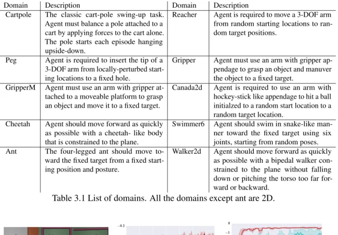
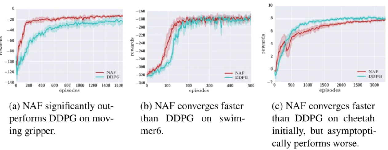
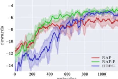
3.1 (a) Task domains: top row from left (manipulation tasks: peg, gripper, mobile gripper), bottom row from left (locomotion tasks: cheetah, swimmer6, ant). (b,c) NAF vs DDPG results on three-joint reacher and peg insertion. On reacher, the DDPG policy continuously fluctuates the tip around the target, while NAF stabilizes well at the target. . . 25 3.2 NAF vs DDPG on three domains. . . 26 3.3 NAF with exploration noise generated using the precision term (NAF-P)

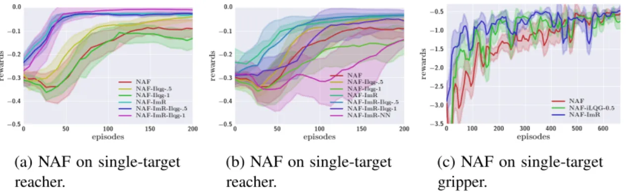
slightly outperforms the best DDPG result. Precision term is not used until step 50,000. . . 27 3.4 Results on NAF with iLQG-guided exploration and imagination rollouts (a)

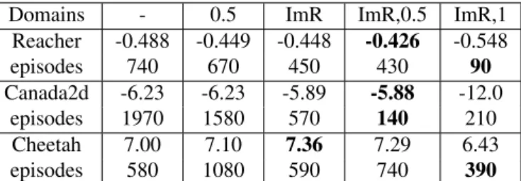
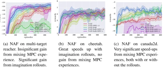
using true dynamics (b,c) using fitted dynamics. “ImR" denotes using the imagination rollout withl=10 steps on the reacher andl=5 steps on the gripper. “iLQG-x" indicates mixing x fraction of iLQG episodes. Fitted dynamics uses time-varying linear models with sample size n=5, except “-NN" which fits a neural network to global dynamics. . . 28 3.5 NAF on multi-target reacher, cheetah, and canada2d, with model-based

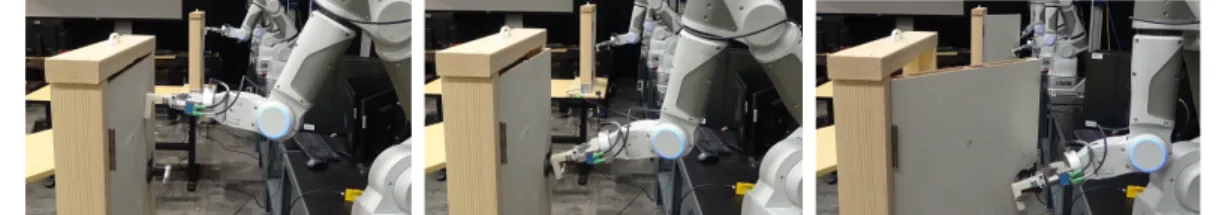
acceleration using true dynamics: “ImR" denotes using the imagination rollout,l=10 steps. “MPC-x" indicates mixingxfraction of MPC episodes. 30 3.6 Two robots learning to open doors using asynchronous NAF. The final policy

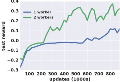
learned with two workers could achieve a 100% success rate on the task across 20 consecutive trials. . . 31 3.7 The 7-DoF arm random target reaching with asynchronous NAF on real

robots. Note that 1 worker suffers in both learning speed and final policy performance. . . 32

(18)

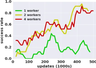
xviii List of figures 3.8 Learning curves for real-world door opening. Learning with two workers

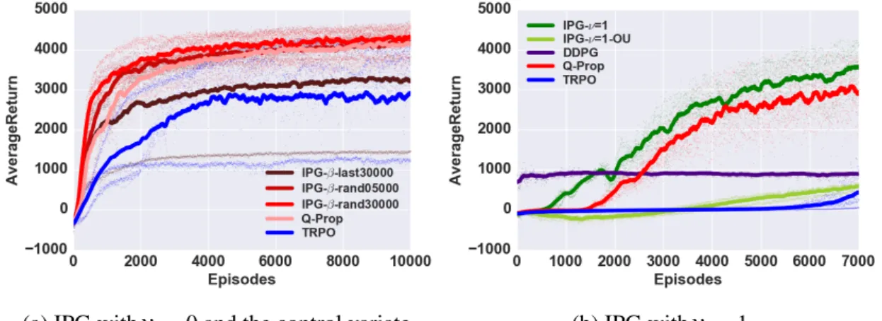
significantly outperforms the single worker, and achieves a 100% success rate in under 500,000 update steps, corresponding to about 2.5 hours of real time. . . 33 4.1 (a) IPG-ν =0 vs Q-Prop on HalfCheetah-v1, with batch size 5000. IPG-β

-rand30000, which uses 30000 random samples from the replay as samples fromβ, outperforms Q-Prop in terms of learning speed. (b) IPG-ν=1 vs other

algorithms on Ant-v1. In this domain, on-policy IPG-ν=1 with on-policy

exploration significantly outperforms DDPG and IPG-ν=1-OU, which use a

heuristic OU (Ornstein–Uhlenbeck) process noise exploration strategy, and marginally outperforms Q-Prop. . . 43 4.2 IPG-ν =0.2-π-CV vs Q-Prop and TRPO on Humanoid-v1 with batch size

10000 in the first 10000 episodes. IPG-ν=0.2-π-CV, with a small difference

ofν =0.2 multiplier, out-performs Q-Prop. All these methods have stable,

monotonic policy improvement. The experiment is cut at 10000 episodes due to heavy compute requirement of Q-Prop and IPG methods, mostly from fitting the off-policy critic. . . 46 5.1 The tasks in our experiments: (a) reaching target locations, (b) pushing a

puck to a random target, (c) training the cheetah to run at target velocities, (d) training an ant to run to a target position or a target position and velocity, and (e) reaching target locations (real-world Sawyer robot). . . 58 5.2 The comparison of TDM with the baseline methods in model-free (DDPG),

model-based, and goal-conditioned value functions (HER - Dense) on various tasks. All plots show the final distance to the goal versus 1000 environment steps (not rollouts). The bold line shows the mean across 3 random seeds, and the shaded region show one standard deviation. Our method, which uses free learning, is generally more sample-efficient than model-free alternatives including DDPG and HER and improves upon the best model-based performance. . . 59 5.3 Ablation experiments for (a) scalar vs. vectorized TDMs on 7-DoF simulated

reacher task and (b) differentτmax on pusher task. The vectorized variant per-forms substantially better, while the horizon effectively interpolates between model-based and model-free learning. . . 60

(19)

List of figures xix

B.1 TDMs with different number of updates per stepIon ant target position task. The maximum distance was set to 5 rather than 6 for this experiment, so the numbers should be lower than the ones reported in the paper. . . 84

(20)

(21)

List of tables

3.1 List of domains. All the domains except ant are 2D. . . 25 3.2 Best test rewards of DDPG and NAF policies, and the episodes it requires to

reach within 5% of the best value. “-" denotes scores by a random agent. . . 27 3.3 Best-case model-based acceleration with true dynamics models. Best test

rewards of NAF policies (first row), and the episodes it required to reach 5% of the best value (second row). “0.5" and “1" correspond to the fraction of MPC episodes. “ImR" means using imagination rollout with rollout length l=10 for reacher, canada2d, andl=5 for cheetah. . . 29 4.1 Prior policy gradient method objectives as special cases of IPG. . . 36 4.2 Comparisons on all domains with mini-batch size 10000 for Humanoid and

5000 otherwise. We compare the maximum of average test rewards in the first 10000 episodes (Humanoid requires more steps to fully converge; see the Appendix for learning curves). Results outperforming Q-Prop (or

IPG-cv-ν=0 withβ =π) are boldface. The two columns show results with on-policy

(22)

(23)

Nomenclature

Roman Symbols

a Action

p State transition probability; initial state probability pπ

t Marginal state distribution at timet for policyπ Qπ _{State-action value function (Q-function) of policy}

π

Q∗ Optimal state-action value function (optimal Q-function) R Cumulative rewards

r Reward function

s State

Vπ _{State value function of policy}_π

V∗ Optimal state value function

Greek Symbols

γ Discount factor π Policy function

ρπ γ-discounted, unnormalized state-visitation frequency of policyπ

˜

ρπ Non-discounted, unnormalized state-visitation frequency of policyπ τ Trajectory consisting of a sequence of statessand actionsa

(24)

xxiv Nomenclature AC Actor-Critic

DDPG Deep Deterministic Policy Gradient DNN Deep Neural Network

DQN Deep Q-Network ES Evolutionary Strategy

GAE Generalized Advantage Estimation IPG Interpolated Policy Gradient LSPI Least-Squares Policy Iteration LSTD Least-Squares Temporal Difference MDP Markov Decision Process

NAF Normalized Advantage Functions PG Policy Gradient

POMDP Partially-Observable Markov Decision Process PPO Proximal Policy Optimization

RL Reinforcement Learning SGD Stochastic Gradient Descent SVG Stochastic Value Gradient TD Temporal Difference

(25)

Chapter 1 Introduction

1.1 Reinforcement Learning and Sample Efficiency

We live in the world of sequential data and constant decision-making. The beauty of time, sequence, and recursion is that simple functions, e.g. laws of physics, can enable rich complex phenomena, e.g. the earth and us, to emerge as a consequence. We, and other living organisms capable of decision-making, can choose to predictively alter the course of the future by acting in the environment. This ability to achieve desired goals through interation is essential for survival as individuals or species. Richness of goals and how predictably we can accomplish them have been proposed as key metrics for defining a universal measure of intelligence (Legg and Hutter,2007;Salge et al.,2014). How we can most effectively change the passive dynamics of the world to achieve what we want, is at the core of sequential decision-making and is the fundamental problem studied in the field of reinforcement learning (RL)

Reinforcement learning (RL) studies a series of approaches for solving arbitrary goal-directed sequential decision-making problems with only high-level reward signals and no supervision. It has recently been extended to utilize large neural network policies and value functions, and has been successful in solving a range of difficult problems, such as playing computer games from pixels, the game of Go, and continuous control of humanoids in simulation (Heess et al.,2017;Lillicrap et al.,2016;Mnih et al.,2015;Schulman et al.,2016;

Silver et al.,2016). The use of deep neural networks (DNNs) to parameterize functions which are then learned from data minimizes the need for manual feature and policy engineering, and allows learning end-to-end policies mapping from high-dimensional inputs, such as images, directly to actions. However, such expressive parametrization also introduces a number of practical problems. Deep reinforcement learning algorithms tend to be sensitive to hyperparameter settings, often requiring extensive hyperparameter sweeps to find good

(26)

2 Introduction values. Poor hyperparameter settings tend to produce unstable or non-convergent learning. Deep RL algorithms also tend to exhibit high sample complexity, often to the point of being impractical to run on some real physical systems. In this thesis, we propose scalable RL methods with improved sample efficiency that connect and bridge gaps between branches of RL: model-based with model-free, and on-policy with off-policy.

1.2 Thesis Outline

• Chapter 2 provides an overview on the basics of model-based, value-based, and policy-based approaches to reinforcement learning, highlighting their differences in terms of learning signals and target functions to estimate.

• Chapter 3 discusses normalized advantage functions (NAF) and LQR-based accelera-tion of Q-learning for continuous control. The content is adapted from:

– Shixiang Gu, Timothy Lillicrap, Ilya Sutskever, Sergey Levine. “Continuous Deep Q-Learning with Model-based Acceleration”. ICML 2016. (Gu et al.,

2016b)

– Shixiang Gu*, Ethan Holly*, Timothy Lillicrap, Sergey Levine. “Deep Rein-forcement Learning for Robotic Manipulation with Asynchronous Off-Policy Updates”. ICRA 2017. (Gu et al.,2017a)

• Chapter 4 discusses interpolated policy gradient (IPG), a framework for unifying off-policy actor-critic and on-off-policy Monte Carlo off-policy gradient and providing theoretical bounds on the bias induced through imperfect critic and off-policy sampling. The content is adapted from:

– Shixiang Gu, Timothy Lillicrap, Zoubin Ghahramani, Richard E. Turner, Sergey Levine. “Q-Prop: Sample-Efficient Policy Gradient with An Off-Policy Critic”. ICLR 2017. (Gu et al.,2017b)

– Shixiang Gu, Timothy Lillicrap, Zoubin Ghahramani, Richard E. Turner, Bern-hard Schölkopf, Sergey Levine. “Interpolated Policy Gradient: Merging On-Policy and Off-On-Policy Gradient Estimation for Deep Reinforcement Learning”. (Gu et al.,2017c)

• Chapter 5 discusses temporal difference models (TDM) and shows that an off-policy value-based method with vectorized parameterization, goal-conditioned rewards, and

(27)

1.2 Thesis Outline 3

relabeling trick (Andrychowicz et al.,2017) can generalize model-based methods to achieve substantial improvements in sample efficiency. The content is adapted from:

– Vitchyr Pong*, Shixiang Gu*, Murtaza Dalal, Sergey Levine. “Temporal Differ-ence Models: Model-Free Deep RL for Model-Based Control”. ICLR 2018. (Pong et al.,2018)

Each of the papers mentioned above is through multi-author collaboration. However, in every case I was the (joint) first author. As such, I contributed the most in formulating the research, implementing the code, writing the paper, and running the experiments. I have also published the following papers whilst carrying out my PhD, but these have not been included in this thesis:

• Nilesh Tripuraneni*, Shixiang Gu*, Hong Ge, Zoubin Ghahramani. “Particle Gibbs for Infinite Hidden Markov Models”. NIPS 2015. (Tripuraneni et al.,2015)

• Shixiang Gu, Zoubin Ghahramani, Richard E. Turner. “Neural Adaptive Sequential Monte Carlo”. NIPS 2015. (Gu et al.,2015)

• Shixiang Gu, Sergey Levine, Ilya Sutskever, Andriy Mnih. “MuProp: Unbiased Backpropagation for Stochastic Neural Networks”. ICLR 2016. (Gu et al.,2016a) • Eric Jang, Shixiang Gu, Ben Poole. “Categorical Reparametrization with

Gumble-Softmax”. ICLR 2017. (Jang et al.,2017)

• Natasha Jaques, Shixiang Gu, Dzmitry Bahdanau, Jose Miguel Hernndez Lobato, Richard E. Turner, Douglas Eck. “Sequence Tutor: Conservative fine-tuning of sequence generation models with KL-control”. ICML 2017. (Jaques et al.,2017) • Benjamin Eysenbach, Shixiang Gu, Julian Ibarz, Sergey Levine. “Leave no Trace:

Learning to Reset for Safe and Autonomous Reinforcement Learning”. ICLR 2018. ( Ey-senbach et al.,2018)

• George Tucker, Surya Bhupatiraju, Shixiang Gu, Richard E. Turner, Zoubin Ghahra-mani, Sergey Levine. “The Mirage of Action-Dependent Baselines in Reinforcement Learning”. ICML 2018. (Tucker et al.,2018)

• Ofir Nachum, Shixiang Gu, Honglak Lee, Sergey Levine. “Data-Efficient Hierarchical Reinforcement Learning”. NIPS 2018. (Nachum et al.,2018)

(28)

(29)

Chapter 2 Reinforcement Learning Algorithms

This chapter provides an overview of the basic approaches in reinforcement learning. We first introduce the standard objective, functions, and mathematical notations in RL used throughout this thesis, and then move on to detail classes of RL algorithms based on two groupings: (1) model-based and model-free, and (2) on-policy and off-policy. The emphasis is put on the simplest formulations, which are often most compatible with scalable neural network function approximations. This also enables us to abstract many approaches in RL to the most basic forms, and illuminate their advantages, disadvantages and relations. Beyond the materials covered here, RL has a rich set of algorithms and theoretical analyses. We will refer readers to the excellent books bySutton and Barto(1998) andSzepesvári(2010) for more comprehensive overviews on the history and development of RL, and the survey byDeisenroth et al.(2013) for a practical understanding into challenges that arise when RL is applied to real-world applications such as robotics.

2.1 Reinforcement Learning

The basic RL formulation involves an agent interacting with a Markov Decision Pro-cess (MDP) (S,A,γ,P,r), where S denotes the fully-observed state space of the

envi-ronment and the agent, A denotes the action space, γ denotes the discount factor, P=

{p(s₀),p(s_t+1|st,at)} denotes the initial state distribution and transition dynamics of the environment, andr(s,a)denotes the reward function. At timet, an agent in states_t∈Stakes an actiona_t∈Aaccording to its policyπ(at|st), the state transitions tost+1according toP,

(30)

6 Reinforcement Learning Algorithms to maximize theγ-discounted cumulative future return,

J(π) =_E_s₀_∼_p₍_s₀₎_,_a₀_∼_π₍_a₀_|_s₀₎_,_s₁_∼_p₍_s₁_|_s₀_,_a₀₎_,_a₁_∼_π₍_a₁_|_s₁₎_,_··· " ∞

∑

t=0 γtr(st,at) # (2.1) =_Es0,a0,s1,···∼P,π " ∞

∑

t=0 γtr(st,at) # , (2.2) π∗=arg max π J(π) (2.3)

where we assume infinite planning horizon. The difficulty of RL is that we do not know the dynamicsPof the MDP and we can only sample transitions from it, usually in an episodic manner without control over initial state distributions. In certain cases, we also assume that we do not know the reward functionr(s,a)and only observe its sampled values. For real-world applications such as robotics, it is crucial to minimize the number of samples required for learning, i.e. maximize the sample efficiency of the algorithm.

The main goal is to learn the optimal policyπ∗, which can be done by directly optimizing

a parameterizedπwith respect to the above objective, known aspolicy-basedapproaches.

Alternative approaches estimate other functions from the experience data, from whichπ∗can

be efficiently derived. Two such approaches arevalue-basedandmodel-based. Value-based approaches learn the Q-functionQπ₍_s_,_a₎_{, or state-action value function, which summarizes}

the future return of taking actionafrom statesand following policyπ afterwards:

Qπ₍_s t,at) =Est+1,at+1,···∼P,π|st,at " ∞

∑

t′₌_t γt ′₋_t r(s_t′,a_t′) # . (2.4)

The estimated function can then be used to improve the policy. In particular, if the Q-function Q∗ for the optimal policy π∗ is learned, the optimal policy is directly given by π∗(at|st) =δ(at =arg maxaQ∗(st,a)).

Model-based approaches, on the other hand, estimate the dynamics ˆp(s_t+1|st,at)≈ p(s_t+1|st,at)and the reward function ˆr(s,a)≈r(s,a)through fitting approximators ˆp(st+1|st,at) and ˆr(s,a) from observed transitions {st,at,rt,st+1}, and then use the learned models to

approximately solve for the optimal policy as below,

π∗≈arg max π ˆ J(π) =arg max π Es0,a0,s1,···∼Pˆ,π " ∞

∑

t=0 γtrˆ(st,at) # . (2.5)

(31)

2.2 Model-based and Model-free Algorithms 7

Importantly, it is also trivial to use the learned model to evaluate an approximation to the state-action value function of any policyπ as,

Qπ₍_s t,at)≈Est+1,at+1,···∼Pˆ,π|st,at " ∞

∑

t′=t γt ′₋_t ˆ r(s_t′,a_t′) # . (2.6)

The quality of approximations toπ∗andQπ depends strongly on the quality of the learned

dynamics ˆPand reward function ˆr.

2.2 Model-based and Model-free Algorithms

This section describes three approaches in RL based on being model-based or model-free, where the model-free includes value-based and policy-based algorithms. For the clarify of presentation, we explicitly separate model-based from model-free in the discussion here; however, as we analyze in Chapter 5, there exists subtle connections between model-based and model-free (particularly value-based).

2.2.1 Model-based Algorithms

Model-based algorithms, more commonly known as optimal control in the control theory literatures, are a set of algorithms that utilize a learned or available approximate model of an MDP to solve for the optimal policy without relying on real environment samples. While classic control often only involves planning with an available model of the robot or the control system with minimal model learning such as online system identification, model-based algorithms in RL literatures often involve both model learning as well as model planning. A diverse set of parameterizations of the model have been explored, including locally linear dynamics as in linear-quadratic regulator (LQR) systems (Levine et al.,2016; Li and Todorov, 2004; Todorov and Li, 2005), feed-forward and recurrent neural networks (Nguyen and Widrow,1990;Schmidhuber,1990,1991;Wahlström et al.,

2015; Watter et al., 2015; Werbos,1989), and non-parametric probabilistic models such as Gaussian processes (Deisenroth and Rasmussen,2011). While subtle differences exist in their model learning objectives, simple maximium likelihood estimation (MLE) is most frequently used. Equivalently, they minimize the inclusive Kullback–Leibler (KL) divergence betweenp(s_t₊₁|st,at)and a family of variational distributionq(st+1|st,at)based on transition

(32)

8 Reinforcement Learning Algorithms samples, ˆ p=arg min q Est,at∼P,β[DKL(p(·|st,at),q(·|st,at)] (2.7) =arg max q Est,at,st+1∼P,β[logq(st+1|st,at)]. (2.8) The notation β means that that samples can come from any behavior policy and do not

need to come from on-policy rollouts based onπ. This makes the model-based approach

generally seen as anoff-policyalgorithm, capable of utilizing all samples collected during learning to make policy improvement. Furthermore, model-based RL can use the rich learning signals available in predicting high-dimensional observationst+1, e.g. an image,

which is substantially more than predicting scalar rewards or cumulative returns. These properties make model-based algorithms very sample-efficient when a good, generalizable model can be learned from samples (Deisenroth and Rasmussen,2011;Kurutach et al.,2018;

Nagabandi et al.,2017). However, when learning a good model is difficult, e.g. dynamics are discontinuous and observations are high dimensional, model-based algorithms often exhibit worse asymptotic performances (with infinite samples) than policy-based or value-based approaches that are consideredmodel-free(Gu et al.,2016b;Pong et al.,2018).

The choice of parameterization and learning objective for the model affects the model-based policy performance, but so does the choice of planning algorithm. Given a fitted model of dynamics ˆp, the derivation of the optimal policy is just another RL problem, with the following additional conditions: (1) samples can be queried infinitely, (2) states can be reset to any states during rollouts, and (3) dynamics may be differentiable. Therefore, new algorithms utilizing these additional properties, along with any standard policy-based or value-based algorithms can be used to derive the policy. In fact, recent results that have shown more success with model-based RL using neural networks have utilized dynamics-gradient-free policy derivation from the model (Ha and Schmidhuber,2018;Kurutach et al.,

2018;Nagabandi et al.,2017). Below are a list of planning algorithm examples to derive the optimal policy from a model:

1. Closed-form solve, e.g. linear-quadratic regulator (LQR), iterative LQG (iLQG) (Levine et al.,2016;Li and Todorov,2004;Todorov and Li,2005;Watter et al.,2015)

2. Gradient-based action optimization, e.g. model-predictive control (MPC) with gradient-based action updates

3. Gradient-free action optimization, e.g. MPC with gradient-free action updates ( Chebo-tar et al.,2017b;Nagabandi et al.,2017;Theodorou et al.,2010) and Monte Carlo tree search

(33)

4. Gradient-based policy optimization, e.g. PILCO (Deisenroth and Rasmussen,2011) 5. Gradient-free policy optimization, e.g. TRPO or evolutionary strategies with

model-based policy evaluation (Ha and Schmidhuber,2018;Kurutach et al.,2018) 6. Q-learning, e.g. Dyna-Q algorithms (Gu et al.,2016b;Sutton,1990)

7. Actor-critic method, e.g. stochastic value gradients (SVG) (Heess et al.,2015a) Taken together, the model parametrization, model learning objective, and planning algorithm offer a wide range of design choices for model-based algorithms. While a wide gap on asymptotic performance against model-free algorithms exists at the moment, the hope is that further research can yield substantially better results for model-based in the future.

Iterative LQG

The iterative Linear-Quadratic Gaussian (iLQG) is a popular model-based algorithm that optimizes trajectories by iteratively constructing locally optimal linear feedback controllers under a local linearization of the dynamics p(s_t+1|st,at) =N(st+1;fstst+ fatat,Ft) and a quadratic expansion of the rewardsr(st,at)(Tassa et al.,2012). Under linear dynamics and quadratic rewards, the action-value functionQ(st,at)and value functionV(st)are locally quadratic and can be computed by dynamics programming.1

Qsa,sat =rsa,sat+fsatT Vs,st+1fsat Q_sat =r_sat+f_satT V_s_,_st₊₁ Vs,st =Qs,st−QaT,stQ−1a,atQa,st

V_st =Q_st−QT_a_,_stQ−1_a_,_atQ_at Qs,sT =Vs,sT =rs,sT

(2.9)

The time-varying linear feedback controllerg(s_t) =aˆ_t+k_t+K_t(s_t−sˆ_t)maximizes the locally quadraticQ, wherek_t=−Q−1_a_,_atQ_at,K_t =−Q−1_a_,_atQ_a,st, and ˆst,aˆt denote states and actions of the current trajectory around which the partial derivatives are computed. Employing the max-imum entropy objective (Levine and Koltun,2013), we can also construct a linear-Gaussian controller, wherecis a scalar to adjust for arbitrary scaling of the reward magnitudes,

π_tiLQG(at|st) =N(at; ˆat+kt+Kt(st−sˆt),−cQ−1a,at) (2.10)

1_{While standard iLQG notation denotes}_Q_,_V_{as discounted sum of costs, we denote them as sum of rewards}

(34)

10 Reinforcement Learning Algorithms When the dynamics are not known, a particularly effective way to use iLQG is to combine it with learned time-varying linear models ˆp(st+1|st,at). In this variant of the algorithm, trajectories are sampled from the controller in Eq. 2.10 and used to fit time-varying linear dynamics with linear regression. These dynamics are then used with iLQG to obtain a new controller, typically using a KL-divergence constraint to enforce a trust region, so that the new controller does not deviate too much from the region in which the samples were generated (Levine and Abbeel,2014).

2.2.2 Value-based Algorithms

Value-based approaches are model-free algorithms that estimate value functionV(s)or state-action value functionQ(s,a)in order to efficiently solve for the optimal policy. The core of most value-based approaches is to find functions that satisfy Bellman equations, i.e. their recursive dynamic programming definitions. While value-based algorithms are very broad in scope (Sutton and Barto,1998;Szepesvári,2010), we will focus on methods that estimate Qπ _or_Q∗_{, since these are methods that can directly utilize off-policy samples for learning.}

Specifically, we can re-writeQπ _{definition in Eq. 2.4 recursively as,}

Qπ₍_s t,at) =Est+1,at+1,···∼P,π|st,at " ∞

∑

t′=t γt ′₋_t r(s_t′,a_t′) # (2.11) =r(s_t,a_t) +γ_E_s_t₊₁_∼_p_(·|_s_t_,_a_t₎_,_a_t₊₁_∼_π_(·|_s_t₊₁₎[Qπ(st+1,at+1)]. (2.12)

This suggests minimizing the following surrogate objective for learning a parameterized state-action value functionQwto approximateQπ,

L(w) =_E_s_t_,_a_t_,_s_t₊₁_∼_P_,_β h (Q_w(s_t,a_t)−y_t)2 i (2.13) y_t=r(s_t,a_t) +γ_E_a_t₊₁_∼_π_(·|_s_t₊₁)[Qw(st+1,at+1)]. (2.14)

Such method that optimizes for Bellman consistency is also known as temporal difference (TD) learning (Tesauro,1995), a method for approximate dynamic programming. In this example, it is evaluatingQπ_{, i.e. performing policy evaluation; however, a different Bellman}

equation forQ∗ leads to the renowned Q-learning algorithm (Watkins and Dayan,1992). Notice that for these temporal difference learning objectives, we could directly use samples from any behavior policyβ as similarly done in the model-based objective of Eq. 2.8. The

capability for simple off-policy learning enable value-based methods to be more sample efficient than policy-based approaches which are generally only effective on-policy; however, since it optimizes for a surrogate Bellman error objective, its convergence is harder to

(35)

analyze and guarantee, particularly with nonlinear function approximation and off-policy sampling (Bhatnagar et al., 2009; Sutton et al., 2009a,b; Tsitsiklis and Van Roy, 1996;

Watkins and Dayan,1992). With the mainstream application of neural network function approximations in value-based approaches (Gu et al.,2016b;Lillicrap et al.,2016;Mnih et al.,

2015), a series of techniques have been introduced to combat such instability, such as replay buffer (Lin,1992;Mnih et al.,2015;Schaul et al.,2015b), exploration heuristics (Gal and Ghahramani,2016;Osband et al.,2016), target networks (Lillicrap et al.,2016;Mnih et al.,

2015), advantage-value decomposition (Gu et al.,2016b;Wang et al.,2016), conservative target value estimators (Fujimoto et al.,2018;Hasselt,2010;Van Hasselt et al.,2015), mixing multi-step returns (Munos et al.,2016), and soft value iteration (Haarnoja et al.,2017;Rawlik et al.,2013). We will not go through these details and instead focus on their basic forms to highlight how they relate to model-based and policy-based in later sections.

Q-Learning

Q-learning (Watkins and Dayan,1992) is one of the most popular value-based algorithms and makes use of the Bellman optimality equation defined forQ∗,

Q∗(s_t,a_t) =_E_s_t₊₁_,_a_t₊₁_,_···∼_P_,_π∗_|_s t,at " ∞

∑

t′₌_t γt ′₋_t r(s_t′,a_t′) # (2.15) =r(s_t,a_t) +γ_E_s_t₊₁_∼_p_(·|_s_t_,_a_t₎ h max a Q ∗₍_s t+1,a) i . (2.16)

A practical implementation for deep learning optimizes a parameterized Q-functionQw, a deep Q-network (DQN) (Mnih et al.,2015), using stochastic gradient descent (SGD) on the following objective, L(w) =_E_s_t_,_a_t_,_s_t₊₁_∼_P_,_βh(Q_w(s_t,a_t)−y_t)2i (2.17) y_t =r(s_t,a_t) +γmax a Q ′₍_s t+1,a), (2.18)

whereQ′ denotes the target network which syncs with the mainQ_w at some fixed inter-vals (Mnih et al.,2015) or smoothly tracksQ_w(Lillicrap et al.,2016). β represents sampling

from replay buffer (Lin,1992;Mnih et al.,2015), whose policy is effectively a mixture of all exploration policies, which usually adapt with changingQ_w. As noted in Section 2.2.2, many techniques have been devised to stablize Q-learning with neural network function approximations.

For discrete action spaces, Eq. 2.17 can be optimized straightforwardly; however, for continuous action space, the maxa operator makes the target value computation difficult.

(36)

12 Reinforcement Learning Algorithms Actor-critic methods (Sutton et al., 1999a) are thus typically proposed for value-based approaches in continuous action spaces. In Chapter 3, we discuss how deep Q-learning can be directly extended to continuous action space by adopting a specific parameterization of Q-functions.

2.2.3 Policy-based Algorithms

Policy-based (PG) approaches, and in particular policy gradient methods, are model-free algorithms and considered the most direct way to find the optimal policy, since they do not involve surrogate objectives as in model-based or value-based approaches. They directly apply gradient ascent with respect to the RL objectiveJ(π)in Eq. 2.2. Specifically, for a

parameterized stochastic policyπθ, the gradient ofJ(π) =J(θ)with respect toθ is given

by the following, where τt+1={st+1:∞,at+1:∞} denotes a partial trajectory of states and actions, ˆQ(s_t,a_t,τt+1) =∑∞_t′₌_tγt

′₋_t

r(s_t′,a_t′)denotesγ-discounted cumulative rewards,pπ_t(st) is the marginal state distribution at timet for policyπ, andρπ(s) =∑∞_t₌₀γtpπ_t(st=s)is the unnormalizedγ-discounted state visitation frequency,

∇θJ(θ) =∇θEs0,a0,s1,···∼P,πθ " ∞

∑

t=0 γtr(st,at) # (2.19) =_Es0,a0,s1,···∼P,πθ " ∞

∑

t=0 ∇_θlogπ_θ(at|st) ! ∞

∑

t=0 γtr(st,at) !# (2.20) =_Es0,a0,s1,···∼P,πθ " ∞

∑

t=0 ∇θlogπθ(at|st) ∞

∑

t′₌_t γt ′ r(s_t′,a_t′) !# (2.21) =_E_s₀,a0,s1,···∼P,πθ " ∞

∑

t=0 ∇θlogπθ(at|st)γtQˆ(st,at,τt+1) # (2.22) = ∞

∑

The last line of derivation is based on the definition ofQπ_{. A subtle detail to note is that in}

practical algorithms, we do not use state samplessfromρπ(s), but instead use normalized

undiscounted state visitation frequency ¯ρπ(s)∝ ∑∞_t=0ptπ(st =s).Thomas(2014) discusses that this induces bias in the gradient estimation; however, this bias is essential for good,

(37)

2.3 On-Policy and Off-Policy Algorithms 13

practical performance. In the rest of this thesis, we only discuss additional biases on top of the practical implementation bias, and also interchangeably use these two definitions of state visitation distribution withρπ. Note that to make the original discounted definition ofρπ

normalized, we simply multiply by 1−γ.

2.3 On-Policy and Off-Policy Algorithms

An RL algorithm is consideredon-policyif it mainly uses transition samples from the current policy π to improve the policy at each iteration. By contrast, anoff-policyalgorithm can

reuse samples from any policy (past policies or arbitrary behavior policies) to make effective policy improvements on the same batch of data. In this section, we use the policy gradient derivation in Section 2.2.3 as a starting point and introduce its on-policy and off-policy variants.

2.3.1 On-Policy Likelihood Ratio Policy Gradient

Policy gradients derived in Eq. 2.19 are on-policy, since their estimations involve expectation over transitions from policy π. In particular, we call the gradient estimator in Eq. 2.24

Monte Carlo policy gradient estimatororlikelihood ratio policy gradient estimator, since it relies on Monte Carlo estimate of the Q-function ˆQ(s,a,τ)and a likelihood ratio or score

function gradient estimator. It is the basis of popular on-policy policy gradient algorithms such as REINFORCE (Williams,1992), trust-region policy optimization (TRPO) (Schulman et al., 2015a), asynchronous advantage actor-critic (A3C) (Mnih et al.,2016), proximal policy optimization (PPO) (Schulman et al.,2017). In practice, a number of techniques are required to make this estimator lower variance, such as baselines (Weaver and Tao,

2001;Williams,1992) and generalized advantage estimation (Schulman et al.,2016). State-dependent baselines (Mnih and Gregor,2014;Schulman et al.,2015a;Williams,1992) are particularly appealing since they do not introduce bias (Williams,1992) and can be trained easily with neural function approximation. Specifically, the state-dependent baseline is applied as, ∇θJ(θ) =Est∼ρπ_(·)_,_a_t_∼_π θ(·|st),τt+1∼P,πθ|st,at ∇θlogπθ(at|st) Qˆ(st,at,τt+1)−Vφ(st) , (2.27) whereV_φ is learned to approximateVπ_{. Empirically, this simple unbiased technique leads to}

substantial variance reduction (Tucker et al.,2018;Weaver and Tao,2001;Williams,1992). WhileVπ _{is not the baseline that can optimally reduce the variance (}_{Weaver and Tao}_,₂₀₀₁_),

(38)

14 Reinforcement Learning Algorithms its estimation is generally simpler and is a preferred choice in practical Monte Carlo policy gradient algorithms (Mnih et al.,2016;Schulman et al.,2015a,2017).

The most appealing aspect of on-policy Monte Carlo policy gradient methods is their simplicity and stability. Because they do not rely on surrogate objectives as optimized in value-based or model-based approaches and use unbiased Monte Carlo estimate ˆQ(s,a,τ),

their convergence properties are easier to analyze and optimization algorithms with provable policy improvement guarantees have been devised (Gu et al.,2017c;Kakade,2001;Schulman et al.,2015a). The high-variance nature of the Monte Carlo estimation can be alleviated by taking large batch of samples per policy gradient update, or trading it off with slight bias in gradient estimation that usually does not cause performance degradation in practice (Gu et al.,2017c;Mnih et al.,2016;Schulman et al.,2016). The downside of these Monte Carlo methods is that they often cannot utilize off-policy samples effectively without introducing non-trivial bias, since naíve importance correction does not scale well with action and temporal dimensions (Levine and Koltun,2013;Thomas and Brunskill,2016). This makes the Monte Carlo policy gradient algorithms very data intensive. However, these algorithms directly learnπ∗and the approximation ofVπ is only used for variance reduction, so they

can generally use much simpler function approximations, such as smaller neural networks or linear function approximation, than in value-based or model-based approaches (Duan et al.,

2016;Gu et al.,2017c;Lillicrap et al.,2016;Rajeswaran et al.,2017). Such simplicity may sometimes make Monte Carlo policy gradient still a preferred method of choice.

2.3.2 Off-Policy Expected Actor-Critic

To arrive at an off-policy policy gradient algorithm, we again start from the derivation in Eq. 2.19. In contrast to Eq. 2.24, we call the gradient estimator in Eq. 2.26deterministic policy gradient estimator(Gu et al.,2017b,c),expected policy gradient estimator (Asadi et al.,2017;Ciosek and Whiteson,2018;Degris et al.,2012), orall-action policy gradient estimator(Sutton,2000), since it uses a criticQπ₍_s_,_a₎_{to compute analytic gradient integrated}

over immediate actiona. Importantly, the criticQπ_{can be estimated using off-policy temporal}

difference learning. Such off-policy policy evaluation provides the foundation for deriving off-policy actor-critic algorithms.

Actor-critic methods (Sutton et al., 1999a) optimize a value function Qπ _or _Vπ_{, the}

critic, and a policy functionπ, the actor, iteratively. They are model-free methods and

considered an hybrid approach between value-based and policy-based. The core of the idea is captured in policy iteration algorithm (Howard,1964), which uses policy evaluation to estimateQπ _or_Vπ _{and uses policy improvement to improve the policy}_π _{locally with respect}

(39)

2.3 On-Policy and Off-Policy Algorithms 15

updates, such as least-squares policy iteration (LSPI) (Lagoudakis and Parr,2003;Lagoudakis et al.,2002), which iterates between least-squares temporal difference (LSTD) (Bradtke and Barto,1996) solve of Qπn₍_s_,_a₎_{given policy}_πn _{at iteration}_{n, and analytic update of} the actorπn+1(a|s) =δ(a=arg max_a′Qπ

n

(s,a′)). Similarly, with neural network function approximations, the algorithm alternates between the following two minimization objectives with respect toQwand a parameterized policyπθ,

L(w) =_E_s_t_,_a_t_,_s_t₊₁_∼_P_,_β h (Q_w(s_t,a_t)−y_t)2 i (2.28) y_t=r(s_t,a_t) +γ_E_a_∼_π θ(·|st+1)Q ′₍_s t+1,a) (2.29) L(θ) =−_E_s_t_∼_P_,_β_E_a_t_∼_π θ(·|st)Qw(st,at) (2.30) Since optimizing each objective is expensive, practical algorithms often perform a small number of SGD updates per objective for iteratively learningQ_w andπθ. In the limiting case

with a deterministic policyπθ(a|s) =δ(a=µθ(s)), we get deterministic policy gradient

(DPG) algorithm (Lever,2014;Lillicrap et al.,2016). If we use a stochastic policy (Gu et al.,

2017c;Haarnoja et al.,2018;Heess et al.,2015a), the gradient for the negative policy loss is given below, where we useρβ to denote state visitation frequency under policyβ,

−∇_θL(θ) =_E_s t∼ρβ ∇_θ_E_a_t_∼_π θ(·|st)Qw(st,at) (2.31) =_E_s t∼ρβ_(·)_,_a_t_∼_π θ(·|st)[∇θlogπθ(at|st)Qw(st,at)]. (2.32)

The second line is unnecessary in most cases, since if the action is discrete, analytic integra-tion with respect to acintegra-tion is usually tractable, and if the acintegra-tion is continuous and the policy a simple distribution such as Gaussian, reparameterization trick (Kingma and Welling,2014) can be used to compute a lower variance estimator. However, we explicit write this using the score function estimator form to illuminate the closeness of actor-critic gradient with Monte Carlo policy gradient in the next section.

As we contrast Eq. 2.26 with Eq. 2.31, we observe that the biases in off-policy actor-critic gradient only come from two sources: approximation ofQπ _through_Q

w and off-policy state sampling using ρβ instead of ρπ. In Chapter 4, we show that we can derive theoretical

bounds on policy gradient biases in actor-critic methods based on those two factors, and empirically demonstrate that by changing design choices in off-policy actor-critic algorithms, we can better model the stable learning behavior of on-policy Monte Carlo policy gradient algorithms with significantly improved sample efficiency.

An intriguing property of such stochastic gradient actor-critic algorithm is that by simply changing the SGD update ratio of the two objectives, it can interpolate between Q-learning

(40)

16 Reinforcement Learning Algorithms and policy gradient, discussed in Section 2.2.2 and Chapter 2.2.3 respectively. Specifi-cally, if we have many actor updates per critic update, the actor is effectively amortizing arg maxaQπ(s,a)at each iteration and the learning dynamics is similar to that of Q-learning. If we have many critic updates per actor update, the critic is doing full policy evaluation to estimateQπ_{, and the actor is updated using a gradient estimate resembling that of classic}

policy gradient. We will discuss such connection more in the next chapter on policy gradient. In practice, these algorithms often use simple one-to-one update ratio (Lillicrap et al.,2016), making the analysis of learning dynamics difficult. In Chapter 4, we discuss how a variant of our interpolated policy gradient (IPG) algorithm, which does 1-to-5000 actor-to-critic up-dates, performs much more stably than prior methods, possibly due to its closer resemblance to the stable policy gradient algorithm.

(41)

Chapter 3 Continuous Deep Q-Learning with

Model-based Acceleration

In this chapter, we derive a variant of Q-learning (Watkins and Dayan,1992) that can be used in continuous domains. Model-free reinforcement learning in domains with continuous actions is typically handled with policy search methods (Peters et al.,2010;Peters and Schaal,

2006). Integrating value function estimation into these techniques results in actor-critic algorithms (Hafner and Riedmiller,2011; Lillicrap et al.,2016; Schulman et al.,2015a), which combine the benefits of policy search and value function estimation, but at the cost of training two separate function approximators with respect to different optimization objectives. Our proposed Q-learning algorithm for continuous domains, which we call normalized advantage functions (NAF), avoids the need for a second actor or policy function, resulting in a simpler algorithm. The simpler optimization objective and the choice of value function parameterization result in an algorithm that is substantially more sample-efficient when used with large neural network function approximators on a range of continuous control domains.

Beyond deriving an improved model-free deep reinforcement learning algorithm, we also seek to incorporate elements of model-based RL to accelerate learning, without giving up the strengths of model-free methods. One approach is for off-policy algorithms such as Q-learning to incorporate off-policy experience produced by a model-based planner. However, while this solution is a natural one, our empirical evaluation shows that it is ineffective at accelerating learning. As we discuss in our evaluation, this is due in part to the nature of value function estimation algorithms, which must experience both good and bad state transitions to accurately model the value function landscape. We propose an alternative approach to incorporating learned models into our continuous-action Q-learning algorithm based on imagination rollouts: on-policy samples generated under the learned model, analogous to the Dyna-Q method (Sutton,1990). We show that this is extremely effective when the learned

(42)

18 Continuous Deep Q-Learning with Model-based Acceleration dynamics model perfectly matches the true one, but degrades dramatically with imperfect learned models. However, we demonstrate that iteratively fitting local linear models (Li and Todorov,2004) to the latest batch of on-policy or off-policy rollouts provides sufficientlocal accuracy to achieve substantial improvement using short imagination rollouts in the vicinity of the real-world samples.

Lastly, we include a demonstration of an asynchronous variant of our NAF algorithm running across a cluster of robots. We demonstrate that, contrary to commonly held assump-tions about sample inefficiency of model-free algorithms, off-policy deep Q-function based algorithms such as NAF can achieve training times that are suitable for real robotic systems. Our real world experiments show that our approach can be used to learn a door opening skill from scratch under 2.5 hours with 2 robot arms, using only general-purpose neural network representations and without any human demonstrations. To the best of our knowledge, this is the first demonstration of autonomous door opening that does not use human-provided examples for initialization.

3.1 Normalized Advantage Functions

Q-learning (Watkins and Dayan, 1992) requires evaluating arg maxaQ(s,a) in order to compute the update target and derive the optimal policy, as shown in Eq. 3.1. When action ais continuous andQis a complex function approximation such as a neural network, this optimization is generally expensive or intractable. A naïve approach to get around this problem is to discretize the continuous action space; however, this approach scales poorly with the action dimension since usingBbins per dimension forN-dimensional action space createsBN discrete actions (Lillicrap et al.,2016).

min θ Est,at,st+1∼β [(Q_θ(s_t,a_t)−y_t)2], y_t =r_t+γmax a Q ′₍_s t+1,a) (3.1) µθ(st) =arg max a Qθ(st,a) (3.2)

We propose a simple method to enable Q-learning in continuous action spaces with deep neural networks, which we refer to as normalized advantage functions (NAF). The idea behind normalized advantage functions is to represent the Q-functionQ(s_t,a_t)in Q-learning in such a way that its maximum with respect to a_t, arg maxatQ(st,at), can be determined

easily and analytically during the Q-learning update. While a number of representations are possible that allow for analytic maximization, the one we use in our implementation is based on a neural network that separately outputs a value function termV(s)and an advantage term

(43)

3.1 Normalized Advantage Functions 19

P(s|θP) is a state-dependent, positive-definite square matrix, which is parametrized by

P(s|θP) =L(s|θP)L(s|θP)T, whereL(s|θP)is a lower-triangular matrix whose entries come

from a linear output layer of a neural network, with the diagonal terms exponentiated. While this representation is more restrictive than a general neural network function, since the Q-function is quadratic in a, the action that maximizes the Q-function is always given by

µ(s|θµ). We use this representation with a deep Q-learning algorithm analogous toMnih et al.(2015), using target networks and a replay buffers as described byLillicrap et al.(2016). NAF, given by Algorithm 1, is considerably simpler than DDPG.

Algorithm 1Continuous Q-Learning with NAF

Randomly initialize normalized Q networkQ(s,a|θQ).

Initialize target networkQ′with weightθQ′←θQ.

Initialize replay bufferR← /0.

forepisode=1,Mdo

Initialize a random processNfor action exploration Receive initial observation states₁∼p(s₁)

fort=1,T do

Select actiona_t=µ(st|θµ) +Nt Executea_t and observer_t ands_t+1

Store transition (st,at,rt,st+1) inR

foriteration=1,Ido

Sample a random minibatch ofmtransitions fromR Setyi=ri+γV′(si+1|θQ

′ )

UpdateθQby minimizing the loss: L= _N1∑i(yi−Q(si,ai|θQ))2 Update the target network: θQ′←τ θQ+ (1−τ)θQ′

end for end for end for

Decomposing Q into an advantage term A and a state-value term V was suggested by Baird III (1993); Harmon and Baird III (1996), and was recently explored by Wang et al.(2016) for discrete action problems. Normalized action-value functions have also been proposed byRawlik et al.(2013) in the context of an alternative temporal difference learning algorithm. However, our method is the first to combine such representations with deep neural networks into an algorithm that can be used to learn policies for a range of challenging

(44)

20 Continuous Deep Q-Learning with Model-based Acceleration continuous control tasks. In general,Adoes not need to be quadratic, and exploring other parametric forms such as multimodal distributions is an interesting avenue for future work.

3.1.1 Locally-Invariant Exploration for Normalized Advantage

Func-tions

Exploration is an essential component of reinforcement learning algorithms. The simplest and most common type of exploration involves randomizing the actions according to some distribution, either by taking random actions with some probability (Mnih et al., 2015), or adding Gaussian noise in continuous action spaces (Schulman et al.,2015a). However, choosing the magnitude of the random exploration noise can be difficult, particularly in high-dimensional domains where different action dimensions require very different exploration scales. Furthermore, independent (spherical) Gaussian noise may be inappropriate for tasks where the optimal behavior requires correlation between action dimensions, as for example in the case of the swimming snake described in our experiments, which must coordinate the motion of different body joints to produce a synchronized undulating gait.

The NAF provides us with a simple and natural avenue to obtain an adaptive exploration strategy, analogously to Boltzmann exploration. The idea is to use the matrix in the quadratic component of the advantage function as the precision for a Gaussian action distribution. This naturally causes the policy to become more deterministic along directions where the advantage function varies steeply, and more random along directions where it is flat (Ciosek and Whiteson,2018;Haarnoja et al.,2017;Heess et al.,2012). The corresponding policy is given by π(a|s) =expQ(s,a|θ Q₎ / Z expQ(s,a|θQ)_da =N(µ(s|θµ),cP(s|θP)−1). (3.4)

Previous work also noted that generating Gaussian exploration noise independently for each time step was not well-suited for many continuous control tasks, particularly simulated robotic tasks where the actions correspond to torques or velocities (Lillicrap et al.,2016). The intuition is that, as the length of the time-step decreases, temporally independent Gaussian exploration will cancel out between time steps. Instead, prior work proposed to sample noise from an Ornstein-Uhlenbech (OU) process to generate a temporally correlated noise sequence (Lillicrap et al.,2016). We adopt the same approach in our work, but sample the innovations for the OU process from the Gaussian distribution in Equation 3.4. Lastly, we note that the overall scale ofP(s|θP)could vary significantly through the learning, and depends on the

(45)

3.2 Accelerating Model-free Learning with Model-based Rollouts 21

magnitude of the cost, which introduces an undesirable additional degree of freedom. We therefore use a heuristic adaptive-scaling trick to stabilize the noise magnitudes.

3.2 Accelerating Model-free Learning with Model-based

Rollouts

While NAF provides some advantages over actor-critic model-free RL methods in contin-uous domains, we can improve their data efficiency substantially under some additional assumptions by exploiting learned models. We will show that incorporating a particular type of learned model into Q-learning with NAFs significantly improves sample efficiency, while still allowing the final policy to be finetuned with model-free learning to achieve good performance without the limitations of imperfect models.

3.2.1 Model-Guided Exploration

One natural approach to incorporating a learned model into an off-policy algorithm such as Q-learning is to use the learned model to generate good exploratory behaviors using planning or trajectory optimization. To evaluate this idea, we utilize the iLQG algorithm (Tassa et al.,

2012) to generate good trajectories under the model, and then mix these trajectories together with on-policy experience by appending them to the replay buffer. Note that all experiences are still collected from the real environment, except the exploration policy includes an iLQG component from model-based planning. Interestingly, we show in our evaluation that, even when such exploration policy is close to optimal, e.g. planning under the perfect model, the improvement obtained from this approach is often quite small, and varies significantly across domains and choices of exploration noise. The intuition behind this result is that off-policy iLQG exploration is too different from the learned policy, and Q-learning must consider alternatives in order to ascertain the optimality of a given action. That is, it’s not enough to simply show the algorithmgoodactions, it must also experience bad actions to understand which actions are better and which are worse.

3.2.2 Imagination Rollouts

As discussed in the previous section, incorporating off-policy exploration from good, narrow distributions, such as those induced by iLQG, often does not result in significant improvement for Q-learning. These results suggest that Q-learning, which learns a policy based on minimizing temporal differences, inherently requires noisy on-policy actions to succeed. In

Sample-Efficient Deep Reinforcement Learning for Continuous Control