Yours, Mine and Ours:
Do Divorce Laws Affect the Intertemporal
Behavior of Married Couples?
∗
Alessandra Voena
February 2013
Abstract
This paper examines how divorce laws affect couples’ intertemporal choices and wellbeing. Exploiting panel variation in U.S. laws, I estimate the parameters of a model of household decision making. Household survey data indicate that the introduction of unilateral divorce in states that imposed an equal division of property is associated with higher household savings and lower female employment, implying a distortion in household assets accumula-tion and a transfer towards wives whose share in household resources is smaller than their husband’s share. When spouses share consumption equally, separate property or prenuptial agreements can reduce distortions and increase equity.
∗Department of Economics, The University of Chicago. Email: [email protected]. I thank my adviser Luigi Pistaferri and Mich`ele Tertilt as well as Caroline Hoxby, Petra Moser and Monika Piazzesi for their outstanding guidance as part of my dissertation committee at Stanford University. I am also grateful to Ran Abramitzky, Stefania Albanesi, Rick Banks, Maristella Botticini, Giacomo De Giorgi, Paula England, Max Floetotto, Seema Jayachandran, Hamish Low, Aprajit Mahajan, Neale Mahoney, Ellen McGrattan, Costas Meghir, Andrea Pozzi, Victor Rios-Rull, Martin Schneider, Brett Turner as well as participants in seminars and conferences. I owe special thanks to Elizabeth Powers and Jeffrey Gray, who provided critical data. I acknowledge the financial support of the Leonard W. Ely & Shirley R. Ely Graduate Student Fellowship through a grant to SIEPR and the Michelle R. Clayman Institute for Gender Studies Graduate Dissertation Fellowship while a PhD student at Stanford University.
This paper examines how property rights within marriage regulated by divorce laws influence the intertemporal behavior and the wellbeing of married people. During the 1970s and 1980s, most U.S. couples entered a legal system in which each spouse can obtain divorce without the consent of the other spouse and keep a fraction of the marital assets, independently of who holds the formal title to the property (Golden 1983). This study explores the impact of the introduction of this regime, namely of unilateral divorce and of equitable distribution, on the intertemporal behavior of couples. It also analyzes how the current divorce legal system affects the wellbeing of married and divorced women, who are often believed to face more negative consequences of divorce compared to men (e.g. Weitzman 1985 and 1996, Peterson 1996).
To understand the welfare implications of divorce law reforms, I build a dynamic model of household decision making that captures the key aspects of these laws. The model suggests that the impact of divorce laws crucially depends on how spouses allocate resources (consumption, leisure, assets) while married: only a spouse who has a sufficiently lower share of marital resources compared to the other spouse benefits from an equal division of property upon divorce, especially if (s)he can obtain divorce without the consent of the other spouse.
To uncover the parameters of intra-household allocation of resources, I examine the changes in household savings and wives’ employment status in response to the reforms in U.S. divorce laws. In particular, I exploit the variation in U.S. divorce laws over time and across states using data from the Panel Study of Income Dynamics and from the National Longitudinal Survey of Young and Mature Women, examining the behavior of the couples marriedbefore such reforms. These samples span from the late 1960s to the 1990s. Two main facts emerge from these surveys. First, the introduction of unilateral divorce in states where property is divided equally leads to a significantly higher accumulation of assets compared to states where property is not divided by the courts, but rather assigned to the spouse who holds the title to the property. Second, when unilateral divorce is introduced in states where property is divided equally, married women become less likely to work, while no change is observed in states that do not impose an equal division of property.
These estimates provide information to identify for the parameters of intra-household allo-cation in the dynamic model and they are consistent with the prediction that unilateral divorce results in limited commitment within marriage and in a reallocation of resources inside the
house-hold. Property division laws affect each spouse’s divorce allocation. When a spouse can divorce unilaterally, the divorce allocations affect the intra-household allocations during marriage. This channel does not operate when divorcing requires the consent of both spouses. I use the estimated structural parameters to compute the welfare effects of the reforms and to perform counterfactual experiments, which examine who benefits and who loses from alternative legal regimes and from prenuptial agreements.
The dynamic model, estimated by indirect inference, replicates the responses of assets accu-mulation and female employment when the wife’s share of household resources in marriage before the reforms is sufficiently low compared to her husband’s share, i.e. if wives’ Pareto weight in the household planning problem is lower than their husband’s Pareto weight. In particular, for couples married before the reforms, I estimate wives’ Pareto weight to be equal to a third of their husband’s Pareto weight. When mutual consent divorce is in place, such weights entirely determine the ratio of the marginal utilities of spouses’ consumption. After unilateral divorce is introduced, that ratio may change to make it incentive-compatible for spouses to remain married. Women in the sample benefit from the laws that impose an equal division of property upon divorce, because they have a lower share of the couples’ resources (including assets) compared to their husband. My simulation suggests that these women would obtain a larger share of household assets at the time of divorce in community property states (where assets are divided equally) than in a title-based states (where assets are assigned to the spouse who holds the title to the property, reflecting the intra-household allocations). Equal division of property alters the allocation of resources in divorce compared the intra-household allocation, and unilateral divorce leads the divorce allocation to influence the intra-household one.
The model indicates that asset accumulation during marriage increases because spouses’ individual incentives to save are distorted by the reforms. Because mandated equal division of property does not reflect the allocation of resources within marriage, such regime results in the equivalent of a tax on savings for the spouse with larger Pareto weight, and a subsidy for the other spouse. For sufficiently low values in the wives’ Pareto weight, the model also replicates the decline in female employment that follows the reforms. Unilateral divorce allows women who live in community property states to credibly exercise the threat of divorce and to gain, on average, more consumption and leisure also during marriage compared to the allocation in mutual
consent divorce. Hence, a more symmetric distribution of consumption in marriage follows from the symmetric distribution of resources in divorce that the equal division of property imposes.
I use the estimates of the parameters of the dynamic model to examine the welfare implications of the current property division rules. Given the estimates of the intra-household allocation parameters, my simulations suggest that, as intended by the policymakers who promoted it, the equal division of property granted more assets to women in the 1970s and ’80s compared to a system based on who owns the formal title to the property. While such system benefits women with a low share in household resources, it may prevent women whose Pareto weight is close to their husband’s weight from smoothing the marginal utility of their consumption upon divorce. When women consume as much as their husband in marriage, but have lower permanent income (for example, because of a gender wage gap), they may be better off in a separate property regime or with prenuptial agreements, as they may need to accumulate more savings to smooth the marginal utility of their consumption in case of divorce. Community property may preclude women from doing so, leaving them even more exposed to the costs of marital disruption. At the same time, community property distorts the intertemporal behavior of the couples and, from the point of view of the household, may provide lower utility than separate property. My counterfactual experiments indicate that reverting to separate property or promoting prenuptial agreements may lead increase the wellbeing of secondary earners at divorce, while reducing the distortions in the intertemporal choices of couples.
The contribution of this paper is threefold. First, I develop and estimate a dynamic model that explicitly incorporates mutual consent versus unilateral divorce regimes and property division laws. In a dynamic setting, the introduction of unilateral divorce results in limited commitment to intra-household allocation, which is not present in the mutual consent regime. Intra-household reallocation in favor of wives, due to limited commitment, provides a straightforward explanation for the reduction in their likelihood of employment that is observed in survey data when unilateral divorce is introduced in community property states. This finding supports the evidence on the presence of inefficiencies (Udry 1996) and, in particular, of limited commitment (Mazzocco 2007, Mazzocco et al. 2009) in intra-household decision making.
Second, this paper documents and explains the empirical relationship between changes in divorce laws (unilateral divorce and property division rules) and the saving behavior of married
couples, adding to the literature that examines how unilateral divorce affects household out-comes, such as labor supply (Gray 1998, Stevenson 2008), the welfare of children (Gruber 2004), the divorce rate (Friedberg 1998, Wolfers 2006), household specialization (Stevenson 2007) and domestic violence (Stevenson and Wolfers 2006). In addition to the unilateral divorce reform, I document and exploit the variation in the introduction of equitable distribution over the course of the 1970s and 1980s. To isolate such a relationship from selection and sorting issues, I ex-amine a sample of couples that married before these reforms. Using panel household data, I show that asset accumulation and female employment respond to divorce law reforms in a way that is consistent with the predictions of the model. Understanding why the divorce laws affect the incentives to save and invest may have important policy implications, given the frequency of divorce in the United States and the fact that divorce laws are subject to continuous changes through the actions of courts and lawmakers.For example, in the summer of 2010, the state of New York approved no-fault unilateral divorce. Other states have introduced or consider in-troducing covenant marriages, which require the consent of both spouses to be broken.1 Little
is known about how or why the intertemporal behavior during marriage may respond to such reforms. Today, judges, legal authors and lawyers primarily rely on anecdotal evidence and personal experience when evaluating property division (Turner, 2005).
Third, this study illustrates the implications of the current U.S. property division laws on cou-ples’ welfare and shows that the equal division of property can sometimes result in the opposite of what policymakers intended when they promoted the removal of separate property. Divorce can generate significant economic costs, such as direct legal and relocation costs, as well as loss of economies of scale and risk sharing. It can be especially costly for the spouse with lower perma-nent income, who can no longer benefit from sharing resources with the partner. Because there is no market insurance for divorce, self-insurance plays a central role in consumption smoothing. This paper investigates how different ways of dividing property at the time of divorce can affect the ability of secondary earners to use savings to smooth consumption in divorce. Recently, some legal scholars have suggested that in order to insure the consumption of secondary earners, all household property should be subject to division, including property acquired before marriage
1Louisiana was the first state to approve covenant marriages in 1997, followed by Arizona and Arkansas.
(Motro 2008). Others have instead suggested that even joint bank accounts should be banned to encourage spouses to manage their resources separately and let women have “a purse of their own” (Mahle 2006). My study shows that an unobservable parameter, wives’ consumption share in marriage, has crucial implications for the debate over the benefits of alternative allocations of property rights inside the household. For a relevant set of values of this parameter (for instance, when husband and wife share consumption equally), mandated equal division of property assigns to secondary earners a lower share of household assets compared to a regime in which spouses can retain their own property or can jointly choose a division rule at the time of marriage. Thus, current property division rules may be inadequate to protect many secondary earners from a drop in consumption at divorce.
1
U.S. Divorce Laws: Overview and Literature Review
Widespread and fundamental changes to state divorce laws occurred between the late 1960s and the 1980s. Across states and over time, divorce was allowed also without the consent of one of the spouses, and property division rules were modified to promote equitable distribution of assets.
1.1
Grounds for Divorce
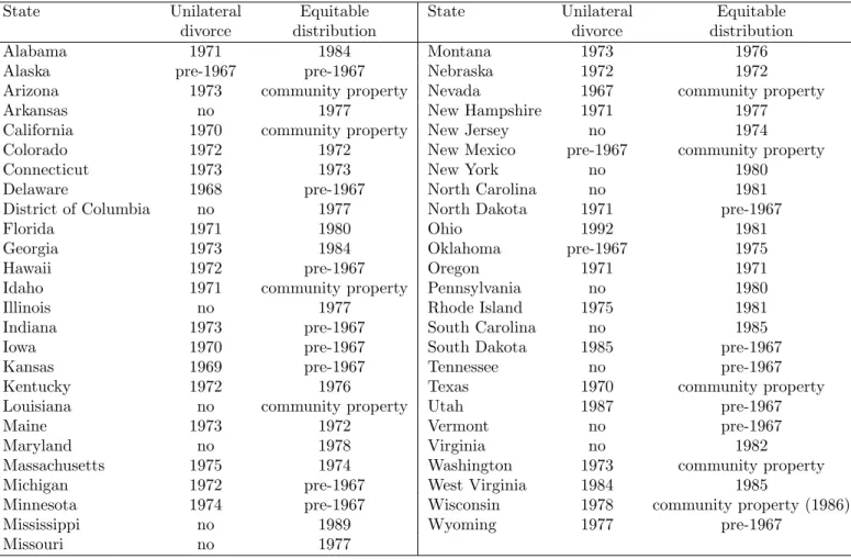
Over the decades of analysis, the legal regimes governing the grounds for divorce in the United States can be described as mutual consent regimes or unilateral divorce regimes. Prior to the 1960s, state regulation allowed divorce only under mutual consent, which permits divorce when both husband and wife agree to it or based on fault grounds, such as adultery or domestic violence. The late 1960s brought about the start of the so-called “unilateral divorce revolution,” which allows one party to obtain divorce without the consent of the other. From 1970 to 1990, the number of states allowing unilateral divorce grew from three to thirty-five (see Table 7 in Appendix F, which illustrated the considerable variation in the content of these laws across states and over time).
occurred in the 1970s was caused by unilateral divorce.2 Making divorce easier may also affect allocations within marriage, which could explain part of the decline in female suicide rate and domestic violence associated with the reforms (Stevenson and Wolfers 2006). However, research on how unilateral divorce affects the labor supply of women is not conclusive (cf. Gray 1998, Stevenson 2008).
Both an increase in the risk of divorce and a change in intra-household allocations due to divorce law reforms may affect household intertemporal behavior. Yet, there is little research on this subject. Stevenson (2007) finds that the introduction of unilateral divorce negatively affects the propensity to undertake marriage-specific investments, such as supporting a spouse through school or buying a home (depending on the property division regime).
1.2
Property Division Laws
Property division regimes over the period of analysis can be broadly classified into three main systems:
a) Title-based regimes, in which assets are allocated according to the title of ownership; b)Community property regimes, in which marital assets and debts are divided equally between the spouses, under the presumption that they are jointly owned;
c) Equitable distribution regimes, in which courts have discretion in dividing marital assets in order to achieve equity. This process may result in equal division or in a division that favors either the spouse who contributed the most to the purchase of the asset or the one in higher financial need.
At the turn of the 20th century, property division based on the formal title to the property was the dominant legal regime, with the exception of eight states, primarily those with a French or Spanish colonial legacy, such as Louisiana, New Mexico or California, which had community
2By the Coase theorem, the change from mutual consent divorce to unilateral divorce should not affect the
probability of divorce since couples should always be able to achieve the efficient outcome (Becker 1991). For the Becker-Coase theorem to hold, a number of strong assumptions are needed (Clark 1999, Chiapporiet al. 2007 and Fellaet al. 2004). In cross-sectional analysis, unilateral divorce states did not have higher divorce rates (Peters 1986 and 1992, although see Allen 1992). Also, the empirical association between unilateral divorce and higher divorce rates in the state-level panel data (Friedberg 1998) may be driven by pre-existing trends in divorce rates (Wolfers 2006), apart from a short-term impact, which suggests that unilateral divorce increased the probability of divorce for couples that were already married (Mechoulan 2006). The difference between short-term and long-term effects may be driven by changes in the likelihood of marriage (Rasul 2003) and in the quality of matching in the marriage market.
property regimes. Over the course of the century, and in particular following the federal Uniform Marriage and Divorce Act (UMDA) of 1970, title-based states shifted towards equitable distribu-tion (Golden 1983, Turner 1998).3 The UMDA, which were intended to favor secondary earners in divorce settlements, created the legal ground for the introduction of equitable distribution in all states: in 1989, Mississippi was the last title-based state to transition into equitable distri-bution (American Bar Association, 1977-2005).4 In Appendix A, I illustrate how the timing of
the transition from title-based regime into equitable distribution is uncorrelated with pre-reform proxies for the economic condition of women in each state.5
From a theoretical perspective, the literature suggests that property division rules to influence both the accumulation of assets (Dnes 1999, Aura 2003) and marital sorting (Chiappori et al.
2008). While the reforms in property division rules have not been subject of empirical analysis, their cross-sectional variation has been used as a distribution factor in intra-household bargaining (Chiappori et al. 2002) and appears to influence the way unilateral divorce affects female labor supply (see Gray 1998, although Stevenson 2008 finds no differential effect of unilateral divorce across property division rules).
2
The Model
To identify the channels through which divorce laws affect household behavior and welfare, I develop a dynamic model of household choice in which spouses jointly decide how much to save, how to allocate consumption and whether or not to work. The model represents the behavior of two individuals, husband H and wifeW, who are married at time 1 and live until time T. In every period from time 1 to T, the household chooses how much to save, how to allocate private consumption between the spouses and whether to stay together or divorce. Between time 1 and
3These legal reforms were salient to U.S. households. For instance, between June and July 1980, when equitable
distribution was introduced in New York state, seven articles were published inThe New York Times regarding this legal change. Between 1974 and 1990 eighty articles fromThe New York Timeshad either “marital property” or “divorce and dissolution” as their focus (http://www.lexisnexis.com).
4These reforms can be seen as a further expansion in the property rights of women after the long process
of rights acquisition that commenced in the middle of the 19th century and granted women control over their property and earnings (Geddes and Lueck 2002, Doepke and Tertilt 2009, Fernandez 2009).
5Prenuptial agreements were likely to have only a minor incidence, because they were not consistently enforced
by courts until the 1980s. Since the 1983 Uniform Premarital Agreements Act, the enforcement of prenuptial agreements has become more likely.
time T −R, the household also makes decisions about the wife’s labor supply. Husbands in this model always work until they retire. From time T −R+ 1 to T, spouses are retired.
2.1
Preferences
Both husband and wife derive utility from own consumptioncj and disutility from own labor force participationPj for j =H, W. Preferences are separable across periods of time and states
of the world.
Each spouse has a subjective taste-for-marriage parameterξtj, which evolves over time. This parameter reflects the spouses’ affection for one another and their attachment to marriage based on other idiosyncratic factors (e.g. fear of the social stigma associated with divorce, concerns about the wellbeing of the children).
Period utility takes the form
ujmarried =u(cjt, Ptj) +ξtj ujdivorced=u(cjt, Ptj).
The taste shocks follow a random walk stochastic process, which captures the persistence in the taste for the current marriage:
ξtj =ξtj−1 +jt, ξ1j =1 where jt is distributed as N(0, σ2) for j =W, H.
The utility function u(c, P) is Constant Relative Risk Aversion (CRRA) and is separable in consumption and participation in the labor market:
u(c, P) = c
1−γ
1−γ −ψP, with γ ≥0 and ψ >0.
2.2
Economies of Scale and Children
Spouses benefit from economies of scale in consumption: for a given level of household expenditurex, spouses’ consumption depends on the household inverse production function
x=F(cH, cW)e(k) = (cH)ρ+ (cW)ρ
1
Withρ≥1, this functional form implies that, for a given level of expenditure, a couple is able to consume more than what it could consume if spouses were living separately. The magnitude of economies of scale in the household depends on the consumption gap between spouses: if one spouse does not consume anything, there are no economies of scale. Economies of scale are maximized when spouses consume the same amount. Children affect household consumption according to an equivalence scale, denoted as e(k) (where k stands for “kids”).
Childbirth occurs at predetermined ages of the parents and fertility is exogenous. Previous literature has indicated that the introduction of unilateral divorce did not seem to have an impact on marital fertility, but it affected the selection into marriage (cf. Alesina and Giuliano 2009). Because the sample only includes couples married before the reforms, this selection mechanism does not influence my analysis.
2.3
Income over the Life Cycle
Each spouse’s labor income (yj forj =H, W) depends on her human capital (hj) and on her
permanent income (zj):
ln(yjt) =ln(hjt) +zjt.
Spouses experience permanent income shocks, which follow a random walk process:
ztj =ztj−1+ζtj and z1j =ζ1j (1)
in which ζtj is i.i.d. as N(0, σ2
ζj) and is correlated between spouses.
Human capital is accumulated through labor force participation. The law of motion for each spouse’s human capitalhj is:
ln(hjt) =ln(htj−1)−δ·(1−Ptj−1) + (λj0+λ1j ·t)·Ptj−1.
If a woman participated in the previous period, her human capital increases at a rateλW
0 +λW1 t.
If she did not, her human capital depreciates at a rate of δ. Since men always work until they retire, PH
pre-retirement income in every subsequent period .
If a woman works, the household faces childcare expenses dk.
2.4
Budget Constraints
In marriage, the budget constraints depend on the property division regime. The general form of the budget constraint is:
At+1−(1 +r)·At+xt=yHt + (y W t −d k t)·P W t . (2)
In a title-based regime, spouses save in separate “accounts” AH and AW that have the same
market rate of return r. Thus, At = AHt +AWt . If divorce were not an option, spouses would
be indifferent between the two accounts. Since divorce is possible, in each period spouses make portfolio choice decisions over what fraction of household assets to allocate the husband and the wife. Upon divorce, each spouse retains her own assets.
In equitable distribution and community property states, assets are treated as jointly owned upon divorce; thus, spouses save jointly.
After divorce, spouses live off their individual income and assets. They both contribute to the consumption of their children as a fraction of their own consumption (which is meant to capture the cost of child custody and of child support) according to the equivalence scale e(k) and they share childcare expenses. The budget constraint becomes:
Ajt+1−(1 +r)·Ajt+cjt ·e(kt) = (ytj− dk t 2 )·P j t. j =H, W (3)
Each spouse’s level of assets in that first year depends on the property division regime. Upon divorce, wealth is divided according to the state’s law, unless spouses reach an agreement on an alternative division:
a) in a title-based system, spouses maintain their own “account”Aj;
b) in community property, assets are divided equally;
c) in equitable distribution, assets are divided but spouses are ex ante uncertain about exact shares. This is meant to capture the fact that “the essential feature of equitable distribution is
the absence of fixed rules for the division of property” (Brake 1982) and that under equitable distribution between half and two thirds of the property is usually assigned to the spouse with the highest earnings (Woodhouse and Fetherling 2006).
At the time of marriage, spouses cannot commit to dividing property differently from what dictated by the law in case of divorce. This assumption reflects the fact that prenuptial agree-ments were rarely enforced before the mid-1980s and remain infrequent today (Mahar 2003). I discuss the welfare implications of prenuptial agreements in a counterfactual simulation exercise in Section 5.
2.5
Problem of the Divorcee
I now characterize the value of being divorced, given state variables ω. In this problem,
ωt={AHt , AWt , ztH, ztW, ξtH, ξtW, hWt ,Ωt} where Ωt represents the vector of divorce laws at time t.
In each period t, a divorcee has an exogenous probability πjtΩ of remarrying another person. The probability of remarriage depends on gender, age and the divorce law regime. If remarriage occurs, it is an absorbing state and the problem is analogous to the one of a married couple with no possibility of divorce and no shocks in the taste for marriage.6 In each period, the divorcee
chooses consumption, savings and whether or not to work (if she is a woman). Thus, the value of being divorced at time t is:
VtjD(ωt) = maxcjD t ,P jD t ,A jD t+1 u(c jD t , P jD t ) +β n πjt+1Ω E[VtjR+1(ωt+1|ωt)] + (1−π jΩ t+1)E[V jD t+1(ωt+1|ωt)] o
s.t. budget constraint in divorce (3), for j =H, W.
The budget constraint depends on the property division regime at the time of divorce.
2.6
Household Planning Problem
The couple’s planning problem depends on the current divorce law regime. In mutual consent divorce, the couple remains married unless both spouses want to divorce; in unilateral divorce,
6The value of being remarried isVjR
t (ωt) =u(cj∗R, Pj∗R) +βE[VtjR+1(ωt+1|ωt)] forj=H, W, from the solution
to the problemVtR(ωt) =maxcHR
t ,cW Rt ,PtW R,ARt+1θu(c
HR
t , PtHR) + (1−θ)u(cW Rt , PtW R) +βE[VtR+1(ωt+1|ωt)])
the couple divorces even ifjust one spouse wants to divorce.
The household solves a constrained Pareto problem, in which the husband’s Pareto weight is indicated byθ and the wife’s weight by 1−θ.7 The parameter θ is determined exogenously.8
Define qt = {cHt , cWt , PtW, AHt+1, AWt+1, Dt} the vector of variables over which the household
maximizes, in which Dt represents the divorce decision at time t.
2.6.1 Mutual Consent Regime
In the mutual consent divorce regime, state variables are
ωt ={AHt , AWt , ztH, ztW, ξtH, ξtW, hWt ,Ωt}, where Dt equals 1 if divorce occurs and 0 otherwise. A
couple that enters periodt as married solves:
Vt(ωt) = maxqt (1−Dt) θ u(cHt , PtH;ξtH) + (1−θ) u(ctW, PtW;ξtW) +βE[Vt+1(ωt+1|ωt)] +Dt θu(cHt , PtH) +βE[VtHDR+1 (ωt+1|ωt)] + (1−θ)u(cWt , PtW) +βE[VtW DR+1 (ωt+1|ωt)]
s.t. budget constraint in marriage (2) oif Dt = 0
budget constraints in divorce (3) for j =H, W u(cH t , PtH) +βE[VtHDR+1 (ωt+1|ωt)]> VtHM(ωt) u(cW t , PtW) +βE[VtW DR+1 (ωt+1|ωt)]> VtW M(ωt) AHt +AWt =At if Dt = 1 where VtjM(ωt) =u(c ∗j t , P ∗j t ;ξ j t) +βE[V j t+1(ωt+1|ωt)]
7 My formulation is a special case of the collective model with non-participation, examined in Blundellet al.
(2007), extended to a dynamic framework and subject to constraints that are imposed by the divorce option.
8For computational tractability, I will assume that each marital cohort has one value ofθ, which is exogenously
determined (e.g. Del Boca and Flinn, 2009). The values of the Pareto weights may be the ones that allow clearing of the marriage market (Chooet al. 2008) or can result from intra-household bargaining at the time of marriage based on non-cooperative threat points (Lundberg and Pollak 1993).
is each spouses’ value of marriage that is obtained by solving the problem for Dt = 0. The
continuation value is Vtj+1(ωt+1) = DtVtjD+1(ωt+1) + (1−Dt)VtjM+1(ωt+1) for j = H, W and ∀t and
∀ωt. Hence, the continuation value for the marriageVt+1is given by the weighted sum of spouses’
continuation values in marriage:
Vt+1(ωt+1) =θ VtH+1(ωt+1) + (1−θ)VtW+1(ωt+1)
∀t= 1, ...T −1 , which depend on marital status
Vtj+1(ωt+1) = Dt+1VtjD+1(ωt+1) + (1−Dt+1)VtjM+1(ωt+1)
forj =H, W.
The allocation in marriage in mutual consent divorce corresponds to the Pareto-optimal allocation. In every periodt, the couple remains married unless both spouses prefer the divorce allocation, described in Subsection 2.5.
If spouses disagree about the divorce under the default property division rule (i.e. one spouse has a binding divorce constraint), the spouse who wants to divorce can persuade the other by offering her (him) a larger fraction of the household assets compared to the one dictated by the law, to make her indifferent between remaining married and divorce.
2.6.2 Unilateral Divorce Regime
In a unilateral divorce state, the couple maximizes the weighted sum of spouses’ utilities in marriage under the constraint that both spouses must prefer the marriage allocation to the value of being divorced. Because the marriage allocation has to satisfy these participa-tion constraints, the soluparticipa-tion may depart from the Pareto optimal allocaparticipa-tion. The formulaparticipa-tion of the unilateral divorce case follows from the literature on risk sharing with limited commit-ment (e.g. Ligon et al. 2000), which has been applied to models of intra-household allocation (Ligon 2002, Mazzocco 2007, Mazzocco et al. 2009, Gallipoli and Turner 2011). Define Mtj (for
j = H, W) two additional state variables in this problem. Mtj > 0 indicates that the intra-household allocation departs from the solution to the intertemporal Pareto problem because of
the presence of binding participation constraints between time 1 and timet. State variables are
ωt={AHt , AWt , ytH, ytW, ξtH, ξtW, hWt ,Ωt, MtH, MtW}.
The couple solves:
Vt(ωt) = maxqt (1−Dt) (θ+MtH)u(cHt , PtH;ξtH)+ (1−θ+MtW) u(cWt , PtW;ξtW) +βE[Vt+1(ωt+1|ωt)] +Dt (θ+MtH)u(cHt , PtH) +βE[VtHDR+1 (ωt+1|ωt)] +(1−θ+MtW)u(cWt , PtW) +βE[VtW DR+1 (ωt+1|ωt)]
s.t. budget constraint in marriage (2)
u(cHt , PtH;ξtH) +βE[VtH+1(ωt+1|ωt)]≥VtHD(ωt) u(cW t , PtW;ξtW) +βE[VtW+1(ωt+1|ωt)]≥VtW D(ωt) if Dt= 0
budget constraints in divorce (3) for j =H, W
AHt +AWt =At if Dt= 1 where VtjM(ωt) =u(c ∗j t , P ∗j t ;ξ j t) +βE[V j t+1(ωt+1|ωt)]
is each spouses’ value of marriage that comes from solving the problem for Dt = 0. The
contin-uation value isVt+1(ωt+1) =θ VtH+1(ωt+1) + (1−θ)VtW+1(ωt+1) ∀t= 1, ...T −1 , where
Vtj+1(ωt+1) =Dt+1VtjD+1(ωt+1) + (1−Dt+1)Vt+1jM(ωt+1) for j =H, W.
In every period t, the couple remains married only if both spouses prefer the marriage allo-cation. If, given the solution to the unconstrained problem, spouses disagree about divorcing, then the spouse who wants to remain married can persuade the other by offering her (him) a larger fraction of the couple’s resources than the one established by the Pareto-efficient household planning problem. Hence, the ratio of spouses’ marginal utilities of consumption shifts, as de-scribed in the literature on risk sharing with lack of commitment (Kocherlakota 1996). [INSERT DESCRIPTION OF EQUILIBRIUM]
Assume that, given the solution to the unconstrained problem, the wife wants to remain married while the husband wants to divorce (i.e. he has a binding participation constraint). Then, she offers the husband an allocation that makes him indifferent between marriage and divorce. This corresponds to the solution to a Pareto problem in which spouses’ weights correspond to (θ+MtH+µHt ) and (1−θ+MtW+µWt ), whereMtj =Ptτ−=11 µjτ, forM1j = 0 andµjt >0 is spouse’sj
binding participation constraint at timet, forj =H, W (Marcet and Marimon 1992). If such an allocation is infeasible, i.e. if any allocation that satisfies both spouses’ participation constraints violates the household’s intertemporal budget constraint, then divorce occurs. Appendix B provides a detailed description of the solution algorithm adopted.
2.7
Divorce Laws and Household Outcomes
The model has implications for three observable elements of household behavior: divorce, assets accumulation and female labor supply. These implications derive from both the direct effect of each law and the interaction effects between grounds for divorce and property division laws.
Because utility is not perfectly transferable, in this model unilateral divorce increases the likelihood of divorce. In addition, it changes the terms of intra-household allocation. Under mutual consent divorce, the intra-household allocation is fully determined by the Pareto weights. Once unilateral divorce is introduced, the ratio of the marginal utilities of consumption shifts as spouses’ participation constraints become binding, to allow the marriage to continue.9 For
a given θ, property division laws then only affect the intra-household allocation if there is a unilateral divorce, as the consumption share shifts in favor of the spouse who would get more resources in divorce than in the initial intra-household allocation. Equal division of property increases the likelihood that the participation constraints becomes binding for the spouse with a smaller share in household resources, as it improves the outside option VjD.
Divorce laws affect assets accumulation in two ways. First, they regulate the fraction of household total assets each spouse can access upon divorce. Second, they influence the amount
9Under mutual consent divorce, uc(cH,PH)
uc(cW,PW) =
1−θ
θ , because spouses cannot exercise the threat of divorcing
without the consent of the other party and thus divorce cannot be a relevant threat-point of intra-household negotiation. Once unilateral divorce is introduced, the ratio becomes uuc(cH,PH)
c(cW,PW) = 1−θ+MW t θ+MH t .
of total savings that a household accumulates. In a title-based property division regime, the household can decide what share of the couple’s assets to allocate to each spouse. To allow spouses to smooth consumption upon divorce, their own assets are increasing in their Pareto weight and thus in their share of consumption in marriage. In equitable distribution and community property states, households can only choose thetotal amount of savings and courts decide spouses’ shares. Thus, only a spouse with a relatively low Pareto weight will benefit from equal division of property compared to a title-based regime (see Figure 2). While in mutual consent the impact of property division laws is attenuated by the fact that spouses may renegotiate the divorce settlements if one spouse does not want to consent to divorcing, in unilateral divorce property division laws directly affect all divorce settlements, and are more likely to influence household behavior.
By altering spouses’ individual resources, divorce laws also influence the incentives to save during marriage. Relative to a title-based regime, equal division of property imposed by courts alters the returns on savings. In marriage, each spouse’s share in household consumption is increasing in his/her Pareto weight. Thus, an equal division of assets acts as a tax on savings for the spouse who consumes more in the marriage (the one with the higher Pareto weight) and as a subsidy for the other. Similarly to a change in the market return on assets or to a tax on savings (Bernheimet al. 2002), such a decrease has a substitution effect (consumption is cheaper at time
tthan at time t+ 1, which may decrease savings) and an income effect (for a net saver, resources available at timet+ 1 are lower, which may increase savings). More risk-averse households would respond to equal division of property in unilateral divorce by accumulating more savings, while less risk-averse one would respond by accumulating less assets (this is the interaction effect). Moreover, if divorce imposes upfront costs (independently of the property regime), an increase in the likelihood of divorce may lead households to save more (Cubeddu and Rios-Rull 1997 and 2003, Gonzalez and Ozcan 2008) independently of the way property is divided (this is the main
effect of unilateral divorce).
Turning to female labor supply, if women have fewer resources upon divorce than in marriage (e.g. if they benefit from a share of the husbands’ income during marriage), they have an incentive to work to accumulate human capital when facing an increase in the risk of divorce (as verified in Johnson and Skinner 1986). However, the more favorable to women the property regime is, the weaker this channel would be, since tangible assets already provide women with insurance
in case of divorce.10 In addition, a woman’s likelihood of employment isdecreasing in her share of household resources, which is related to the weight of the wife’s disutility of working in the household planning problem. By increasing a woman’s value of divorce, divorce laws that favor women may lead to an increase in their share in household resources and a reduction in her likelihood of employment.
3
Data and Empirical Analysis of the Reforms
In this section, I illustrate how panel variation in U.S. divorce laws is correlated with a number of changes in the economic behavior of households. According to the dynamic model described above, the effect of divorce laws reforms on wealth accumulation and on female labor supply is closely tied to the structural parameters of the model. In this section, I will examine these two outcome variables. Appendix D illustrates more evidence on hours worked by husbands and hours devoted to housework by both husbands and wives, which are not included in the model but appear to also change in response to changes in divorce laws, in a way that is consistent with a change in intra-household allocations.
3.1
The Data
I use data from the Panel Study of Income Dynamics (PSID), the National Longitudinal Survey of Mature Women (NLS-MW), and the National Longitudinal Survey of Young Women (NLS-YW). These surveys provide longitudinal information on U.S. households from the end of the 1960s until the 2000s. In this paper, I use 26 waves of the PSID (between 1968 and 1993), 19 waves of NLS of Mature Women (between 1967 and 1999), and 20 waves of NLS of Young Women (between 1968 and 1999).
The PSID provides key information on labor force participation (in addition to hours of work
10This model does not consider alimony. Alimony in this context would imply a reduction in the scope for
self-insurance for women and an increase in women’s bargaining power in marriage when unilateral divorce is allowed. Data on alimony payments show that these were generally infrequent transfers. For instance, in the National Longitudinal Survey of Young and Mature Women only 10% of divorced women ever report receiving alimony between 1977 and 1999, for a median payment is 4,000 real 2008 dollars, approximately 15% of the divorcee’s household income. Child support is usually a larger transfer from the non-custodial parent to the parent who is granted custody of the children. Del Boca and Flinn (1995) examine a sample of divorce cases in Wisconsin between 1980 and 1982, where the average child support transfer is about 20% of the father’s income.
and hours of housework examined in Appendix D). I use data until the 1993 wave, after which several questions were significantly modified in the survey. The NLSW provides uniquely rich data on household wealth. The NLS-MW and NLS-YW are part of the Original Cohorts of the National Longitudinal Surveys. The NLS-MW was administered from 1967 to 2003 on an initial sample of 5,083 women who were between 30 and 44 years of age in 1967. The NLS-YW was administered from 1967 to 2003 to an initial sample of 5,159 women who were between 14 and 24 years of age in 1968. These surveys provide rich data on household asset holdings, which is not available in other longitudinal surveys from the 1970s and 1980s. Since the NLS does not disclose state identifiers, I matched women to their state of residence using the geographical variables provided in the surveys.11
Since the model takes household formation as exogenous, the empirical analysis only considers couples that marriedbefore the legal reforms took place: divorce laws may in fact also affect the decision to marry and the sorting in the marriage market. Thus, my sample includes couples in their first marriage married before the introduction of unilateral divorce in their state, before changes to divorce settlement laws were made.
The PSID provides detailed longitudinal information on female employment and divorce. Table 1 summarizes characteristics of the pooled sample of the 3,858 women I analyze. Average female employment in the sample is 54%.
In the NLSW, the women I analyze are slightly older than those in the PSID sample due to the sampling age of the initial cohort. Data on wealth is collected for a subset of years, leaving us with assets information for 4,538 couples.12 Assets include real estate, financial assets and business assets. Table 1 reports the average and median characteristics of this sample. Household assets average almost 70,000 and income averages approximately 38,000, both in real 1990 dollars. Asset holdings peak when women are 64 at a mean level of 127,000 real 1990 dollars. Seventeen
11The variables that I use to match women to their state of residence are the size of the labor market in the
1960 Decennial Census in the area of residence, an index of the demand for female labor in the area of residence and the Census division of residence. A similar approach is used in Powers (1998) on the NLS-YM. I thank Jeff Gray for providing the list of geographical characteristics at the Primary Sampling Unit (PSU) level and the PSU-state matches. Since this information is only available for the waves between 1967 and 1971, I can only identify the state of residence for those survey respondents who did not move to another state after 1971. Thus, I match 10,086 women out of 10,242 at least once in the sample, but for a total of 2,856 women, the state of residence eventually becomes unavailable once they report having moved.
12In the NLS-MW assets are recorded in 1967, 1971, 1972, 1977, 1982, 1987, 1989, 1995, 1997, 1999. For
percent of households in the pooled sample hold zero or negative total assets at a point in time.
3.2
Empirical Analysis
I exploit the variation in divorce laws across states and over time, as summarized in Appendix Table 7. Unilateral divorce was introduced at different points in time in thirty-three states between 1967 and 1992. In the same period, all twenty-seven states that had a title-based property division system adopted equitable distribution. The sources of variation that I use are the introduction of unilateral divorce in different pre-existing property regimes (primarily community property and title-based regimes) and the adoption of equitable distribution under different legal grounds for divorce (mutual consent and unilateral divorce).
Variation in divorce laws is concentrated among the following cases:
a) households which experience the introduction of unilateral divorce while in a title-based regime (398 households in the NLSW, 290 households in the PSID) or while in a community property regime (653 households in the NLSW, 573 households in the PSID);
b) households which experience the introduction of equitable distribution in mutual con-sent states (1,149 households in the NLSW, 1,701 households in the PSID) or in unilateral divorce states (206 households in the NLSW, 249 households in the PSID);
c) households that experience the introduction of both equitable distribution and unilateral divorce in the same year (233 households in the NLSW, 178 households in the PSID).13
Other combinations of legal changes affected only a small number of households. A few households experienced the transition into unilateral divorce as equitable distributions states (12 households in the NLSW and 87 households in the PSID). Finally, only a few households entered a community property regime during the sample period, since Wisconsin was the only state that changed from an equitable distribution to a community property regime in 1986. Such observations are insufficient to provide accurate data for such a quasi-experiment; thus, they will not be used for causal interpretation.
3.2.1 Household Wealth
To examine the impact of divorce laws on couples’ accumulation of assets, I estimate the following equation for household iin state s and in year t:
assetsi,s,t=β1U nilaterals,t+β2(U nilateral·Com.P rops,t) (4)
+β3(U nilateral·Eq.Distrs,t) +β4Eq.Distr.s,t+β5Com.P rop.s,t
+γ0Zi,t+δt+fi+cs+i,s,t.
The dependent variable assets represents the total net assets of a married couple, reported in real 1990 dollars. Assets are measured in levels, to include households with net debt (negative assets).14 The vectorZ contains a set of controls for spouses’ age, years since marriage and family
structure; δt denote year fixed effects; cs state fixed effects and fi household fixed effects.15
I consider a vector of property division and grounds for divorce regimes; the excluded category is a title-based mutual consent system:
a) Coefficient β1 (U nilateral) captures the effect of unilateral divorce with respect to
mutual consent divorce in title-based states.
b) Coefficient β2 (U nilateral·Com.P rop) captures the additional (interaction) effect of
unilateral divorce in community property. The total effect of introducing unilateral divorce in such states is given byβ1+β2. The coefficientβ2 captures the impact of the change in individual
returns on assets that occurs when unilateral divorce is introduced in this property division regimes.
c) Coefficientβ3 (U nilateral·Eq.Distr) captures a similar effect asβ2, plus the impact of
uncertainty in the allocation of assets upon divorce, since in equitable distribution states judges have more discretion in the allocation of property and tend to favor the primary earner.
d) Coefficient β4 (Com.P rop.) measures the average difference in assets between
title-based and community property states in mutual consent regimes. Since its estimation is not
14Because this analysis is conducted on a sample of married samples, I consider the possibility that the results
may be driven by non-random attrition due to diverse characteristics of divorcing couples across legal regimes. I use Inverse Probability Weighting to ensure that this is not the case (Appendix C).
15Because I restrict the sample to couples married before the reforms, it is important to control for life-cycle
effects and for the duration of the marriage, to avoid mechanically attributing the impact of this feature of the sample to changes in divorce laws .
based on quasi-experimental variation, it has no plausible causal interpretation.16
e) Coefficient β5 (Eq.Distr.) measures the average difference in wealth due to the
intro-duction of equitable distribution in mutual consent regimes. The total impact of the introintro-duction of equitable distribution in unilateral divorce states is also captured byβ3+β4.
Table 6 reports the results of the estimation of Equation (4) using fixed-effect OLS regressions for different specifications. Column 1 is the baseline specification, which includes age dummies for the wife, year fixed-effects and individual fixed effects as controls. Column 2 controls for a polynomial in the husband’s age, which is missing for some couples of the sample. Column 3 adds state fixed effects. Column 4 also includes a 4th degree polynomial in the years of marriage. Appendix C presents a set of robustness checks on these results.
The coefficient β1, which represents the effect of unilateral divorce in title property states,
is equal to -5,959 (Column 1) and is not statistically significant. In contrast, coefficients β2
and β3 are equal to 18,118 and 14,573 real dollars and are statistically significant at the 5%
level, suggesting that the interaction effect of unilateral divorce in equitable distribution and community property states is the most relevant. The average increase in household assets in community property states and equitable distribution states when unilateral divorce is introduced (β1+β2 and β1 +β3) is equal to 12,159 real dollars and 8,614 real dollars respectively.17 The
effect of the transition from title-based regimes to equitable distribution (β5) is equal to -13,898
real dollars but is generally not statistically significant. Figure 6, panel a, illustrates an the dynamic impact of unilateral divorce in community property states obtained from estimating, on the sample of households for which Com.P r.= 1:
assetsi,s,t =βpreU ni. within3yrss,t+
15+
X
τ=0(3)
βτU ni. f or τ to(τ+ 2)yrss,t+γ0Zi,t+δt+fi+cs+i,s,t,
whereU ni. within3yrsis equal to 1 when householdi in yeart will experience the introduction of unilateral divorce within the subsequent 3 years and 0 otherwise, whileU ni. f or τ to(τ+ 2)yrs
16The coefficient would be identified by households that change state of residence. As explained above, changes
in the state of residence are not measured after 1971. Furthermore, only Wisconsin introduced community property in this sample period (1986), following the introduction of unilateral divorce.
17Similar findings are confirmed from estimating Equation (4) using median regressions (without individual fixed
effects), as shown in the Appendix. However, the coefficients estimated using median regression are substantially smaller than those obtained from the OLS, suggesting that wealthy households exhibit a greater response to the reforms.
equals 1 if unilateral divorce has been introduced in the past τ to τ + 2 years and 0 otherwise. The figure shows no increase in assets for the first 6 years since the reform nor forβpre, and then
a smooth raise in the accumulation of assets over time.
The finding that households who live in community property states and equitable distribution states seem to modify their asset accumulation behavior in the presence of unilateral divorce, while no effect is observed in title-based states, is consistent with the hypothesis that the dis-tribution of resources in divorce at baseline does not match the one in marriage in such states, leading to a change in the returns on savings once unilateral divorce is introduced in community property states. However, changes in total savings alone do not tell us which spouse obtains more resources in marriage.
3.2.2 Employment of Married Women
The likelihood of employment of married women may be affected by divorce laws, depending on the distribution of Pareto weights. To examine the impact of the legal regime on the female labor supply, I estimate the following equation using a linear fixed effects probability model:
P(employmenti,s,t= 1) =β1U nilateral+β2(U nilateral·Com.P rop.s,t) (5)
+β3(U nilateral·Eq.Distr.s,t) +β4Com.P rop.s,t+β5Eq.Distr.s,t
+γ0Zi,t+δt+fi+cs,
where employmentis equal to 1 if the woman is employed and to 0 otherwise. This equation is analogous to Equation (4). Coefficient β1 is meant to capture the effect of the introduction of
unilateral divorce that is common in all states. Coefficientsβ2 and β3 identify theinteraction
ef-fect that unilateral divorce may have in states with community property or equitable distribution respectively. Thus, the total effect of introducing unilateral divorce in a community property state is given byβ1+β2, in equitable distribution β1+β3. Coefficientβ4 is not identified by any
source of exogenous variation. Finally, coefficientβ5 captures the impact of introducing equitable
distribution while in a mutual consent regime.
The result of estimating equation (5) suggests that generally unilateral divorce has no statisti-cally significant impact on female employment. However, in community property states women’s
employment declines by 5.8 percentage points when unilateral divorce is introduced; the effect is statistically significant at the 1% level (Table 6). This finding is robust to controlling for the number of children in the household (Columns 6, 7 and 8), for state fixed effects (Column 7 and 8) and for the time elapsed since marriage (Column 8). Appendix C illustrates a set of robustness checks.
Figure 6, panel a, illustrates an the dynamic impact of unilateral divorce in community property states obtained from estimating, on the sample of households that satisfyCom.P r.= 1:
P(employmenti,s,t = 1) =βpreU ni. within3yrss,t
+
15+
X
τ=0(3)
βτU ni. f or τ to(τ+ 2)yrss,t+γ0Zi,t+δt+fi+cs,
where U ni. within3yrss,t which is equal to 1 when household i in year t will experience the
introduction of unilateral divorce within the subsequent 3 years. The figure shows no significant coefficient for βpre, and then an immediate drop in employment which dies off over time.
This findings suggests that unilateral divorce may have increased women’s allocations in marriage in those states where women received 50% of household assets upon divorce. As a result, women become less likely to work. This fact supports the hypothesis that women’s Pareto weight is low enough compared to their husband’s weight, so that unilateral divorce with equal division of property improves their condition with respect to the intra-household allocation. First, women benefit from the post-reform intra-household allocation thanks to the more favorable divorce outside option compared to the initial marriage allocation. Second, the additional assets awarded by courts reduce women’s need for accumulation of human capital as self-insurance against the risk of loss of consumption in the event of a divorce. Both channels contribute to reducing women’s employment.
This result is consistent with what described by Chiappori et al. (2002), who examine the labor supply of a cross-sectional sample of couples in the PSID and find that female labor supply is lower in community property states than in other states. Hence, Chiappori et al. (2002) focus on cross-sectional variation in property division rules as a distribution factor in a static model, without examining the impact of introducing unilateral divorce. The variation exploited
in this study allows to also identify interaction effects of property division laws and ground for divorce laws, since I observe both the introduction of unilateral divorce in community property or title-based states and the introduction of equitable distribution in mutual consent and unilateral divorce states. The theory suggest that such interaction effects are crucial to interpret the impact of changes in divorce laws for couples married before the reforms: as the model implies, the presence of unilateral divorce allows the divorce allocation to affect the one in marriage, while couples who live in a mutual-consent regime are unlikely to be affected by a change in property division rules.
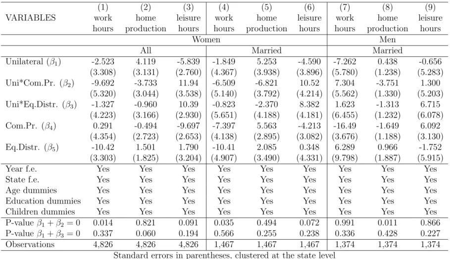
Interpreting the decline in female employment as a shift in intra-household allocation in favor of women, while common in the literature (Chapporiet al. 2002, Lafortuneet al. 2012), requires assuming that women do not entirely substitute market work with housework, in particular if the utility cost of housework is as high as, or higher than, the cost of labor. In Appendix D, I use data on time use from multiple survey based on Aguiar and Hurst (2007) to document that the decline in female employment that we observe when unilateral divorce is introduced in states with an equal division of property regime is associated with a net increase in their leisure time, which was sizable and statistically significant, while only a small and statistically insignificant increase in home production is observed. The increase in the amount of leisure time enjoyed by women reinforces the hypothesis that the decline in female employment may be due to an increase in women’s weight in intra-households decision making, and hence in an increase in their wellbeing.
4
Structural Estimation
Divorce law reforms have two main effects on the outcomes analyzed in the Section 3. The presence of both community property (or equitable distribution, to a lesser extent) and of uni-lateral divorce is associated with more assets and lower female employment than when mutual consent divorce is in force. These changes are not observed when unilateral divorce is introduced in title-based states.
I exploit these facts to estimate the key structural parameters of the model, using indirect inference:
a) the Pareto weight of the husband θ,
b) the standard deviation of the shocks to the taste for marriage σ, c) the utility cost of working ψ.
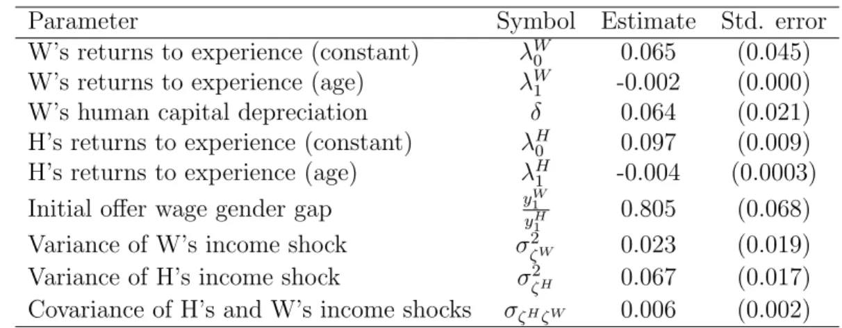
In a first stage, I estimate the parameters of the income process using moments of spouses’ joint income distribution from the PSID (a two-step procedure makes the estimation computa-tionally tractable, see Gourinchas and Parker 2002 and in De Nardi, French and Jones 2010). I account for the selection of women into the workforce using the divorce laws variables that affect women’s decision to work and are excluded from the offer wage equation conditional on their human capital, as illustrated in the model. The parameters estimated in this first step are the variance and covariance of spouse’s permanent income shocks (σ2
ζj for j = H, W and σζHζW),
the returns to labor market experience for each spouse (λj0 and λj1), the depreciation rate of the human capital of women (δ) and the offer wage gender gap at the beginning of the spouses’ career (yW1
yH
1
).
I also select a set of pre-set parameters, as described in Table 3, to simulate the model and estimate the remaining structural parametersσ, ψ, θ.
4.1
Spouses’ Income Processes
The spouses’ income processes parameters allow the model to account for spouses’ incentives to share income risk and for spouses’ wage difference over the life cycle. I estimate the parameters using non-linear least squares (Table 2). Identification of such parameters is described in detail in Appendix E. The estimated offer wage gender ratio at age 23 is 81%. The wage gap first grows and then shrinks over the life cycle, due to a higher λj0 and a lower λj1 for men.18 Third, based
on the estimated variances, the income of men is more variable than that of women. Finally, the estimates reveal a positive covariance in the shocks to the permanent wage of the husband and the wife (the implied correlation is equal to 15%).
18My estimates for the returns to labor market experience for women λW
0 is larger than others reported in
the literature (Eckstein and Wolpin 1989, Attanasioet al. 2008); however, the profile of women’s wages is more concave (λW
1 is smaller than in the literature). Such estimates imply that the average yearly returns to experience
over 30 years of career is 3.4%, compared to 2.7% calibrated in Attanasioet al. (2008). Olivetti estimates the returns to a year of full-time work in a 3% to 5% range. The estimates in this study lie between those by Attanasio et al. (2009) and by Olivetti (2006). The estimate for the depreciation rateδ is roughly comparable to the 7.4% calibrated in Attanasioet al. (2008).
4.2
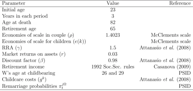
Pre-set Parameters
A group of parameters of the model are set to values drawn from the literature. Table 3 presents the pre-set parameters. To reduce the dimensionality of the problem, I set each period to correspond to 3 years of life. Spouses have the same life cycle: they are 23 years old at time 1; they retire at age 62 (end of period 13) and die with certainty at age 79 (end of period 18).
I calibrate the economies of scale parameter ρ to match the McClements scale, according to which a person living alone spends 61% of what a childless couple spends to achieve the same level of consumption. Such a scale is an intermediate value for the magnitude of economies of scale in the family estimated in the literature (see Fernandez-Villaverde and Krueger 2007). This calibration leads to a parameter value of ρ = 1.4023.19 The McClements scale is also used to
calculate the consumption of the children as a fraction of their parents’ consumption.20
The relative risk aversion parameter γ is set to 1.5 (e.g. Attanasio et al., 2008). I set the annual market rate of return on assets r to 3% and the annual discount factor β to 0.98.
4.3
Indirect Inference
I use indirect inference (Gourieroux et al. 1993) to estimate the key parameters of the model, exploiting the variation provided by the divorce law reforms as the primary source of identification.
First, I solve the dynamic model under mutual consent divorce for vectors of possible values of structural parameters Π = (σ ψ θ)0, given the realizations of the income and taste shocks. Couples are assumed to have no assets at the time of marriage (age 23). I simulate income and taste shocks and use the policy functions to obtain the corresponding profiles of pre-reform household assets, female labor participation and marital status before retirement.21
Second, I solve for the introduction of unilateral divorce at various stages of the life cycle.
19Based on to the McClements scale, 0.61x=cj. Under the assumption that spouses have identical consumption
levels, the household inverse production function becomesx= 21ρcj. Thusρ= log(2)
log( 1
0.61)
= 1.4023.
20A couple with a child aged 0-1 consumes 109% of what a childless couple consumes. The additional fraction
is 18% for each child between 2 and 4 years, 21% between 5 and 7 years, 23% between and 8 and 10, 25% between 11 and 12, 27% between 13 and 15 and 38% between 16 and 18 years.
21I focus on the pre-retirement period for two reasons. First, my estimates in Section 3 are based on a sample
of couples under the age of 65. Second, since attrition for death in my sample is higher after age 65 and it is not taken into account by the model, excluding retired people minimizes the potential impact of attrition.
I again simulate the post-reform behavior of household assets, female labor participation and divorce, at ages that match those observed in PSID data. The underlying assumption is that couples do not change their state of residence in response to or in anticipation of divorce law reforms. This hypothesis appears especially plausible if one considers that most states in the U.S. have relatively long residency requirements before spouses can divorce in the state where they live.
I estimate the same auxiliary model on the simulated data and obtain a vector of auxiliary parameters φsim(Π). The optimal choice of ˆΠ minimizes the distance between the auxiliary
parameters estimated on the actual data and the auxiliary parameters estimated on the simulated data. I choose ˆΠ = ( ˆσ2
ψˆ θˆ)
0 such that:
ˆ
Π =ArgminΠ( ˆφdata−φsim(Π))G−1( ˆφdata−φsim(Π))0 (6)
whereGis a weighting matrix set to be equal to the estimated variance-covariance matrix of the parameters of the auxiliary model.
The auxiliary model includes the two difference-in-differences estimators for the introduction of unilateral divorce in different states at different points in time. To ease the computation and focus on the states that show the sharpest responses, I estimate the parameters on the sample of couples living in community property states.
The auxiliary parameters are {φ1, φ2, φ3, φ4} from the following model:
a) the relative change in household assets when unilateral divorce is introduced
assetsi,s,t=β U nilaterals,t+γ0Zi,t+δt+fi+υ1,i,s,t
φ1 =
β
average assets (7)
where ˆφ1,data = 16%;
b) the response of female participation when unilateral divorce is introduced
employmenti,s,t =φ2U nilaterals,t+γ0Zi,t+δt+fi+υ2,i,s,t (8)
c) the average female participation rate in mutual consent regimes of the pooled sample of women between 23 and 50 years old (to avoid the confounding effect of retirement)
employmenti,s,t =φ3+υ3,i,s,t (9)
where ˆφ3,data = 57%;
d) the average divorce rate in mutual consent regimes of the pooled sample of couples in which women are between 23 and 64 years old
ever divorcedi,s=φ4+υ4,i,s (10)
where ˆφ4,data = 19%.
Equations (7) and (8) are analogous to the reduced-form Equations (4) and (5) from Section 3, estimated on the subsample of households living in community property states.22
4.4
Identification
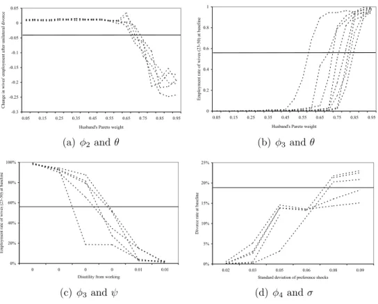
The choice of the auxiliary parameters allows a rather transparent identification of the struc-tural parameters of the model. All parameters of the auxiliary model contribute to the estimation of the structural parameters. However, in some cases, the theoretical link between a structural parameter and an auxiliary parameter is strong and crucial for identification.
The response of wives’ likelihood of employment to changes in such laws provides the infor-mation to identify the parameter θ. Such moment is decreasing in the Pareto weight of men for values of θ that are sufficiently large, namely larger than the husbands’ relative share in household permanent income (and therefore at least larger than 12). If the wife’s Pareto weight is not substantially smaller than the Pareto weight of the husband compared to the relative per-manent incomes, the introduction of unilateral divorce in community property has little effect on her labor supply; such an effect would be positive, in that case, because women may want to accumulate human capital in case divorce occurs. On the contrary, for values of θ sufficiently
22For example, the asset equationassets
i,t=β1U nilaterals,t+β2(U nilateral·Com.P rops,t)
+β3(U nilateral·Eq.Distrs,t) +β4Eq.Distrs,t+β5Com.P rop.s,t+γ0Zi,t+δt+fi+i,t whenCom.P rops = 1
larger than 12 (i.e. when the husband has more decision power) the participation of women drops following the introduction of unilateral divorce. The introduction of unilateral divorce leads to a transfer of resources (consumption of goods and leisure) from the husband to the wife, because the divorce outside options are more favorable to women with respect to their share of resources in marriage at baseline. It follows that the estimated value ofθ will need to be sufficiently larger than 12 to match an auxiliary parameterφ2 =−4.6 percentage points (Figure 1, Panels a and b).
The primary role of the utility cost of participation (ψ) in the model is determining a woman’s labor market participation decision. Since,ceteris paribus, a woman is more likely to participate in the labor market the lower her utility cost of working, the average female employment rate provides information for the structural parameter ψ (Figure 1 panel c). Similarly, the standard deviation of the preference shock parameter (σ) influences the likelihood of divorce. For low values of σ, divorce is an unlikely phenomenon, since few spouses receive negative shocks ξj
sufficiently high to counteract the benefits of marriage that derive from the economies of scale. As
σ increases, the likelihood that a spouse would prefer divorce increases. Therefore, identification of the parameterσ stems from the average divorce rate in mutual consent states (Figure 1 Panel d).
4.5
Results
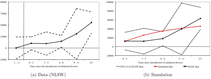
Table 4 illustrates the solution to Problem (6). When unilateral divorce is introduced in the sample, women’s weight in household decision is a third of their husband’s weight. The estimated disutility of working is equal to 0.0033 and the estimated standard deviation of preference shocks is equal to 0.06. This corresponds to a baseline participation rate of 55%, which decreases by 7.2 percentage points after the introduction of unilateral divorce (Table 4). The increase is assets after the reform is equal to 17% in the simulations. Finally, the baseline divorce probability in the estimated model is equal to 21%.
Like in the data, in simulations from the model the accumulation of assets responds slowly to unilateral divorce, while the probability of female employment exhibits a sharp drop (Figures 6 and 6). In the data, the effect of the reforms on employment disappears after 15 years since the reform, while in the model more periods are needed (after 27 years since the reform). This pattern may be explained by the fact that a large stock of women had binding participation constraints