Robust image classification:analysis and applications

(1)

POUR L'OBTENTION DU GRADE DE DOCTEUR ÈS SCIENCES

acceptée sur proposition du jury: Prof. P. Vandergheynst, président du jury

Prof. P. Frossard, directeur de thèse Prof. J. Bruna, rapporteur Prof. N. Paragios, rapporteur

Dr F. Fleuret, rapporteur

Robust image classification: analysis and applications

THÈSE N

O

_{7258 (2016)}

ÉCOLE POLYTECHNIQUE FÉDÉRALE DE LAUSANNE

PRÉSENTÉE LE 16 DÉCEMBRE 2016

À LA FACULTÉ DES SCIENCES ET TECHNIQUES DE L'INGÉNIEUR LABORATOIRE DE TRAITEMENT DES SIGNAUX 4 PROGRAMME DOCTORAL EN GÉNIE ÉLECTRIQUE

Suisse 2016

PAR

(2)

(3)

Acknowledgements

I would like to thank my PhD advisor, Prof. Pascal Frossard, for giving me the opportunity to do a PhD in his research group. I am grateful for his guidance and for giving me the freedom I needed to pursue my research interests. Besides, I was very fortunate to benefit from his experience and insights. I also greatly thank him for providing thorough and detailed feedbacks. I finally thank him for his constant support and consideration, and for always believing in me!

I would also like to thank the members of my thesis committee, Prof. Joan Bruna, Dr. François Fleuret, Prof. Nikos Paragios, and Prof. Pierre Vandergheynst for the time they have taken to review my manuscript, and for their helpful comments.

I would like to thank my colleagues and collaborators from IBM Ireland and Watson; Mathieu Sinn, Bei Chen, Jean-Baptiste Fiot, Horst Samulowitz, Deepak Turaga, as well as all others that I enjoyed talking to during the internships. Many works would not have been possible without their precious help and support. Thanks to Olivier Verscheure for giving me the opportunity to do these internships. I have really enjoyed the many discussions we’ve had, and his constant motivation has always been a great support. Special thanks to Prof. Mike Davies and Prof. Laurent Jacques for the enriching discussions, and for inviting me to Edinburgh and Louvain-La-Neuve.

I also sincerely thank all the current and former members of the lab Ana, Andreas, Beril, Chenglin, David, Eirini, Elif, Ersi, Francesca, Hermina, Jacob, Laura, Luigi, Nikos, Renata, Pinar, Sofia, Tamara, Thomas, Vijay, Xiaowen. I thank Dorina for sharing the office with me during all those years, Stefano and Mattia for the very exciting and entertaining discussions, and Seyed for being a great colleague and a genuinely nice person I enjoyed collaborating with.

Finally, I would like to thank many friends, especially from GMU, who made life in Lausanne very enjoyable. I also greatly thank my brothers, Omar and Hamza, for their constant help and their continuous support. And it is a pleasure to thank my parents and my wife for everything.

(4)

(5)

Abstract

In the past decade, image classification systems have witnessed major advances that led to record performances on challenging datasets. However, little is known about the behavior of these classifiers when the data is subject to perturbations, such as random noise, structured geometric transformations, and other common nuisances (e.g., occlusions and illumination changes). Such perturbation models are likely to affect the data in a widespread set of applications, and it is therefore crucial to have a good understanding of the classifiers’ robustness properties. We provide in this thesis new theoretical and empirical studies on the robustness of classifiers to perturbations in the data.

Firstly, we address the problem of robustness of classifiers toadversarial perturbations. In this corruption model, data points undergo aminimal perturbation that is specifically designed to change the estimated label of the classifier. We provide an efficient and accurate algorithm to estimate the robustness of classifiers to adversarial perturbations, and confirm the high vulnerability of state-of-the-art classifiers to such perturbations. We then analyze theoretically the robustness of classifiers to adversarial perturbations, and show the existence of learning-independent limits on the robustness that reveal a tradeoff between robustness and classification accuracy. This theoretical analysis sheds light on the causes of the adversarial instability of state-of-the-art classifiers, which is crucial for the development of new methods that improve the robustness to such perturbations.

Next, we study the robustness of classifiers in a novel semi-random noise regime that generalizes both the random and adversarial perturbation regimes. We establish precise theoretical bounds on the robustness of classifiers in this general regime, which depend on thecurvature of the classifier’s decision boundary. Our bounds show in particular that we have ablessing of dimensionality phenomenon: in high-dimensional classification tasks, robustness to random noise can be achieved, even if the classifier is extremely unstable to adversarial perturbations. We show however that, for semi-random noise that is mostly random and only mildly adversarial, state-of-the-art classifiers remain vulnerable to such noise. We further perform experiments and show that the derived bounds provide very accurate robustness estimates when applied to various state-of-the-art deep neural networks and different datasets.

Finally, we study the invariance of classifiers to geometric deformations and structured nuisances, such as occlusions. We propose principled and systematic methods forquantifying

the robustness of arbitrary image classifiers to such deformations, and provide new numerical methods for the estimation of such quantities. We conduct an in-depth experimental evaluation and show that the proposed methods allow us to quantify the gain in invariance that results from increasing the depth of a convolutional neural network, or from the addition of transformed samples to the training set. Moreover, we demonstrate that the proposed methods identify “weak spots” of classifiers by sampling from the set of nuisances

(6)

that cause misclassification. Our results thus provide insights into the important features used by the classifier to distinguish between classes.

Overall, we provide in this thesis novel quantitative results that precisely describe the behavior of classifiers under perturbations of the data. We believe our results will be used to objectively assess the reliability of classifiers in real-world noisy environments and eventually construct more reliable systems.

Key words: classification, robustness, adversarial perturbations, random noise, semi-random noise, invariance, geometric transformations, nuisance, occlusions, deep learning, convolu-tional neural networks.

(7)

Résumé

Les systèmes de classification d’images ont récemment connu des avancées majeures qui ont conduit à des performances impressionantes sur des données d’images complexes. Malgré ces avancées, le comportement de ces systèmes lorsque les données subissent desperturbations, telles que du bruit aléatoire ou des transformations géométriques complexes demeure mal compris. Ces modèles de perturbations peuvent affecter les données dans de nombreuses applications, et il est donc essentiel d’avoir une bonne compréhension des propriétés de robustesse des classifieurs. Le but de cette thèse est de fournir une analyse théorique et empirique approfondie de la robustesse des classifeurs aux perturbations qui peuvent affecter les données.

Nous abordons dans un premier temps le problème de la robustesse des classifeurs à des perturbations adverses. Les données subissent, dans ce modèle, des perturbations adverses

minimales nécessaires afin de changer la classe estimée par le classifieur. La première contribution de cette thèse est un algorithme efficace permettant d’estimer la robustesse des classifieurs aux perturbations adverses. Cet algorithme nous permet, entre autres, de confirmer la vulnérabilité des classifieurs modernes à de telles perturbations. Nous analysons ensuite théoriquement la robustesse des classifieurs aux perturbations adverses, et nous montrons l’existence de limites fondamentales sur la robustesse qui révèlent un compromis entre la robustesse et la performance. Cette analyse théorique nous permet de mieux comprendre les causes de l’instabilité de classifieurs vis-a-vis de perturbations adverses, ce qui représente une étape cruciale pour le développement de nouvelles méthodes améliorant la robustesse des classifieurs à ces perturbations.

Nous étudions dans un second temps la robustesse des classifieurs à un nouveau régime de perturbationssemi-aléatoire, qui permet d’unifier les régimes aléatoires et adverses. Nous établissons des bornes théoriques précises sur la robustesse des classifieurs dans ce régime général, qui dépendent de lacourbure de la frontière de décision du classifieur. Nos résultats montrent en particulier que nous avons un phénomène de bénédiction de dimensionnalité, car il est possible d’atteindre une grande robustesse au bruit aléatoire en haute dimension, même si le classifieur est extrêmement instable aux perturbations adverses. Nous montrons, cependant, que si le bruit est principalement aléatoire et seulement légèrement adverse, les classifieurs modernes restent vulnérables à un tel bruit. Nous effectuons en outre des expériences montrant que les résultats théoriques établis fournissent des estimations très précises lorsqu’elles sont appliquées à divers réseaux de neurones profonds et à des ensembles de données complexes.

Enfin, nous étudions l’invariance de classifieurs par rapport à des déformations géomé-triques et nuisances structurées, telles que les occlusions. Nous proposons des méthodes systématiques permettant dequantifier la robustesse des classifieurs d’images à de telles déformations, et proposons des algorithmes numériques efficaces permettant d’estimer ces quantités. Nous effectuons une évaluation expérimentale et montrons que les méthodes

(8)

proposées permettent de quantifier le gain en invariance qui résulte de l’augmentation de la profondeur des réseaux de neurones, ou de l’addition d’échantillons transformés aux jeu de données d’apprentissage. De plus, nous démontrons que les méthodes proposées permettent de découvrir les “failles” des classifieurs à l’aide d’un échantillonage dans l’ensemble des nui-sances. Enfin, nos résultats fournissent des indications sur les caractéristiques importantes utilisées par un classifieur afin de distinguer entre les classes.

En résumé, nous fournissons dans cette thèse de nouveaux résultats quantitatifs qui décrivent précisément le comportement des classifieurs lorsque les données sont affectées par des perturbations. Nous sommes convaincus que nos résultats seront utiles afin d’évaluer objectivement la fiabilité des classifieurs et construire des systèmes plus robustes.

Mots clefs : classification, robustesse, perturbations adverses, bruit aléatoire, bruit semi-aléatoire, invariance, transformations géométriques, nuisances, occlusions, apprentissage profond, réseaux neuronal convolutif.

(9)

List of Figures

2.1 Structure of a CNN, obtained by stacking a series of linear and nonlinear elementary operations. . . 8 2.2 Images obtained using the visualization tool of [SVZ13] where the “goose” and

“ostrich” neurons in the last layer of a deep neural network are maximized. Image taken from [SVZ13]. . . 9 2.3 Illustration of adversarial perturbations. Left: schematic representation of

the perturbation. Right: Example images and adversarial perturbations. The left column depict original images (correctly classified by the network), the middle column shows the perturbations, and the right column shows the perturbed images (original image + perturbation) that are wrongly classified. This figure is taken from [Sze+14]. . . 11

3.1 Schematic representation of an adversarial perturbation. The vector r∗_(x)

denotes the adversarial perturbation that moves the datapoint x to the boundary, and ∆adv(x)denotes its `2 norm. . . 18 3.2 Adversarial examples for a linear binary classifier. . . 20 3.3 Illustration of Algorithm 1 ford= 2. Assumex0∈Rd. The green plane is

the graph ofx7→f(x0) +∇f(x0)T(x−x0), which is tangent to the classifier function (wire-framed graph) x 7→f(x). The orange line indicates where

f(x0) +∇f(x0)T(x−x0) = 0. x1 is obtained fromx0by projecting x0 on the orange hyperplane of Rd. . . 21 3.4 Forx0belonging to class4, letBk ={x:fk(x)−f4(x) = 0}fork={1,2,3},

denote the decision boundaries with respectively class 1,2 and 3. These hyperplanes are depicted in solid black lines and the boundary of polyhedron

P is shown in green dotted line. We recall thatP is the polyhedron defining the region wheref outputs labelˆk(x0)(k(xˆ 0) = 4in this example). . . 22 3.5 Forx0belonging to class4, letBk ={x:fk(x)−f4(x) = 0}fork∈ {1,2,3}

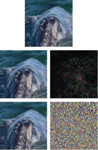
denote the decision boundaries with class 1, 2 and 3 respectively. We approximate these decision boundaries with affine hyperplanes, and the resulting decision boundary (that is the boundary of polyhedron P˜0) is shown in green. . . 23 3.6 An example of adversarial perturbations. First row: the original image x

that is classified as ˆk(x)=“whale”. Second row: the image x+r classified as ˆk(x+r)=“turtle” and the corresponding perturbation r computed by the proposed algorithm. Third row: the image classified as “turtle” and the corresponding perturbation computed by the fast gradient sign method [GSS15]. Our approach leads to a smaller perturbation. . . 27

(14)

3.7 Illustration of the quantities used in the computation of Eq. (3.17). Note that for the optimal perturbation r∗, we have g(x0+r∗) is collinear to

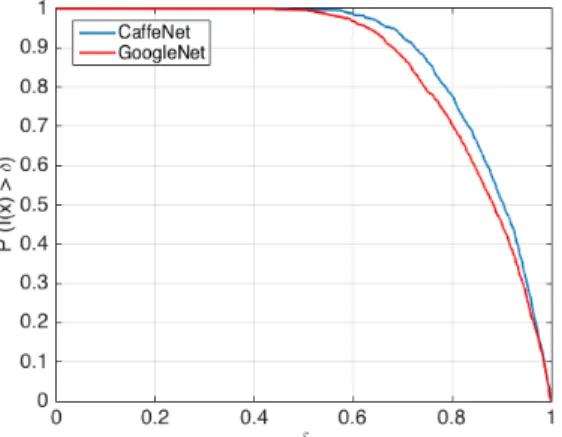
r∗. The quantity in Eq. (3.17) measures the angle between the estimated perturbation ˆr and the gradient vectorg(x0+ ˆr). . . 29 3.8 Empirical distribution ofI(x)(quantity defined in Eq. (3.17)) for a randomly

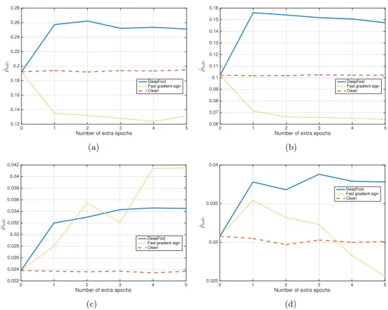
chosen population of imagesxfrom ILSVRC 2012 validation set on CaffeNet and GoogleNet. Theyaxis is the empirical probability thatI(x)> δ, and the xaxis is the threshold δ. . . 29 3.9 Effect of fine-tuning on adversarial examples computed by two different

methods for (a) LeNet on MNIST, (b) fully-connected network on MNIST, (c) NIN on CIFAR-10, (d) LeNet on CIFAR-10. The proposed method is

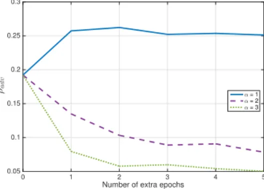
labeled as “DeepFool”. . . 30 3.10 Fine-tuning based on magnified adversarial perturbations computed using

our approach. . . 31 3.11 From “1" to “7" : original image classified as “1" and the perturbed images

(using our approach) classified as “7" using different values ofα. . . 31 3.12 How the adversarial robustness is judged by different methods. The values

are normalized by the corresponding ρˆadvs of the original network. The proposed method is labeled as “DeepFool”. . . 32

4.1 (a...e): Class 1 images. (f...j): Class -1 images. . . 36 4.2 Robustness to adversarial noise of linear and quadratic classifiers. (a):

Original image (d= 4, and a= 0.1/√d), (b,c): Minimally perturbed image that switches the estimated label of (b)flin, (c)fquad. Note that the difference between (b) and (a) is hardly perceptible, this demonstrates thatflin is not robust to adversarial noise. On the other hand images (c) and (a) are clearly different, which indicates that fquad is more robust to adversarial noise . . . 38 4.3 Adversarial robustnessρadv versus risk diagram for linear classifiers. Each

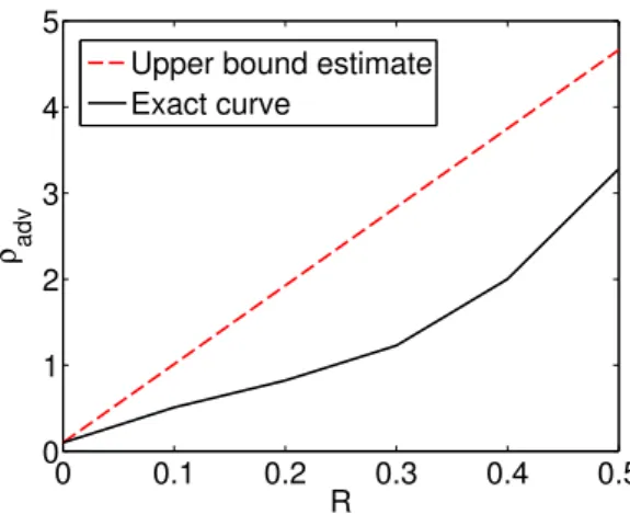
point in the plane represents a linear classifierf. The non-achievable zone is shown (Theorem 1). In the simplified case of Theorem 1, the intercept is equal to 1₂kEµ1(x)−Eµ−1(x)k2, and the slope is equal to2M. . . 42 4.4 The exact ρadv versus risk achievable curve, and our upper bound estimate

on the running example. . . 43 4.5 Original image (a) and minimally perturbed images (b-f) that switch the

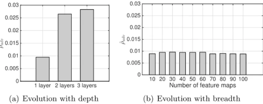
estimated label of linear (b), quadratic (c), cubic (d), RBF(1) (e), RBF(0.1) (f) classifiers. . . 46 4.6 Same as Fig. 4.5, but for the “airplane” vs. “automobile” classification task. 47 4.7 Evolution of the normalized robustness of classifiers with respect to (a) the

depth of a CNN for CIFAR-10 task, and (b) the number of feature maps. . 48 4.8 DeepCAPTCHA example. The large image is the perturbed image, and the

smaller ones are the candidate images. Image taken from [Osa+16]. . . 49

5.1 ζ1(m, δ)andζ2(m, δ)withδ= 0.05in function ofm. . . 54 5.2 Illustration of the quantities introduced for the definition of the curvature of

(15)

List of Figures

5.3 Binary classification example where the boundary is a union of two sufficiently distant spheres. In this case, the curvature isκ(Bi,j) = 1/R, whereRis the

radius of the circles. . . 56 5.4 Normal section of the boundaryBi,j with respect to planeU =span(n,u),

where nis the normal to the boundary atp, anduis an arbitrary in the tangent space _Tp(Bi,j). . . 57

5.5 (a) Original image classified as “Cauliflower”. Fooling perturbations for VGG-F network: (b) Random noise, (c) Semi-random perturbation with

m= 10, (d) Worst-case perturbation, all wrongly classified as “Artichoke”. . 62 5.6 Boundaries of three classifiers near randomly chosen samples. Axes are

normalized by the corresponding∆advsince our assumption in the theoretical bound (Corollary 1) depends on the product of∆advκ. Note the difference in range betweenxandy axes. Note also that the range of horizontal axis in (c) is much smaller than the other two, hence the illustrated boundary is more curved. . . 63 5.7 A fooling hidden message,_S consists of linear combinations of random words. 64 6.1 Schematic representation of the problem encountered by using metric theL2

metric. Black pixels indicate pixels with value0, andxτ1, xτ2 are obtained by applying a combination of rotation and translation toxτ0. Original image taken from [GBS05]. . . 68 6.2 Images along the geodesic path fromxτ0 toxτ2. Original image taken from

[GBS05]. . . 68 6.3 Schematic representation of the discretized manifold_T∗, and the Fast

March-ing update rule. In this figure, we haveN(τ) ={τ , τ˜ min, τa, τb}. . . 70

6.4 Distance map withTdil+rotgroup (left), and correctly classified regions (right), for the four tested classifiers on a “4” digit image. Details for a): the color code indicates the geodesic distance from the identity transformation (shown by red dot at the center). For each classifier, the minimal transformation for which the output of the classifier is not correct (i.e., not “4”) is indicated, along with the corresponding transformed image and geodesic path. Details for b): the region where the classifier correctly outputs the label “4” is shown in white. Geodesic paths are also shown. . . 72 6.5 Distance map with_Tdil+rotgroup (left), and correctly classified regions (right),

for the four tested classifiers on a “0” digit image. Details for a): the color code indicates the geodesic distance from the identity transformation (shown by red dot at the center). For each classifier, the minimal transformation for which the output of the classifier is not correct (i.e., not “0”) is indicated, along with the corresponding transformed image and geodesic path. Details for b): the region where the classifier correctly outputs the label “0” is shown in white. Geodesic paths are also shown. . . 73 6.6 Invariance scores of CNNs on _Ttrans, Tdil+rot and Tsim, for the CIFAR-10

(16)

6.7 Sample images from the CIFAR-10 dataset and their invariance to similarity transformations∆_T(x)(with_T =Tsim) for the NiN classifier. The odd rows show the original images, and the even rows show the minimally transformed images changing the prediction of the classifier. The invariance score ∆T(x)

is indicated on each transformed image. All original images arecorrectly classifiedby the NiN classifier. We haveρT(ˆk) = 1.15. . . 76

6.8 Sample images from the CIFAR-10 dataset and their invariance to translation

∆T(x)(withT =Ttrans) for the NiN classifier. The odd rows show the original images, and the even rows show the minimally transformed images changing the prediction of the classifier. The invariance score∆T(x)is indicated on

each transformed image. All original images are correctly classified by the NiN classifier. We have ρT(ˆk) = 1.82. . . 77

6.9 Invariance score versus number of additional training samples, for MNIST and CIFAR-10, with_T =Tsim. . . 78 6.10 Qualitative comparison between the invariance of the original NiN network

and the one trained using augmented samples, on randomly chosen samples. Images with green label represent the original images along with the correct label. The two rows below original images represent the minimally perturbed images required to modify the estimated label, respectively for the original NiN and the NiN trained with300000augmented samples. . . 79

7.1 Example map of the (un-normalized) posterior distribution pcl(τ|y(x),x) when_T =2d translations. We overlay samples obtained using the Metropolis MCMC method. . . 86

7.2 Original images are shown in row 1. Samples drawn from prior distribu-tion withα = 100 [row 2, mild transformations], α= 50[row 3, medium transformations], andα= 10 [row 4, severe transformations]. . . 88 7.3 Samples drawn from the posterior distributionp(τ|y(x),x)withα= 100. On

the left, the original image, and then the transformed images with nuisances sampled from the posterior distribution for the CNN-2 with Spatial Trans-former Network. The estimated label by the classifier of each transformed image is shown on top of each image. All shown images are misclassified by the classifier. . . 89

7.4 Transformed versions of images taken from the ILSVRC 2012 validation dataset. . . 90

7.5 Robustness of different networks trained on ImageNet to piecewise affine transformations. The left column displays original images, and the other columns show the transformed images, where transformations are sampled from the posterior pcl(τ|y(x),x) for4 different classifiers. The estimated label of each image is shown on top. A post-processing step was applied similarly to the experiment in Fig. 7.3 (see footnote 2). . . 91

(17)

List of Figures

7.6 How to transform a white wolf into (a) a polar bear, (b) an Arctic fox, (c) a Samoyed dog? For each of the three target labels, the left image represents the motion vectors of the average sampled transformations. For clarity, we overlayed on top of the motion vectors the original image classified as “white wolf”. The right image depicts the result of applying this (average) transformation to the original “white wolf” image. Experiments performed on the VGG-16 classifier. . . 92 7.7 Robustness of VGG-Faces classifier to artificial occlusion. Left column:

original image, with correct label. Columns 2 to 4 are samples from the posterior distribution. On top of each image, we indicate theestimated label. A post-processing step was applied similarly to the experiment in Fig. 7.3 (see footnote 2). . . 93 7.8 Evolution of the log-likelihoodlog(pcl(y(x)|τ,x))in one run of the Metropolis

algorithm. . . 94 7.9 Average over all nuisance samples from the posterior leading to a

misclassifi-cation, for two different images. Left: the nuisance parameters are illustrated without the original image. Right: same image, where the face image is shown in the background. . . 95

A.1 Example images in a toy classification problem where the goal is to distinguish the different balls (a: basketball, b: soccer). (c) represents an umbrella that does not belong to any class. Black pixels are equal to 0, white pixels are equal to1, grey pixels are set around0.9. . . 106 B.1 Boundingkxγ−xk2 in terms ofκ. . . 110 B.2 Left: To prove the upper bound, we consider a ball_B included in_Rk that

intersects with the boundary atx∗. Upper bounds on_krk

Sk2 derived when the boundary is ∂B are also valid upper bounds for the real boundaryBk.

Right: Normal section to the decision boundary Bk =∂B along the normal

plane _U=span rT_S,rk

. We denote byγ the normal section of boundary

Bk, along the planeU, and byTx∗B_k the tangent space to the sphere∂Bat

x∗_{. . . 113}

B.3 Left: To prove the lower bound, we consider a ball B0 _{included in} _R_ˆ

k(x0) that intersects with the boundary at x∗. Lower bounds on _krk_Sk2 derived when the boundary is the sphere ∂B0 are also valid lower bounds for the real boundary Bk. Right: Cross section of the problem along the plane

U0₌_span _rk

S,rk

. γ denotes the normal section ofBk =B0along the plane

U0_{. . . 115}

B.4 The worst-case perturbation in the subspace_S when the decision boundary is ∂B andTx∗(∂B)(denoted respectively byrB_S andrT_S) are collinear. . . 117

(18)

(19)

List of Tables

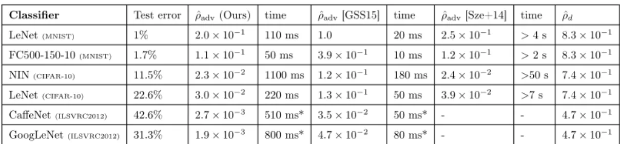
3.1 Quantities of interest and their dependencies. . . 19 3.2 The adversarial robustness of different classifiers on different datasets. The

time required to compute one sample for each method is given in the time columns. The times are computed on a Mid-2015 MacBook Pro without CUDA support. The asterisk marks determines the values computed using a GTX 750 Ti GPU. . . 26 3.3 Values of ρˆ∞_adv for four different networks based on the proposed method

(smallest `∞ perturbation) and fast gradient sign method with 90% of

misclassification. . . 28 3.4 The test error of networks after the fine-tuning on adversarial examples (after

five epochs). Each columns correspond to a different type of augmented perturbation. . . 32

4.1 Summary of quantities computed for the running example of Section 4.2, withd= 4. In blue, we show numerical values obtained witha= 0.005, for easier numerical comparison. . . 45 4.2 Training and testing accuracy of different models, and robustness to

ad-versarial noise for the MNIST task. Note that for this example, we have

ˆ

ρd = 0.72. . . 46

4.3 Training and testing accuracy of different models, and robustness to ad-versarial noise for the CIFAR task. Note that for this example, we have

ˆ

ρd = 0.39. . . 47

4.4 The parameterρˆd, and distinguishability measures for the two classification

tasks. For the numerical computation, we usedK = 1. . . 47 5.1 β(f;m)for different classifiersf and different subspace dimensions m. The

VGG-F and VGG-19 are respectively introduced in [Cha+14; SZ14]. . . 61

6.1 Accuracy and invariance scores of different classifers on the MNIST dataset. 72

7.1 Robustness to affine transformations of several networks on the MNIST dataset. Each network is trained for50epochs. . . 88 7.2 Robustness to piecewise affine transformations νˆ_T of different networks

trained on ImageNet . . . 89

(20)

(21)

1 Introduction

The goal of many computer vision tasks is to estimate categorical properties from visual data, such as the presence or absence of a particular object in a scene. For example, in the context of self-driving vehicles, one of the key tasks is to accurately recognize cars, traffic signs and pedestrians, even when these are affected by clutter, noise, occlusions and other forms of perturbation. One of the major difficulties in classification tasks is to correctly recognize an object despite the large amount of variability and corruptions that might affect the visual data in real-world tasks. While the human visual system is partially robust to such perturbations, it is unclear whether classifiers enjoy the same robustness properties. Understanding the robustness of classifiers to real-world perturbations is therefore primordial in the quest of designing effective classifiers.

In this thesis, our primary focus is the analysis and the quantification of the classifiers’ robustness to different perturbations in the data. We study a diverse set of perturbations, ranging fromadversarial noise torandom noise, as well as more structured nuisances such as geometric transformations and occlusions. These different perturbation models are likely to affect the data in a widespread set of applications. First, a classifier might be subject toadversarial attacks, where a malicious agent having (partial or full) knowledge of the classification modelminimally alters the samples so as to “fool” the classifier. For example, in person identification, an adversary would seek to minimally modify an existing photo/fingerprint to fool the classifier to be granted access in restricted areas. In such hostile environments, the robustness of classifiers against adversarial perturbations is therefore crucial. In other classification applications, the captured data might be subject torandom

noise due to the sensing process, data transmission, or any other component of the data acquisition pipeline. This noise regime is very different from the adversarial regime, as no prior knowledge on the classifier is used in the corruption process. Moreover, in computer vision applications, visual data often undergoesstructured perturbations, such as geometric transformations, illumination changes and occlusions. These structured perturbations can be seen as some sort of data corruption that act on an ideal representation of the object. In all these cases, the major challenge in classification problems is then tofactor out such corruptions or nuisances, and recover the categorical property of interest from the perturbed versions of the data.

The importance of analyzing the robustness of classifiers to different perturbations in the data (e.g., adversarial perturbations) goes well beyond the designated applications (e.g.,

(22)

security-related problems). In fact, the quantification of the amount of noise that is required to modify the estimated label of an image is crucial for understanding the concepts that are learned by the classifier. Perturbations reveal indeed the differences between the classes from the point of view of the classifier, and therefore provide important insights on the topology of the decision boundaries that separate the classes. For example, the analysis of the perturbation required to transform a (typical) “car” image into an image classified as “plane” allows us to understand the difference between these two concepts from the perspective of the classifier. While such a perturbation would typically include specific semantic objects (such as “airplane wings”) for a human observer, it is unclear whether the typical classifiers use similar cues. The analysis of the robustness properties of classifiers is therefore crucial for improving our understanding of classifiers that are often seen as black box models.

Despite the importance of robust classification, many questions pertaining to the robustness of classifiers for different perturbation models remain open. In particular, while recent works (e.g., [Sze+14]) showed that state-of-the-art classifiers are extremely unstable to adversarial perturbations, the causes of instability remain unclear. Moreover, the effect of other typical perturbations on classifiers is unknown. For example, how are state-of-the-art deep neural networks affected by random or partially random noise? We believe these problems require quantitative answers and in-depth analyses, as they determine the reliability of such classifiers in real-world environments where perturbations occur almost systematically. An even more fundamental question is whether it is actually feasible to learn robustand accurate classifiers. More generally, it is crucial to study the interplay between the accuracy of a classifier and its robustness. Finally, when images undergo

structured perturbations (such as geometric transformations), it is important toquantify

the robustness of a classifier to such transformations. While most research papers report the accuracy of the classifier on a standard split of training and testing sets, this measure says little about the robustness of this classifier to structured nuisances. Designing an appropriate measure that summarizes the robustness of a classifier to structured nuisances (such as geometric transformations, or occlusions) is therefore an important question. In particular, it permits to understand the weaknesses of classifiers with respect to real-world nuisances.

1.1 Thesis outline

The thesis is organized as follows:

In Chapter 2, we review relevant works from the literature that relate to image classification and in particular robustness and invariance properties.

In Chapter 3, we study the problem ofestimating the robustness of classifiers to adversarial perturbations. The estimation of the classifier’s robustness involves the minimization of a non-convex objective function. We propose an efficient and accurate algorithm for estimating the robustness of classifiers that is based on an iterative linearization of the classifier’s decision function. The proposed method is shown experimentally to compare favorably with respect to other methods in terms of the robustness estimation. Experimental results moreover show that augmenting the training set with adversarial examples can

(23)

1.1. Thesis outline

increase the robustness to adversarial perturbations, and act as a regularizer to improve the accuracy of the classifiers.

Next, in Chapter 4, we analyze theoretically the robustness of classifiers to adversarial perturbations. The goal of this chapter is specifically to quantify how large the robustness to adversarial perturbations can be for fixed classification families (e.g., the family of linear classifiers). To do so, we establish learning-independent upper bounds on the robustness to adversarial perturbations, and reveal the existence of a tradeoff between robustness and classification accuracy. Specifically, we show that, for common classification tasks, it isnot possible to find a classifier in the considered family that achieves both a large robustness and a large accuracy, independently of the training algorithm used to choose the classifier. We precisely quantify this tradeoff using data-dependent measures that capture the difficulty of the classification task with respect to the classifiers’ family. Our analysis moreover suggests that the lack of robustness of classifiers is due to the lack of flexibility of classifiers with regards to the difficulty of the classification task, and that the robustness increases with the flexibility of the classification model. Experimental results finally confirm the theoretical results.

In Chapter 5, we study the robustness of classifiers in a novelsemi-random noise regime, which generalizes random and adversarial noise. In the random noise regime, data points are perturbed by noise the direction of which is picked uniformly at random in the input space. The semi-random regime generalizes this model to random subspaces of arbitrary dimension, where a worst-case perturbation is sought within the subspace. We conduct a unified theoretical analysis on the robustness of classifiers in this general noise regime, and establish precise bounds on the robustness of classifiers that depend on thecurvature of the classifier’s decision boundary. Specifically, we show that the robustness of classifiers to random noise behaves as√d times the robustness to adversarial perturbations (where

ddenotes the dimension of the data) provided the curvature of the decision boundary is sufficiently small. This result highlights the blessing of dimensionality for the robustness of classifiers to random noise, as it shows that it is theoretically possible to achieve a large robustness to random noise even if the classifier is largely unstable to adversarial perturbations. Our bounds notably extend to the general semi-random regime, where we show that the robustness precisely behaves aspd_/_m_{times the distance to boundary, with}_m

the dimension of the subspace. This result shows in particular that, even whenmis chosen as a small fraction of the dimensiond, it is still possible to find small perturbations that are constrained to be in the subspace of dimensionmand that cause data misclassification. We conclude the chapter with experimental results showing that our theoretical estimates are very accurately satisfied by state-of-the-art deep neural networks on various sets of data, which suggests that the curvature of the decision boundary of such classifiers is small.

The focus of Chapter 6 is to study and quantify theinvariance of classifiers, that is, their robustness to geometric transformations of the images (e.g., translation, rotations, etc...). We propose a principled and systematic method to measure the robustness of arbitrary image classifiers to geometric transformations. Specifically, we define the invariance measure as the minimal distance between the identity transformation and a transformation that is sufficient to change the decision of the classifier. In order to define the transformation metric, the key idea is to represent the set of transformed images as an image manifold; the transformation metric is then naturally captured by the geodesic distance on the

(24)

manifold. We propose a numerical algorithm for estimating the robustness of arbitrary classifiers to low-dimensional transformation groups, which is based on the efficient Fast Marching algorithm for computing geodesic distances on manifolds. We conduct an in-depth experimental evaluation of the proposed metric and show that our method is able to quantify the gain in invariance due to the increase of the depth of a convolutional neural network, as well as the effect of data augmentation on the invariance of classifiers. The proposed tool is then used to compare different networks in terms of their invariance, and can readily be used to objectively assess the reliability of classifiers to geometric perturbations.

Finally, in Chapter 7, we generalize the idea of assessing the invariance of classifiers to arbitrary parametric nuisance factors, such as occlusions, illumination changes or complex geometric transformations. To do so, we develop a general probabilistic framework, whose outcome is two-fold: theestimation of the robustness of classifiers to arbitrary nuisances, and the efficient sampling from problematic regions in the nuisance space that potentially lead to misclassification. The latter sampling technique is used to gain insights into the “weak spots” of classifiers, as well as on the features used to distinguish between classes. We apply the proposed framework to evaluate the robustness of state-of-the-art classifiers in natural image classification and face recognition tasks, and show that these classifiers are often only mildly robust to standard nuisances, such as occlusions. The visualization of problematic samples moreover shows, for example, that a slight occlusion of specific features in a face image can cause important errors in classification. Hence, besides the possibility to measure the robustness of classifiers to standard nuisances, the proposed framework can also be used to gain further insights on the actual discriminative image features that are used in the classification process.

1.2 Summary of contributions

The main contributions of this thesis are summarized as follows:

• We propose an accurate and efficient algorithm for estimating the robustness of classifiers to adversarial perturbations.

• We analyze the robustness of classifiers to adversarial perturbations, and show the existence of learning-independent fundamental limits on the robustness of classifiers. These limits depend on the classification risk, and reveal a novel robustness-risk tradeoff.

• We show that, for classifiers with sufficiently flat decision boundaries, the robustness to random noise is larger than the robustness to adversarial noise by a factor of the square root of the data dimenstion.

• More generally, we analyze the robustness of classifiers to a noise model that interpo-lates between random noise and adversarial noise, where minimal perturbations are sought in a randomly chosen subspace. We derive precise bounds on the robustness of classifiers in this generalized noise regime in terms of the curvature of the decision boundary and the subspace dimension. We show that state-of-the-art classifiers remain vulnerable to noise that is mostly random, and only mildly adversarial (i.e., where the subspace dimension is small).

(25)

1.2. Summary of contributions

• We propose a novel invariance score that measures the robustness of a classifier to geometric transformations, and propose an algorithm for computing the invariance score.

• We finally introduce a new probabilistic framework for assessing the robustness of classifiers to parametric nuisance sets, such as occlusion or illumination changes. The proposed framework allows us to discover the “weak spots” of any given classifier using appropriate sampling strategies.

(26)

(27)

2 Prior art

2.1 Outline

In this chapter, we review the relevant works from the literature that are linked to the general problems addressed in this thesis. We first review in Section 2.2 some of the major advances in the problem of image classification, with a special emphasis on deep convolutional networks, as these have been recently shown to largely outperform other architectures. Next, in Section 2.3, we focus on the problem of robust classification. We then delve into the related problem of achieving geometric invariance to transformations and other nuisance variables in the data in Section 2.4. In this chapter, we give particular emphasis on works that analyze and provide a better understanding of the inner mechanisms of modern classification methods.

2.2 Advances in image classification

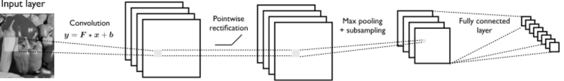
In this section, we review some of the key works in the broad domain of image classification, with a special focus on recent architectures. The main challenge for accurately solving a visual task (in particular, image classification) is building a successful visual representation, which defines a mapping from pixels to meaningful features that can be used to solve the task. Since the very beginning of computer vision, a large number of visual representations have been proposed to tackle visual tasks [Sze10]. Prior to the popularization ofdeep learning for image classification, visual representations were mostly built in ahand-engineered fashion. Examples of such representations are SIFT [Low04], HOG [DT05], SURF [Bay+08]. See [MS05] for other examples. These feature representations leverage the human expertise to define plausible mappings from the pixels to features that satisfy the required properties (such as local invariance to rotations and translation). Unlike hand-engineered representations, the modern approach builds deep visual representations by gradually transforming the image into more abstract (and more useful) representations using a number of elementary operations. Deep representations take a broad inspiration from the hierarchical nature of the architecture of the visual cortex, where visual data flows from the retina to different visual areas [TFT01]. Deep visual representations are moreover learned from the data and impose no specific priors related to the problem modality. Thanks to the rapid development of GPUs, it is now possible to learn huge deep networks (possibly containing hundreds of millions of parameters) that significantly outperform previous state-of-the-art results in

(28)

many problems, such as natural image classification (ImageNet) [KSH12; Sze+15; SZ14], face recognition [PVZ15; Tai+14], and fine-grained classification [Wah+11; JSZ+15]. Deep convolutional networks build a representation of the data through the composition of linear and nonlinear elementary operations. We briefly mention three of the key operations used in deep convolutional networks as follows:

• Convolution: Given a three-dimensional feature map x ∈ RH×W×D_{, the}

convolu-tion layer convolves x with learned filters f ∈ RH0_×_W0_×_D_×_D00

, and outputs y ∈ RH00_×_W00_×_D00 ; i.e., yi00_,j00_,d00 =b_d00+ H0 X i0=1 W0 X j0=1 D X d=1 fi0_,j0_,d,d00x_i00₊_i0₋₁_,j00₊_j0₋₁_,d,

wherebd00 denotes the bias, andH00= 1 +H−H0 andW00= 1 +W−W0.

• Rectification: Modern deep convolutional neural networks use a half-rectification activation functions defined by

y= max(0,x).

This simple nonlinearity has been shown to provide significant improvements with respect to traditional sigmoid activation functions [GBB11; MHN13], and is also tightly related to sparse coding [FDF15].

• Pooling: The goal of a pooling operation is to provide invariance to the classifier, by computing summary statistics over groups of features. Given a feature map x, the pooled representation is given by

yi00_,j00_,d=P {x_i00₊_i0₋₁_,j00₊_j0₋₁_,d}₁_≤_i0_≤_W0

1≤j0≤H0

!

,

whereW0andH0denote respectively the width and heights of the pooling regions, and

P denotes the pooling operator. Successful pooling operators include theaverage and

maximum; see e.g., [BPL10] for a comparison between different pooling mechanisms. A pooling operation is often accompanied with a subsampling of the feature map.

Input layer

Convolution

y=F?x+b

Pointwise

rectification + subsamplingMax pooling Fully connectedlayer

Figure 2.1: Structure of a CNN, obtained by stacking a series of linear and nonlinear elementary operations.

We refer to [VL15] for example for a detailed and hands-on description of other types of elementary operations commonly used in CNN architectures. The resulting classifier is a composition of many such operations, resulting in networks with possibly millions of

(29)

2.2. Advances in image classification

unknown parameters. An example architecture of a simple CNN is illustrated in Fig. 2.1. Once the architecture of the network is specified, the convolutional neural network istrained

in an end-to-end fashion using example images. Specifically, this step involves learning the convolutional filters f. Convolutional neural networks are generally trained using stochastic gradient descent (SGD) optimization, where the chain rule – or backpropagation [LeC+98b] – is used in order to compute the gradients. Alternative optimization algorithms have however been proposed recently, and have been shown to improve over standard optimization algorithms [KB14; MG15; Mar10].

Figure 2.2: Images obtained using the visualization tool of [SVZ13] where the “goose” and “ostrich” neurons in the last layer of a deep neural network are maximized. Image taken from [SVZ13].

The recent impressive success of deep convolutional neural networks has triggered a signifi-cant number of fundamental research questions related to our understanding of the internal mechanisms leading to these successes. In an attempt to understand the features learned by deep networks, visualization strategies have been proposed in [MV15; DB16]. These visualization tools study the invertibility of the CNN representations; that is, to which extent an imagexcan be recovered from its feature representationφ(x)? The visualization of these inverse images gives an understanding of the information that is preserved in the feature representations. In particular, these visualization strategies provide some empirical understanding about the layers at which invariance in the representation is achieved. Other visualization tools have been proposed in [ZF14; SVZ13], where the authors focus instead on the visualization of images that maximize the activation of single neurons. Fig. 2.2 shows images obtained by maximizing class-specific neurons in a state-of-the-art deep neural network. Experiments with these visualization tools show that, while neurons in lower layers mostly fire in the presence of edges, neurons in higher layers tend to be more sensitive to semantic objects with similar visual appearance. The invertibility of convolutional networks has also been studied from a theoretical perspective. In [BSL14], the invertibility of pooling operations used in neural network representations is analyzed. In particular, it is shown that, when the linear weights of the neural network are sufficiently redundant, it is possible to recover the original signals from pooled representations. Along the same lines, [ALM15] show that neural nets have an associated simple generative model that generates input data according to the conditional distribution characterizing the neural network.

Since the elementary operations that constitute convolutional neural networks are all linear or piecewise linear, the associated feature mapping is globally piecewise linear in

(30)

the image space. In [Mon+14], the number of linear regions (in the input space) of deep neural networks is studied; this number is shown to grow exponentially with the number of layers and polynomially in the size of the hidden layer. This growth therefore highlights that deep networks are more flexible than shallow ones, and hence can compute more “complicated” functions, which partly explains their success. Along the same lines of a theoretical understanding of the effect of deep networks on the input space, the authors in [ABB15] study the effect of applying half-rectification non-linearities on the input space, and in particular, on the linear separability of the datapoints.

On the optimization front, several works have attempted to understand the landscape of the non-convex objective function used to train deep neural networks [Dau+14; Cho+14]. In [Dau+14], the authors show that the difficulty in training such neural networks comes from the abundance of saddle points, not local minima, particularly in high dimensional problems that we typically encounter in neural network training. The authors empirically show that such saddle points are surrounded by high error plateaus that can make learning more difficult. In [Cho+14], the authors provide a theoretical description of the optimization of large neural networks, under strong statistical assumptions on the network. It is shown in particular that, under such assumptions, most local minima of the objective function are equivalent in the sense that they yield similar performance on a test set. The probability of finding a bad local minima (i.e., large objective function) is further shown to decrease with the network size; i.e., while for small-sized networks, “bad” local minimas have a non-zero probability of being recovered, the probability of recovering such local minimas for large networks is actually very small. Despite the strong statistical assumptions imposed on the network, this work provides a better understanding of the shape of the objective function, and explain why it is possible to train very deep networks using simple algorithms such as stochastic gradient descent.

One of the main goals of this thesis is to develop analytical results in order to increase our understanding of classification models, and in particular, the robustness of classifiers to perturbations in the data. In the following sections, we review recent works related to the robustness of classifiers to different perturbation models.

2.3 Classification robustness

Robustness of neural networks to adversarial perturbations

State-of-the-art deep neural networks have recently been shown to be unstable toadversarial perturbations in the data [Sze+14]. Unlike random noise, adversarial perturbations are

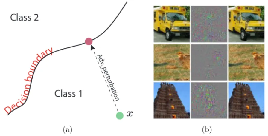
minimal (or worst-case) perturbations that are sought to change the estimated label of the classifier. The computation of adversarial perturbations involves solving an optimization problem (that requires the knowledge of the classifier’s model), with the goal of going beyond decision boundary of the classifier (see Fig. 2.3 (a) for an illustration). On vision tasks, the results of [Sze+14] have shown that perturbations that are hardly perceptible to the human eye are sufficient to change the decision value of a deep network, even if the classifier has a performance that is close to the human visual system (Fig. 2.3 (b)). This surprising instability to “invisible” perturbations has received a widespread interest, as it highlights a fundamental difference with the human visual system, and raises important

(31)

2.3. Classification robustness challenges. Adv . per tur ba tion

De

cis

io

n

bo

un

da

ry

x

Class 1

Class 2

(a) (b)

Figure 2.3: Illustration of adversarial perturbations. Left: schematic representation of the perturbation. Right: Example images and adversarial perturbations. The left column depict original images (correctly classified by the network), the middle column shows the perturbations, and the right column shows the perturbed images (original image + perturbation) that are wrongly classified. This figure is taken from [Sze+14].

Beyond the obvious security concerns that this instability issue raises when classifiers are deployed in hostile environments, it also reveals fundamental shortcomings in the concepts and decision boundaries learned by state-of-the art classifiers. Specifically, this instability shows that most datapoints lie very closely to decision boundaries, even for two classes with significantly different semantic meaning. It should be noted that the authors in [Sze+14] have previously imputed the high instability of deep neural networks to the high “nonlinearity” of these classifiers. More precisely, the large Lipschitz constants associated to the feature map of the CNN are thought to induce “blind spots” in the classifier causing the instability to small perturbations. This explanation does not, however, take into account the important fact that linear classifiers are not exempt from this instability to adversarial perturbations. In that context, one of the contributions of this thesis is to provide a quantitative analysis of the robustness of classifiers to adversarial perturbations, with the goal of gaining a better understanding of this phenomenon.

While in [Sze+14], it is assumed that the adversary has full knowledge of the classification model, other works have examined the robustness of classifiers to perturbations when the adversary has only limited knowledge [Big+13; DSX10; GR06]. For example, in [Big+13], the transformed data point is constrained to remain within a maximum distance from the original sample, and it is further assumed that the attacker does not have direct access to the model (but only to a surrogate). These attack models are more likely to occur in real-world applications, as attackers often do not have complete control over the classification model.

Construction of robust classifiers with robust optimization

Following the original paper [Sze+14], several attempts have been made to construct deep networks with better robustness to adversarial perturbations [CPE14; GR14]. While most of these recent works that attempt to construct robust classifiers have mostly focused on the robustness of the new generation of neural networks to perturbations in the data, the

(32)

design of robust classifiers has been an active area of research and a long standing goal in machine learning. Using a robust optimization approach, new learning algorithms have been proposed for various learning tasks (see [CMX12] and references therein). A particular emphasis was given to the extension of support vector machines (SVMs) to settings where uncertainty corrupts the data. Assuming a disturbance model on the data samples, the robust optimization approach for constructing robust classifiers seeks to minimize the worst possible empirical error under such disturbances. In the context of SVM classification, the problem of learning robust linear classifiers(w, b)corresponds to the following min-max problem min w,b maxU∈U ( r(w, b) + m X i=1 1−yi((xi+ui)Tw+b)₊ ) ,

wherexianduidenote respectively the datapoints and perturbation vectors,yi∈ {+1,−1}

denote the labels and r(w, b)is a regularization term. For certain uncertainty sets_U, the objective function can be written as a tractable convex optimization problem [XCM09; Lan+03; Bha04; TG07], which makes the task of finding a robust classifier feasible.

Other works have applied robust optimization approaches to design robust classifiers against new forms of perturbation. For example, in [GR06; DSX10], the authors propose a robust optimization algorithm to train classifiers that are robust against missing features (e.g., missing pixels in a handwritten recognition task). In [CM08], the problem of robust classification is examined when the noise affects the labels rather than the datapoints; it is then shown that robust classifiers can also be trained using robust optimization.

Unlike the above works that mostly propose robust classification algorithms for SVM, we focus in this thesis on more analytical aspects; e.g.,can we actually find classifiers that are robust to perturbations? Moreover, we mostly concentrate in this thesis on modern successful architectures (e.g., deep neural networks) that have achieved huge progress in the problem of image classification. It should be noted that the construction of robust classification methods for deep neural networks is still an open problem.

Robustness at the learning stage

While most of the above works consider attacks that alter datapoints at test time, it is equally important to achieve robustness to perturbations at thetrainingstage. In particular, the adversary might manipulate the training data, therefore leading to a modification of the learned classification rule. This type of attack, dubbedpoisoning attack, injects specially crafted training samples in order to maximize the test error of the learned classifier. The effect of poisoning attacks on different learning algorithms have previously been investigated in [BNL12; Xia+15]. In [Bar+06; Dal+04], a taxonomy of different attacks at the training stage requiring different levels of knowledge about the machine learning systems, and methods to counter these attacks are described. It is important to stress that, while these works study attacks that manipulatethe learning system (e.g., change the decision function by injecting malicious training points), as well as defense strategies to counter these attacks, our focus in this thesis is more on robustness of fixed classifiers (not the learning algorithms). We finally note that the stability of learning algorithms has also been defined and studied

(33)

2.4. Classification invariance to geometric transformation and nuisance factors in [BE02; LP94a]. Specifically, in [BE02], the stability of learning algorithms is examined with respect to a removal of an element in the training set; this notion of stability is further shown to be useful in order to derive generalization error bounds. This is again a property of the learning algorithm; we are however more interested in this thesis on the robustness of fixed classifiers.

2.4 Classification invariance to geometric transformation and

nuisance factors

In visual tasks, it is not only crucial to have classifiers that are robust against additive or adversarial attacks; it is also equally important to achieve invariance to structured nuisance variables, such as illumination changes, occlusions or standard local geometric transforma-tions of the image. Specifically, when images undergo such structured deformatransforma-tions, it is desirable that the estimated label remains the same. In this part, we will first review some of the works that impose invariance by modifying the distance measure or by appropriate alignment. Then, we will review modern techniques that implicitly incorporate invariance in deep feature representation. Finally, we will review the relevant works in the literature thatassess and analyze the invariance of classifiers to nuisance factors.

Transformation invariant distances and image alignment

One approach to introduce invariance in pattern recognition algorithms is to use transformation-invariantdistance measures. The geometrically transformed versions of a fixed image span a low-dimensional nonlinear manifold in the high-dimensional space. Therefore, an appropriate invariant distance measure in this case corresponds to the manifold distance between these two transformation manifolds. Computing the transformation-invariant distance between two patterns or, equivalently, the manifold distance is unfortunately a difficult problem in general. The authors in [Sim+00] locally approximate the transformation-invariant distance with the distance between the linear spaces that are tangent to both manifolds. [VL05] go beyond the limitations of local invariance in tangent distance methods by embedding the tangent distance computation in a multiresolution framework. In [KF09], global invariance is achieved by approximating the original pattern with a linear combination of atoms from a parametric dictionary. Thanks to this approximation, the manifold is given in a closed form, and the objective function becomes equal to a difference of convex functions that can be globally minimized using cutting plane methods. Unfortunately, this class of optimization methods has a slow convergence rate with complexity limitations in practical settings.

Another approach for computing the transformation-invariant distance is to align (or

register) the images. Transformation-invariant distances can then be easily computed from the aligned versions of the image. Feature-based approaches [Low04; DT05; Bay+08] represent an efficient class of methods for image registration. They are usually built on several steps: (i) feature detection, which searches for stable distinctive locations in the images, (ii)feature description, which provides a description of each detected location with an invariant descriptor, (iii)features matching between the images and (iv)transformation estimation that estimates the global transformation by looking at matched features. Note that it is crucial in this class of methods to describe the features in a

(34)

transformation-invariant way for easier matching. Many other approaches for image alignment exist [Pen+10; Mae+97; Ash07; FF13]; a comprehensive review of these approaches however goes outside the scope of this thesis, and we refer to [ZF03; Sze10] for surveys on this topic.

Invariant feature representations

Deep convolutional networks build features that intend to be invariant to local geometric deformations in the data, through the use of a cascade of convolution, pooling and nonlin-earity operators as discussed earlier in this chapter [Jar+09]. Despite the success of these architectures, their invariance properties are not fully understood. What is the effect of the number of layers on the invariance of the architecture? Which nonlinearity and pooling operations to use in order to enhance the invariance of the global representation? In [Mal12; BM13], the authors use a similar structure to convolutional neural networks (i.e., cascade of filtering, nonlinearity and pooling operations), and imposethe requirement of stability of the representation to local deformations, while retaining maximum information about the original data. Formally, the feature mapping Φis imposed to satisfy the following stability conditions:

Stability to additive noise: _kΦk ≤Ckk, (2.1) Stability to local deformations: _kΦxτ −Φxk ≤Ckxksupu|∇τ(u)|, (2.2)

whereτ(u)is a displacement field that deforms the image,xτ(u) =x(u−τ(u)), and| · |

is the matrix operator norm. It should be noted that the condition in Eq. (2.2) implies the invariance of the feature representation to global translations (i.e., special case where

∇τ(u) = 0). In order to satisfy these constraints, a new architecture is proposed, the

scattering network, where successive filtering with wavelets and pointwise nonlinearities are applied. It should be noted that the approach used to build this scattering network significantly differs from traditional convolutional neural networks, as no learning of the filters is involved. Scattering networks have been shown to achieve very high classification accuracies on digit and texture classification tasks in [BM13; SM13]. Scattering networks have also been applied to more complex tasks, such as natural image classification in [OM15]. While yielding better results with respect to previously known unsupervised dictionary learning methods and fixed-feature classification methods, scattering networks still underperform supervised CNNs in terms of classification accuracy on these complex tasks. In another effort to improve the invariance properties of deep convolutional neural networks, the authors in [JSZ+15] proposed a new module, the spatial transformer, thatgeometrically

transforms the filter maps. Spatial transformer modules, similarly to convolutional modules, are trained in a supervised way; in particular, the estimation of the transformation is performed in order to maximize the classification accuracy. Using spatial transformer networks, the performance of classifiers improve significantly, especially when images have noise and clutter, as these modules automatically learn to localize and unwarp corrupted images. Finally, another popular way of building more invariant representations is through virtual jittering (or data augmentation), where training data are transformed and fed back to the training set. One of the drawbacks of this approach is however that the training can become intractable, as the size of the training set becomes substantially larger than the original data set. To make the training more efficient with the augmented training sets, new techniques have been proposed based on the non-uniform sampling of the training data

(35)

2.4. Classification invariance to geometric transformation and nuisance factors [CJF16]. Besides, some works [Pau+14; Hau+16] have recently developed principled and automatic approaches for transforming images. Despite these major advances in building more robust and invariant representations, a thorough understanding and assessment of the invariance to general nuisance factors of these classifiers remains open.

Analyzing the invariance of classifiers

We review in this section works that assess and analyze the invariance of classifiers to transformations in the data. Several empirical works have been introduced to assess the invariance of classifiers to geometric transformations in the data. In [Goo+09], the authors develop simple tests to assess the invariance of neural networks to transformations of the data. These tests consider controlled images of gratings, and measure the effect of applying simple geometric transformations to the probe image. In a more recent work, [LV15] study theequivariance property of image representations, that is the relation between the features of the transformed images and those of the original image. The invariance is a special case of equivariance where transformation has no effect. These experiments help understanding at which layer invariance to simple transformations such as vertical flips, scale or rotation is achieved. In [Bak+16], the view-point invariance of CNNs is analyzed. In particular, the authors study the evolution of the view-manifold (that contain the features of the different views of an object) with respect to the number of layers. It is shown that the information on the view of an object is preserved till the last but one layer of the CNN. In other words, CNNs preserve the structure of the view manifold, which supports the hypothesis that this manifold in higher layers is “untangled” in higher layers, rather than being “collapsed”, which goes in the same direction of [DC07] for the human brain. In [KDS16], an empirical analysis of the ability of current CNNs to manage location and scale variability is performed. It is shown in particular that CNNs are not very effective in factoring out location and scale variability, despite the popular belief that the convolutional architecture and the local spatial pooling provides invariance to such representations.

In [SC16; SDK15; ARP16], a more theoretical perspective is taken to analyze the invariance of modern classification methods to nuisance variables. Specifically, in [SC16], the authors propose a new mathematical formalism of visual representations, and define the notion ofoptimal representation. The optimality of a representation essentially formalizes the intuitive definition of a representation that satisfies the property of invariance to nuisance variables, and retaining maximal information of the original images. Connections with existing representations (shallow and deep) are further shown. This work has suggested well-grounded modifications of existing architectures that led to significant improvements in the problem of feature correspondence in single-view and multi-view settings [DS15; Don+15].

Despite the importance of the invariance property of classifiers to nuisance variables, there exists no systematic method to test the invariance of classifiers to arbitrary nuisance variables in the data, up to our knowledge. We provide in this thesis tools toquantify the invariance of black-box classifiers to arbitrary nuisance variables.