Essays on Earnings Predictability

ESSAYS ON

EARNINGS

PREDICTABILITY

Mark Bruun

The PhD School of LIMAC PhD Series 12.2016

ESSA

YS ON EARNINGS PREDICT

ABILITY

COPENHAGEN BUSINESS SCHOOL

SOLBJERG PLADS 3 DK-2000 FREDERIKSBERG DANMARK WWW.CBS.DK ISSN 0906-6934 Print ISBN: 978-87-93339-88-0 Online ISBN: 978-87-93339-89-7

Essays on Earnings Predictability

Mark Bruun

Mark Bruun

Essays on Earnings Predictability

1st edition 2016 PhD Series 12.2016 © Mark Bruun ISSN 0906-6934 Print ISBN: 978-87-93339-88-0 Online ISBN: 978-87-93339-89-7

LIMAC PhD School is a cross disciplinary PhD School connected to research communities within the areas of Languages, Law, Informatics, Operations Management, Accounting, Communication and Cultural Studies.

All rights reserved.

No parts of this book may be reproduced or transmitted in any form or by any means, electronic or mechanical, including photocopying, recording, or by any information

Preface

Thanks to my supervisors Thomas Plenborg, Kim Pettersson, Ole Sørensen and Jesper Banghøj. Furthermore thanks to Per Olsson and Jeppe Christoffersen for acting as my discussants at my final WIP seminar and for the useful comments. Also, thanks to Hans Frimor, Peter Ove Christensen and Jan Marton for providing useful comments. Thanks to Wayne Landsman for helping me make my messages in the articles clearer as well as for useful comments. Thanks to my colleagues at the Department of Accounting and Auditing at Copenhagen Business School.

Thanks to Poul og Erna Sehested Hansens Fond and Oticon Fonden for providing the financing for my stay at University of North Carolina (Kenan-Flagler Business School).

Finally, thanks to my friends and family for moral support and their patience through the whole process. Thank you, especially Ragnhild E. Gundersen for taking care of me and our daughter Cornelia.

Summary

This dissertation addresses the prediction of corporate earnings. The thesis aims to examine whether the degree of precision in earnings forecasts can be increased by basing them on historical financial ratios. Furthermore, the intent of the disser-tation is to analyze whether accounting standards affect the accuracy of analysts’ earnings forecasts. Finally, the objective of the dissertation is to investigate how the stock market is affected by the accuracy of corporate earnings projections.

The dissertation contributes to a deeper understanding of these issues. First, it is shown how earnings forecasts can be generated based on historical timeseries patterns of financial ratios. This is done by modeling the return on equity and the growth-rate in equity as two separate but correlated timeseries processes which converge to a long-term, constant level. Empirical results suggest that these earn-ings forecasts are not more accurate than the simpler forecasts based on a histori-cal timeseries of earnings. Secondly, the dissertation shows how accounting stan-dards affect analysts’ earnings predictions. Accounting conservatism contributes to a more volatile earnings process, which lowers the accuracy of analysts’ earn-ings forecasts. Furthermore, the dissertation shows how the stock market’s re-action to the disclosure of information about corporate earnings depends on how well corporate earnings can be predicted. The dissertation indicates that the stock market’s reaction to the disclosure of earnings information is stronger for firms whose earnings can be predicted with higher accuracy than it is for firms whose earnings can not be predicted with the same degree of accuracy.

Resum´e (Summary in Danish)

Denne afhandling omhandler forudsigelse af virksomheders indkomst. Afhan-dlingen har til form˚al at undersøge, hvorvidt graden af præcision i indkomst-prognoser for virksomheder kan øges ved at basere indkomst-indkomst-prognoser p˚a his-toriske, finansielle nøgletal. Ydermere, er hensigten med afhandlingen at analy-sere hvorvidt regnskabsstandarder p˚avirker nøjagtigheden i analytikeres forudsig-elser om virksomheders indkomst. Endelig, er m˚alet med afhandlingen at un-dersøge, hvordan aktiemarkedet p˚avirkes af præcisionen i indkomst-prognoser for virksomheder.

Afhandlingen bidrager til en dybere indsigt i disse problemstillinger. For det første, vises hvordan indkomst-prognoser kan genereres udfra historiske tidsserie-mønstre for finansielle nøgletal. Dette gøres ved at modellere egenkapitalsforrent-ningen og vækstraten i egenkapitalen, som to seperate, men korrelerede tidsserie processer, som konvergerer mod et langtsigtet, konstant niveau. Empiriske re-sultater antyder, at disse indkomst prognoser ikke er mere nøjagtige end simplere prognoser baseret p˚a historiske tidsserier for indkomst. For det andet, viser afhan-dlingen, hvordan regnskabsstandarder p˚avirker analytikeres indkomst forudsigel-ser. Regnskabsmæssig konservatisme bidrager til en mere volatil indkomstproces, hvilket sænker nøjagtigheden i analytikeres indkomst-prognoser. Desuden viser afhandlingen, hvordan aktiemarkedets reaktion p˚a offentliggørelse af information om virksomheders indkomst, afhænger af i hvilken grad af præcision virksomhed-ers indkomst kan predikteres. Afhandlingen indikerer, at aktiemarkedets reak-tion p˚a offentliggørelse af indkomst-informareak-tion, er kraftigere for virksomheder hvis indkomst kan forudsiges med højere nøjagtighed, sammenlignet med virk-somheder hvis indkomst ikke kan forudsiges med samme grad af nøjagtighed.

Contents

1 Research objective 11

2 Contributions 15

3 Data and research methods 17

4 Limitations and future research 18

5 Articles 21

5.1 Using Time-series Properties of Financial Ratios to Forecast Earnings . . . . 21 5.2 Conservatism and Analysts’ Earnings Forecast Accuracy . . . 63 5.3 Earnings Predictability and the Earnings Response Coefficient . . . 113

1 Research objective

For decades, the accounting literature (starting with Ball and Brown (1968) and Beaver (1968)) has studied whether earnings announcements are relevant or in-formative to investors, by looking at how prices (or market transactions) change when earnings are announced. The informativeness of earnings announcements is important for the stock market because it enhances the efficiency of capital al-location across firms in society. The informativeness of earnings announcements is closely related to the accuracy of earnings forecasting (which is also known as earnings predictability). If earnings were perfectly predictable, earnings an-nouncements should not create a stock price movement, because there would be no earnings surprises (i.e. no new information content in the earnings). Likewise, stock price movements should only emerge because of the time value of money (i.e. less discounting of earnings)1_{. Earlier studies disagree about whether more} accurate earnings forecasting increases or decreases the informativeness of earn-ings announcements.

Another branch of the literature has studied how accurate earnings forecasts are. Lacina et al. (2011) and Bradshaw et al. (2012) compare analysts’ forecasts to time-series based earnings forecasts. They find that analyst forecasts are only superior to a simple Random Walk (RW) time-series model in the short-run (i.e. one or two years ahead). Bansal et al. (2012) and Ball et al. (2014) focus on how the short-run accuracy of time-series based earnings forecasts can be enhanced. In the same way as informativeness in earnings announcements is important for the stock market, so are accurate earnings forecasts, because earnings forecasts implicitly determine the capital allocation across firms. However, as far as my

knowledge extends, no studies have focused on enhancing the forecasting ac-curacy of long-term (i.e. four or more years ahead), time-series-based earnings forecasting.

Another way to enhance the accuracy of earnings forecasts is to change the def-inition of earnings. Changing accounting standards is a way of redefining the definition of earnings. Mensah et al. (2004), Pae and Thornton (2010) and Sohn (2012) study how accounting standards (e.g. accounting conservatism) affects the accuracy of analysts’ earnings forecasts. These studies assume that earnings volatility is exogenous. However, accounting conservatism probably changes the time-series properties of earnings, which again will affect the accuracy of ana-lysts’ earnings forecasts. Thus, earnings volatility should be treated as an en-dogenous variable.

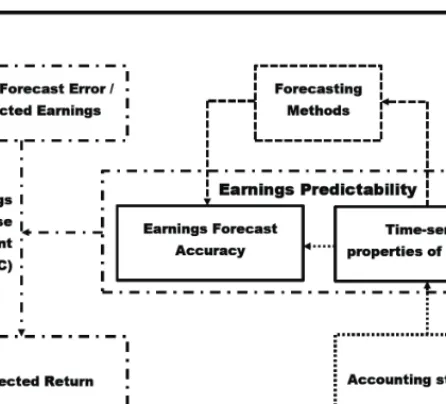
The aim of this dissertation is to provide insight into how earnings predictability (i.e. forecast accuracy) can be enhanced and how this affects the market’s reaction to earnings announcements. More specifically, the aim is to develop time-series based earnings forecasts that are more accurate than the existing time-series based earnings forecasting models; to analyze how accounting standards affect earnings predictability; and to analyze how earnings predictability moderates the relation between unexpected earnings and unexpected returns (also known as the Earnings Response Coefficient).

Figure 1: Article overview

The central concept of the dissertation, earnings predictability, is measured in different ways in the literature. The most widely used measure is the standard deviation of unexpected earnings, where unexpected earnings are defined as the forecast error (realized minus forecast value). For each firm, this measure can be estimated both cross-sectionally (i.e. based on analysts’ forecasts)2_{and based} on the time-series of earnings. The time-series properties of earnings (e.g. earn-ings volatility and persistence) is very closely related to the time-series standard deviation of unexpected earnings (Dichev and Tang (2009)). Thus, even though

2_{The standard deviation of unexpected earnings can also be estimated cross-sectionally based on time-series}

mod-els. However this requires different time-series models, since a time-series model only generates a single forecast for each firm at a given point in time.

earnings volatility and persistence do not convey any information about forecast-ing accuracy (since no forecastforecast-ing is required to estimate the earnforecast-ings volatility and persistence), they can still be used as measures of earnings predictability.

In Article 1, I study whether the accuracy of time-series based earnings forecast can be enhanced by incorporating a well-known empirical long-run time-series property of earnings as well as well-known time-series properties of financial ra-tios: namely, the long-run growth in earnings and the mean-reversion in financial ratios. By modeling Return On Equity (ROE) and growth in book value of eq-uity as two separate (but correlated) AR1 processes, I develop a time-series based model that generates mean-reversion forecasts for these financial ratios as well as forecasts where earnings grow in the long-run. Since this model incorporates well known empirical time-series properties, I hypothesize that its forecasting ac-curacy is better than that of the Random Walk (which does not incorporate long-run growth and mean-reversion of financial ratios in forecasts) and the Random Walk with drift (that does not incorporate mean-reversion of financial ratios in forecasts).

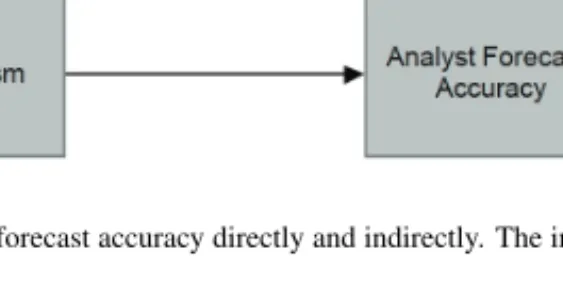
In Article 2, I study how accounting standards (e.g. accounting conservatism) affects the time-series properties of earnings and how this change in time-series properties affects the accuracy of analysts’ earnings forecasts. Using the Penman and Zhang (2002) C-score (the estimated reserve) as a measure of accounting conservatism, I study how conservatism affects the accuracy of analysts’ earnings forecasts, both directly and indirectly. The indirect effect is mediated through earnings volatility, because accounting conservatism decreases the match between revenue and expenses. This increases the volatility of earnings, which decreases the accuracy of analysts’ forecasts (i.e. makes it more difficult to forecast). Thus,

in contrast to earlier research (Mensah et al. (2004), Pae and Thornton (2010) and Sohn (2012)) that treats earnings volatility as exogenous, I treat it as an endoge-nous variable.

In Article 3, I study how earnings predictability moderates the relation between unexpected earnings and unexpected returns (also known as the Earnings Re-sponse Coefficient (ERC)). I show how the most common empirical measures of earnings predictability are related, and how earnings predictability moderates the ERC without assuming a specific earnings expectation model, in contrast to earlier research that assumes specific earnings expectation models. Furthermore, using both a market based and two time-series based measures of earnings pre-dictability, I estimate the relation between earnings predictability and the ERC.

2 Contributions

The three articles’ abstracts are replicated below.

Article 1: Using Time-series Properties of Financial Ratios to

Forecast Earnings

I forecast earnings from a model based on the time-series properties of financial ratios. This model captures two empirical patterns: mean reversion in financial ratios as well as long-run growth in earnings. I compare the accuracy of these earnings forecasts with the forecasts from a Random Walk model and analysts’ forecasts based on a sample from 2001–2013. An analysis of the accuracy shows that the earnings forecast from the financial ratio based model are closer to having an equal frequency of optimistic and pessimistic forecasts than are those from the

Random Walk. However, in terms of forecasting accuracy and mean bias, the Random Walk model is the superior model.

Article 2: Conservatism and Analysts’ Earnings Forecast

Accu-racy

Based on US data, I study the total effect that accounting conservatism has on the accuracy of analysts’ earnings forecasts. I hypothesize that conservatism af-fects this accuracy directly and indirectly via the effect that conservatism has on the time-series properties of earnings. The results show that conservatism indi-rectly and positively affects the absolute forecast errors and dispersion, because conservatism increases earnings volatility. Furthermore, the results show that con-servatism directly and positively influences the absolute forecast errors and dis-persion, which indicates that either analysts do not correctly incorporate conser-vatism into their forecasts or there are other factors (besides earnings volatility) that mediate the relation between accounting conservatism and the accuracy of analysts’ earnings forecasts. The findings suggest that regulators should not only consider the benefits of accounting conservatism, namely, protecting investors from future losses, but also the costs, in the form of higher earnings volatility and lower accuracy of earnings forecasts.

Article 3: Earnings Predictability and the Earnings Response

Coefficient

One way to measure the informativeness of accounting information is the rela-tion between unexpected stock returns and unexpected earnings (the Earnings Response Coefficient (ERC)). This paper analyzes how earnings predictability

affects the ERC. Earlier literature finds contradictory results about the relation between earnings predictability and the ERC, which might be explained by the earnings expectation model. I use three different measures of earnings predictabil-ity (earnings persistence, earnings volatilpredictabil-ity, and analyst forecast dispersion) and analytically show how they are related to each other and the ERC (without as-suming a specific earnings expectation model). The analysis reveals that higher earnings volatility is associated with a higher analyst earnings forecast dispersion and lower earnings persistence. I provide evidence that a higher ERC is associated with a higher earnings predictability.

3 Data and research methods

The data used in the articles are all from large databases: Compustat, I/B/E/S and CRSP. The earnings forecasting accuracy (i.e. earnings predictability) measure in Article 1 is based on the “Street” earnings definition in the I/B/E/S database. The definition of “Street” earnings is a definition (used by financial analysts) that gen-erally excludes nonrecurring items (Gu and Chen (2004), Abarbanell and Lehavy (2007)). I estimate the time-series model and study how earnings forecasting ac-curacy differs across this model, the Random Walk model and analyst forecasts. Estimation of the time-series properties on the individual firm-level implies small estimation samples. Under the assumption that the estimates of the time-series properties are consistent, increasing the sample size increases the probability of the estimates’ being close to the true value. To increase the sample size, I estimate the time-series properties of financial ratios grouped by industry, based on panel data. This, however, comes with a cost in terms of assuming that the time-series properties of the financial ratios are homogeneous across firms within an industry.

In Article 2, information from Compustat is used to estimate the conservative accounting factor (estimated reserve) as well as the earnings volatility and the I/B/E/S database is used to calculate the accuracy of analysts’ forecasts (i.e. earn-ings predictability). The hypotheses in Article 2 were tested via path analysis using the PROC CALIS procedure in SAS.

In Article 3, the Earnings Response Coefficient (ERC) is estimated in the usual way (the ERC is the parameter estimate from regressing unexpected earnings on unexpected returns). The unexpected returns are estimated using stock re-turns from CRSP and the market model. The unexpected earnings are estimated from the I/B/E/S database as the difference between analysts’ earnings forecasts and realized earnings. Estimating the earnings volatility and the earnings persis-tence (i.e. measures of earnings predictability) requires longitudinal data. There-fore I estimate the earnings volatility and earnings persistence based on earnings from Compustat, since estimating the earnings volatility and persistence from the I/B/E/S data would reduce the sample size significantly. Even though the defini-tions of earnings in I/B/E/S and Compustat differ, these measure are very probably highly correlated.

I test the hypotheses in Article 3 in the two step approach proposed by Cready et al. (2001): first I estimate individual firm ERCs; second, I regress the ERCs on earnings predictability and the market-to-book ratio.

4 Limitations and future research

Regarding Article 1, it is likely that the forecasting performance could have been enhanced by disaggregation of the (scaled) earnings into cash flow and

accru-als, since cash flows are more persistent than accruals (Sloan (1996)). Another possible disaggregation that might enhance the forecasting accuracy is splitting earnings into operating earnings and financial earnings. Thus, future research could study whether disaggregation can increase the forecasting accuracy of the proposed time-series model.

Article 2 only focuses on accounting conservatism from the cost side (i.e. ex-pensing vs. capitalizing R&D and advertising costs). However, accounting con-servatism can also arise on the revenue side by the choice of revenue recognition methods (i.e. completed-contract vs. percentage-of-completion method). Hence, a natural extension is to focus on unconditional conservatism from the revenue side.

In relation to Article 3, earlier studies (Sadka and Sadka (2009), Patatoukas (2014)) have made suggestions as to why the Earnings Response Coefficient (ERC) is neg-ative when focusing on the aggregated level. Article 3 only focuses on the relation between earnings predictability and the ERC at the individual firm level. How-ever, since the sign of the ERC is different depending on whether one looks at the individual firm level or the aggregated level, it is likely that the relation between earnings predictability and the ERC also depends on whether the focus is on the individual firm level or the aggregated level.

References

Abarbanell, J. S. and R. Lehavy (2007). Letting the ”tail wag the dog”: The debate over gaap versus street earnings revisited. Contemporary Accounting Research 24, 675–723.

Ball, R. and P. Brown (1968). An empirical evaluation of accounting income numbers. Journal of Accounting Research 6, 159–178.

Ball, R., E. Ghysels, and H. Zhou (2014). Can we automate earnings forecasts and beat analysts? Working paper.

Bansal, N., J. Strauss, and A. Nasseh (2012). Can we consistently forecast a firms earnings? using combination forecast methods to predict the eps of dow firms.

Journal of Economics and Finance.

Beaver, W. H. (1968). The information content of annual earnings announce-ments. Journal of Accounting Research 6, 67–92.

Bradshaw, M. T., M. S. Drake, J. N. Myers, and L. A. Myers (2012). A re-examination of analysts’ superiority over time-series forecasts of annual earn-ings. Review of Accounting Studies 17, 944–968.

Cready, W. M., D. N. Hurtt, and J. A. Seida (2001). Applying reverse regres-sion techniques in earningsreturn analyses. Journal of Accounting and Eco-nomics 30, 227–240.

Dichev, I. D. and V. W. Tang (2009). Earnings volatility and earnings predictabil-ity.Journal of Accounting and Economics 47, 160–181.

Gu, Z. and T. Chen (2004). Analysts treatment of nonrecurring items in street earnings.Journal of Accounting and Economics 38, 129–170.

Lacina, M., B. B. Lee, and R. Z. Xu (2011). An evaluation of financial analysts and naive methods in forecasting long-term earnings. Advances in Business and Management Forecasting 8, 77–101.

Mensah, Y. M., X. Song, and S. S. M. Ho (2004). The effect of conservatism on analysts’ annual earnings forecast accuracy and dispersion. Journal of Ac-counting, Auditing & Finance 19, 159–183.

Pae, J. and D. B. Thornton (2010). Association between accounting conservatism and analysts forecast inefficiency.Asia-Pacific Journal of Financial Studies 39, 171–197.

Patatoukas, P. N. (2014). Detecting news in aggregate accounting earnings: impli-cations for stock market valuation.Review of Accounting Studies 19, 134–160. Penman, S. H. and X. Zhang (2002). Accounting conservatism, the quality of

earnings, and stock returns.The Accounting Review 77, 237–264.

Sadka, G. and R. Sadka (2009). Predictability and the earningsreturns relation.

Journal of Financial Economics 94, 87–106.

Sloan, R. G. (1996). Do stock prices fully reflect information in accruals and cash flows about future earnings? The Accounting Review 71, 289–315.

Sohn, B. C. (2012). Analyst forecast , accounting conservatism and the related valuation implications.Accounting and Finance 52, 311–341.

Using Time-series Properties of Financial

Ratios to Forecast Earnings

Mark Bruun

Copenhagen Business School

Department of Accounting and Auditing

Solbjerg Plads 3, 2000 Frederiksberg, Denmark

Abstract

I forecast earnings from a model based on the time-series properties of financial ratios. This model captures two empirical patterns: mean reversion in financial ratios as well as long-run growth in earnings. I compare the accuracy of these earnings forecasts with the forecasts from a Random Walk model and analysts’ forecasts based on a sample from 2001–2013. An analysis of the accuracy shows that the earnings forecast from the financial ratio based model are closer to having an equal frequency of optimistic and pessimistic forecasts than are those from the Random Walk. However, in terms of forecasting accuracy and mean bias, the Random Walk model is the superior model.

Keywords:Earnings forecasting, Time-series properties of earnings. JEL classification:G17, C53.

1 Introduction

Earnings forecasts are used as inputs to estimate the intrinsic value of companies or infer the cost of capital of companies (also known as the implied cost of capi-tal). In a practical setting, investors generate and use earnings forecasts when they asses the value of a company. Furthermore, in a scientific setting, earnings fore-casts are used to estimate the implied cost of capital for firms, which is something used in financial and accounting research.

Empirically, financial ratios (such as scaled earnings) converge towards a long-run level (Nissim and Penman (2001) and Fama and French (2000)), e.g., Return On Equity (ROE) (and Return On Assets (ROA)) show signs of mean-reversion. These empirical findings are in line with economic theory, which suggests that competition drives the rate of return toward a constant level over time. Further-more, Nissim and Penman (2001) show that sales growth (and growth in the book value of equity) converge to a positive constant level. Since revenue and costs are highly correlated, it is very likely that earnings growth will converge towards the same rate as sales growth1_{. Positive long-run earnings growth is also supported by} Myers (1999). He suggests that residual earnings follow a non-stationary (grow-ing) time-series2_{. Furthermore, positive long-run growth in earnings is a well} known phenomenon at the macro-level (growth in GDP). Positive long-run GDP growth means that on average firms do have positive long-run earnings growth.

In practice, analyst earnings forecasts serve as input to investors for assessing

1_{Under the assumption that a firm’s profitability (profit margin) has converged to a constant level, earnings growth}

will equal sales growth

2_{Assuming that Return On Equity (ROE) is constant and different from the cost of equity capital, both residual}

the value of a company. In the implied cost of capital literature, analyst earnings forecasts are the most widely used measure of the market’s earnings expectations. However, Lambert et al. (2009) find that in the short run (one or two years ahead) analysts forecast EPS as if EPS follows a Random Walk (RW). This suggests that analysts use time-series based forecast models in the short run. Lambert et al. (2009) also find that analysts forecast the long-run earnings growth rate (five-year growth rate) based on fundamental analysis. However, others (e.g., Lacina et al. (2011) and Bradshaw et al. (2012)) show that over longer forecast horizons (five years), analyst forecasts are not superior to simple time-series based fore-casts. Since analyst forecasts do not differ from RW forecasts in the short-run and perform worse than RW forecasts in the long-run, this suggests that enhancing time-series based forecasting accuracy can help analysts increase their forecast accuracy3_{. This might also lead to better stock recommendations generated by} analysts, since Bradshaw (2004) find that analysts’ recommendations are highly associated with the PEG (price/earnings growth) ratio and their estimates of the long-term growth (LTG) of earnings.

Simple time-series based models, such as the Random Walk (RW) model or the stationary Autoregressive of order 1 (AR1) model, do not forecast that earnings

3_{More accurate analyst earnings forecasts are not necessarily a better estimator of the market’s earnings}

expecta-tion, because the market’s earnings expectations could be biased. Thus, enhancing the earnings forecast accuracy will not automatically lead to more efficient implied cost of capital estimates. Moreover, Francis et al. (2000, p. 46) shows empirically that (on average) the first five-year horizon represents only 7% (100%-72%-21%) of the firm value in the abnormal earnings model, whereas the terminal period accounts for 21% of the firm value. For the free cash flow (discounted dividend) model, the first five-year horizon equals 18% (35%) of firm value, compared to the terminal value that represents 82% (65%) of firm value. Thus the terminal period accounts for approximately three (two and five) times more of the firm value than the first five-year horizon. This means that, even though a more accurate earnings forecast would lead to more efficient implied cost of capital estimates, it is still conceivable that enhancing the accuracy of the analyst earnings forecasts over the first five-year forecast horizon will not lead to significantly more efficient implied cost of capital estimates, since the main part of firm value is generated in the terminal period.

grow in the long run. The non-stationary AR1 or time-series based models with (exponential) trend produce forecasts where the earnings grow exponentially over time. However, these time-series models of earnings do not impose a convergence structure on the financial ratios. For instance, if the long-run growth rate in earn-ings is not equal to the growth rate in book value of equity, this implies that the ROE does not converge to a constant value. So even the earnings growth con-vergence which is imposed by these time-series model does not imply that ROE and growth in book value of equity converge to constant values. To ensure the convergence of ROE and the growth rate of equity, these two processes have to be modeled separately. This has not been done in earlier time-series models. In this paper, I propose a time-series based earnings forecasting model that ensures long-run earnings growth and expected mean-reversion in ROE and the growth in book value of equity.

To ensure a) expected mean-reversion in ROE and growth in book value of eq-uity, and b) long-run growth in earnings forecasts, I propose a time-series based earnings forecast model (which I will refer to as the Financial Ratio Autoregres-sive of order 1 (FRAR1) model) that assumes that the ROE and the (logarithm of) the growth in the book value of equity follow two different stationary AR1 processes. Furthermore, I will derive the implicit long-run expected (residual) earnings growth rate from the FRAR14_{. To assess the accuracy of the earnings} forecast, I compare the out-of-sample earnings forecasts from the FRAR1 model with the out-of-sample forecasts from an RW model of earnings and analysts’ earnings forecasts. Based on data from I/B/E/S over the period 2001–2013, I es-timate the FRAR1 model (there is nothing to eses-timate in an RW model).

4_{The model can be changed to a residual earnings model by changing the ROE process to an unexpected ROE}

The analytical results show that earnings forecasts are a function of the current book value of equity, the future growth in the book value of equity, and future profitability (measured by the ROE). The analytical results further show that in the long run5 the growth in expected earnings will converge to a constant rate, which is equal to the growth rate in expected book value of equity. Assuming that the long-run growth in the expected book value of equity and the expected ROE is positive, run expected earnings will be higher than those of the long-run forecasts of an RW or an AR1 model, since expected long-long-run earnings from an RW or an AR1 model will converge to a constant. If implied cost of capital models assume no growth (or lower growth than the growth in book value of eq-uity) in (residual) earnings, then their estimates will be lower than those from the earnings forecasts of the proposed models. The empirical results show that the ac-curacy and the mean bias of the proposed time-series model are worse than those of the RW model. However, if the bias size is ignored and one just focuses on the distribution between optimistic and pessimistic forecasts, the proposed model generates forecasts that are much closer to a binomial distribution with probabil-ity parameter of 0.5 (i.e., an equal number of optimistic and pessimistic forecasts) than do the RW model.

The rest of this paper is structured as follows. Section 2 reviews the literature. In Section 3, I describe the model and derive the earnings expectation based on the model’s time-series parameters. In Section 4, I present the empirical research design. Sections 4.1 and 5 describe the sample and the results. Section 6 presents robustness tests. Section 7 concludes.

5_{This could be interpreted as the terminal period, even though a constant level of earnings growth is never reached.}

2 Related research

The earlier literature has analyzed whether analyst forecasts are better than fore-casts based on statistics. These studies can mainly be divided into two lines of research. One line focuses on i) whether time-series based forecasts are superior to analyst forecasts; and another that ii) analyzes whether cross-sectional models (models that also include other information) perform better than analyst forecasts.

Regarding the first line of research, Bradshaw et al. (2012), Lacina et al. (2011) and Conroy and Harris (1987) have found that analyst earnings forecasts are not superior to a simple Random Walk (RW) model over longer forecast horizons (three to five years). These findings are in contrast with several earlier studies (see Bradshaw et al. (2012) for a review of these studies) that show that analyst earnings forecasts are superior to time-series based earnings forecasts. Bradshaw et al. (2012) conclude that the superiority of analyst earnings forecasts over time-series based forecasts is mainly driven by small sample sizes and a bias to large firms. Bradshaw et al. (2012) analyze a three-year forecasting period. They find that the superiority of analyst forecasts over RW forecasts declines as the forecast horizon increases and find that in the third year, the RW forecasts are superior to the analyst forecasts. This is in line with the findings of Conroy and Harris (1987) and Lacina et al. (2011) even though they looked at a five-year forecast horizon. They also find that the superiority of analyst forecasts over RW models declines over the forecast horizon. Conroy and Harris (1987) find that the RW is superior to analyst forecasts when forecasting earnings five years ahead. Lacina et al. (2011) do not find that the RW forecasts are superior to analyst forecasts when forecast-ing earnforecast-ings five years ahead. However, when they use a RW with a growth rate, then they also find that it is superior to analyst forecasts when forecasting five

years ahead. Thus, over longer forecasting horizons, simple time-series models seem to perform better than (or just as good as) analyst forecasts. However, in the short run, analyst forecasts still seem to be superior to time-series based forecasts. This superiority is mainly due to timing and informational advantages.

With respect to the second line of research, Nissim and Ziv (2001), Fama and French (2006) and Hou et al. (2012) specify different cross-sectional earnings forecasting models. All these three models have high in-sample accuracy (R -squared around 60%–80% for all forecasting years)6_{. However, only Hou et al.} (2012) studies the out-of-sample forecast performance. Hou et al. (2012) com-pares their proposed model’s forecast with analyst forecasts. They conclude that analyst earnings forecasts are more accurate than their proposed cross-sectional model. However analyst earnings forecasts are more biased and produce lower Earning Response Coefficients (ERCs). Using a mixed-data sampling (MIDAS) regression7_{Ball et al. (2014) reduce the timing and informational advantages that} analysts have in the short run compared to time-series and cross-sectional based forecasts, and show that their statistical model outperforms analyst forecasts in terms of accuracy in the short run (one quarter ahead).

As mentioned above, the model proposed by Hou et al. (2012) outperforms ana-lyst forecasts in terms of forecast bias and ERC, but is worse in terms of accuracy. On the other hand, Ball et al. (2014) show that their model is superior to analyst forecasts in terms of accuracy, but they do not report other performance measures. There are different dimensions along which to measure forecasting performance.

6_{TheR-square from Fama and French (2006) range from 20% to 39%. This is much lower than theR-squares in}

Nissim and Ziv (2001) and Hou et al. (2012). However, this can be explained by the fact that the dependent variables in Fama and French (2006) are scaled by current book value.

Forecasting performance could be measured a) directly, such as forecast bias and forecast accuracy (a discussion of direct forecast performance measures and scal-ing is provided in Section 4.2) and b) indirectly, such as the ERC and absolute valuation errors (Bach and Christensen (2013)).

3 The income process

In this paper, I forecast earnings by dividing earnings into a function of Return On Equity (ROE) and growth in book value (of equity). The future book value (of equity) at timeT (BVT) can be written as the product of the current book value

(of equity) (BV₀) and the future growth rate in book value (of equity) (g_tBV):

BVT =BV0 T t=1 1 +g_tBV

Going concerns are rarely insolvent, and therefore I assume that1 +gBV_t >0for allt. Under this assumption, the future book value (of equity) can be written as

BVT =BV0e

T

t=1ln(1+gtBV)

GT

whereGT denotes the accumulated growth in book value (of equity) from time 0

to timeT. Expressing the accumulated growth in book value (of equity) as the exponential of a sum instead of a product has a simple but huge advantage (under specific assumptions) when calculating expected values (and covariances). As-suming thatln1 +g_tBVis normally distributed, the expected value of growth in book value (of equity) is the expected value of the exponential of a normally distributed variable. The expected value of this follows easily from the moment generating function, whereas the expected value of a product of normally dis-tributed variables is much more complex.

Earnings at timeT+ 1are then equal to

IN CT+1=BVTROET+1=BV0GTROET+1

The earnings forecast at timeT_{+ 1}, given the available information at time0,Θ0,

is therefore

E[IN CT+1|Θ0] =E[BV0GTROET+1|Θ0]

=BV₀(E[GT|Θ0]E[ROET+1|Θ0] +Cov[ROET+1, GT|Θ0]) (1)

Thus the earnings forecasting model requires separate forecasts of the ROE and the accumulated growth in book value (of equity) and also an estimation of the covariance between the ROE and the accumulated growth in book value (of eq-uity).

3.1 Expected value of Return On Equity (ROE)

ROEt=γ+ρROEt−1+ωt

where0 < ρ < 1andωt ∼ N(0, θ2)and are mutually independent over time8.

This can be (using recursion) rewritten as

ROEt= γ 1−ρ+ρ t_ROE 0−₁₋γ _ρ Dt + t h=1 ρt−hωh

8_{When the absolute value of the autoregressive parameter in an AR1 process is less than one (i.e.|ρ|<1), the}

time-series is stationary and this will ensure that the expectation of the process will converge to a constant level in the long run. Furthermore, requiring the autoregressive parameter estimate to be positive (and still less than one) will imply that the expected convergence to a long-run constant level will be steady. If the parameter is negative (and smaller than one in absolute value), this will imply a oscillatory convergence pattern.

The expectation of ROE given the available information at time 0 is equal to E[ROEt|Θ0] = E γ 1−ρ+ρ t_ROE 0−₁₋γ_ρ + t h=1 ρt−hωh Θ0 = ₁₋γ _ρ+ρt ROE₀₋ γ 1−ρ

3.2 Expected value of the accumulated growth in book value

of equity (

G

)

Like the process of ROE, I model the logarithm of one plus the growth in book value of equity by an AR1 process:

ln1 +g_tBV₌α₊β_{ln1 +}g_tBV₋₁₊t

where0< β <1and thet∼N(0, σ2)are mutually independent over time.

Modeling the growth in book value of equity as an AR1 process might seem more appealing, because the structural relation between the ROE and the growth in book value of equity9_{could be built into the model. However (as noted earlier)} this would make the analysis a lot more complicated.

One way to still be able to model the growth in book value of equity as an AR1 process (instead of as the logarithm of one plus the growth in book value of eq-uity) is to use a Taylor approximation. The first order Taylor approximation of ln1 +gBV_t around 0 is equal tog_tBV. However, the errors of the Taylor ap-proximation becomes larger the longer we move away from 0. Thus for values ofg_tBVclose to 0, the approximation is good. However if the values ofg_tBV lie

9_{Assuming the Clean Surplus Relation holds, then the growth in the book value of equity equals the ROE plus the}

in the interval [-50%–50%], the approximation ofln1 +gBV_t ≈g_tBV is a poor approximation for the whole interval. A growth in the book value of equity of about -/+50% is not that uncommon for firms. Therefore, it isln1 +g_tBVthat I model as an AR1 process.

In Appendix A, it is shown that the expected value of the accumulated growth in book value of equity equals

EeTt=1ln(1+gBVt )Θ₀ =E[GT|Θ0] =ATe12HT where AT =e1−αβT+ β(1−βT) 1−β (ln(1+gBV0 )−1−αβ) and HT =σ2 ⎛ ⎝T−2 β(1−βT+1₎ 1−β + β2_(1−β2(T+1)₎ 1−β2 (1−β)2 ⎞ ⎠

3.3 Covariance between ROE and

G

Assume thatX ₌μ₊ωand thatln(Y_{) =}γ₊, whereμandγare constants and whereω _{∼ N(0}, θ2₎and _{∼ N(0}, σ2₎. Then the covariance betweenX andY

equals

Cov_[XY_{] =} CovX, eln(Y)₌Covμ₊ω , eγ+

= E[μeγ++ωeγ+]−E[μ+ω]E[eγ+]

This means that Cov[ROET+1, GT|Θ0] =Cov DT+1+ T+1 i=1 ρT+1−iωi, ATe T t=1th=1βt−hh Θ0 =ATCov ⎡ ⎢ ⎢ ⎢ ⎢ ⎢ ⎢ ⎢ ⎢ ⎣ T+1 i=1 ρT+1−iωi υT+1 , e 1 2 ηT 2 T t=1 t h=1 βt−hh Θ0 ⎤ ⎥ ⎥ ⎥ ⎥ ⎥ ⎥ ⎥ ⎥ ⎦

From Stein’s Lemma, we then get that

Cov[ROET+1, GT|Θ0] = ATE ∂e12ηT ∂ηT Cov[υT+1, ηT|Θ0] = 1₂ATE e12ηT_Cov[_υT +1, ηT|Θ0]

Furthermore (as noted in Appendix A), we get from the moment generating func-tion thatEe12ηT=_e18V ar[ηT|Θ0]_{. Thus}

Cov[ROET+1, GT|Θ0] =1₂ATe18V ar[ηT|Θ0]_Cov[_υT

+1, ηT|Θ0]

where

AT =e1−αβT+

β(1−βT)

1−β (ln(1+gBV0 )−1−αβ)

as in Section 3.2, and expressions for the variance ofυT+1andηT as well as their

SinceV ar[ηT|Θ0] = 4HT, this means that

Cov[ROET+1, GT|Θ0] = ₂1ATe12HT_Cov[_υT

+1, ηT|Θ0]

= 1₂E[GT|Θ0]Cov[υT+1, ηT|Θ0]

Inserting the expression for the expected value of ROE, the expected value of the accumulated growth in book value of equity, and the covariance between ROE and accumulated growth in book value of equity into Equation 1 implies that the forecast of periodT earnings is

E[IN CT|Θ0] =BV0E[GT−1|Θ0]

E[ROET|Θ0] +1₂Cov[υT, ηT−1|Θ0]

(2) Using the FRAR1 model to estimate firms’ intrinsic values (with the going con-cern assumption) or to estimate firms’ implied cost of capital requires endless forecasts of earnings. Therefore it is interesting to analyze how the earnings pro-cess modeled by the FRAR1 model behaves in the long run (i.e., asT goes to infinity). It can be observed that the expectation of earnings in the long run is divergent. Therefore, focusing on the growth in expected earnings in the long run makes more sense. In Appendix C, I show that the growth in expected earnings is a function of the expected long-run growth (and volatility) of the book value of equity.

4 Empirical analysis

I compare the accuracy of out-of-sample earnings forecasts of the FRAR1 model with those of the Random Walk (RW) model and of analyst forecasts over a five-year forecasting period. When estimating the FRAR1 model, I allow the error terms in the two AR1 processes to be correlated, because ROE and growth in book value of equity are very likely to be positively correlated. Thus, the two AR1 processes can not be estimated separately. Therefore, I rewrite the model as a restricted VAR1 model and estimate it. The VAR1 model is

Yt=A+BYt−1+Et where Yt= ⎡ ⎣ ROEt ln1 +gBV_t ⎤ ⎦ , Yt−1= ⎡ ⎣ ROEt−1 ln1 +g_tBV₋₁ ⎤ ⎦ , Et= ⎡ ⎣ωt t ⎤ ⎦ and A= ⎡ ⎣ γ α ⎤ ⎦ , B= ⎡ ⎣ ρ 0 0 β ⎤ ⎦ , Σ = ⎡ ⎣ θ2 ψ ψ σ2 ⎤ ⎦

To generate the forecasts for years one to five from the FRAR1 model, I plug the estimated elements (i.e.γ,α,ρ,β,θ,σandψ) from the A, B andΣmatrices of the VAR1 model10_{into Equation 2. By varyingT from one to five I get the} forecast for years one to five.

10_{Note that the notation for the the covariance between the error terms in the VAR1 model isψ, although it is}

For the empirical analysis, there are some issues related to the data. There are two main data issues: a) the length of the time-series of annual earnings and b) the definition of earnings. Regarding the first issue, the time-series of annual earn-ings are relatively short (normally around 10–15 years). So the seven parameter estimates (i.e. γ, α,ρ,β,θ,σ andψ) will on average be based on only 10–15 observations when the FRAR1 model is estimated at the firm level. However, the FRAR1 model could be estimated for groups of firms. Estimating the parameters at the group level increases the size of the estimation sample (and thereby reduces the influence of outliers). On the other hand, a group level estimation assumes the homogeneity of the time-series parameters across the firms in the sample group. Now, the mean-reversion pattern as well as the long-run ROE are likely to be the same within an industry11_{. Thus I estimate the time-series parameters of the VAR1} model at the industry level12_{using the least squares method. For AR (and VAR)} models, the least squares estimate is biased because of a violation of the assump-tion of the independence of the regressor and the error term. To control for this estimation bias, different bias-correction methods have been proposed in the liter-ature. Engsted and Pedersen (2014) show that for stationary series, the analytical bias-correction formula for VAR processes is just as good as more complicated correction procedures (such as bootstrap methods). Furthermore, they show that when the sample size is 200, the bias is very close to zero. Therefore, I require at least 200 observations per sample group.

Regarding the earnings definition issue, Compustat earnings and I/B/E/S earn-ings are defined differently. Compustat uses the US GAAP earnearn-ings definition,

11_{The mean-reverting patterns in Nissim and Penman (2001) are also based on groups of firms. However, here the}

group formation is not based on industry, but on the level of the ratio.

whereas I/B/E/S use the so called “Street earnings” definition. Abarbanell and Lehavy (2007) describes how the I/B/E/S earnings measure excludes nonrecur-ring items, other special items, and non-operating items in the GAAP earnings measure. Also, they point out that the difference between I/B/E/S and GAAP earnings can never be traced back to raw data. The I/B/E/S database is less com-prehensive than Compustat with respect to the historical period and the number of firms included, and thus will lead to a smaller estimation sample. Hou et al. (2012) deal with this problem by calculating the analyst forecast errors based on the realized I/B/E/S earnings and the forecasting errors from their proposed model on the realized US GAAP earnings. However, it is wrong to compare forecasting errors when they are based on different variables13_{. Thus, to ensure consistency in} the definition of earnings, I estimate the FRAR1 model on data from the I/B/E/S database, even though I recognize the estimation sample will be smaller than when the FRAR1 model is estimated based on Compustat.

4.1 Sample Selection

The data sample used in the analysis is the intersection of the available forecasts from the FRAR1 model and the analysts. All observations with non-missing data (or data equal to zero) for the fiscal year of Book value of Equity Per Share (BPS) and of Earnings Per Share (EPS) are used. Firms with an SIC code in [4900– 4999] or in [6000–6999] are excluded. These are regulated firms, such as utilities and financial institutions. To reduce the influence of outliers on the parameter es-timates, I exclude observations where the common equity is negative, the absolute value of ROE is larger than one, or the absolute growth in book value of equity is

13_{Hou et al. (2012) also calculate the analyst and the model forecasting errors where both are based on the same}

earnings definition. This is also wrong since the analyst forecast earnings are I/B/E/S earnings and the model involves US GAAP earnings.

larger than one14_{. I Winsorize all independent and the dependent variables at the} top and bottom 1% level. Table 1 shows the summary statistics of the variables used in the FRAR1 model. The table shows that the distribution of EPS and BPS is upper skewed, since the mean is much higher than the median.

Table 1: Descriptive Statistics

Period Variable Mean Median No. Obs.

t+0 BPS 457.102 7.26 8983 t+0 Growth in BPS 0.035 0.059 8968 t+0 ROE 0.074 0.112 8400 t+0 EPS 0.933 0.78 8414 t+1 BPS 93.492 7.98 6673 t+1 Growth in BPS 0.088 0.068 6651 t+1 ROE 0.047 0.11 7262 t+1 EPS 0.929 0.79 7286 t+2 BPS 22.334 8.533 4937 t+2 Growth in BPS 0.083 0.065 4708 t+2 ROE 0.069 0.116 5271 t+2 EPS 0.967 0.81 6018 t+3 BPS 13.459 9.42 3565 t+3 Growth in BPS 0.085 0.068 3332 t+3 ROE 0.083 0.121 3935 t+3 EPS 1.102 0.85 4971 t+4 BPS 13.427 10.26 2621 t+4 Growth in BPS 0.06 0.079 2377 t+4 ROE 0.125 0.131 2858 t+4 EPS 1.285 0.89 4075 t+5 BPS 13.871 10.706 2046 t+5 Growth in BPS 0.304 0.083 1810 t+5 ROE 0.156 0.149 2036 t+5 EPS 1.401 0.98 3330

Mean and median values of the variables and number of observations for each variable over the five-year forecasting period. Periodt+kindicates thej-year ahead forecast. Firm–year observations are pooled: thus the fiscal year for forecasting periodt+kcould differ across firms (and also for a specific firm if forecasts are repeated for the same firm).

“BPS” is the Book Value of Equity Per Share. “Growth in BPS” is the growth-rate of Book Value of Equity Per Share. “ROE” is Return On Equity. “EPS” is Earnings Per Share.

14_{As shown in Section 3, the variance of the growth in BV increases with time due to persistence. This means that}

large variance estimates are extraordinarily inflated. So to deal with large variance estimates for the growth in book value of equity, I exclude observations where the growth in equity is larger than 1.

4.2 Measurement of the forecast bias and accuracy

The forecast error is equal to the difference between the actual value and the forecast value. LetAidenote the actual value for observation i, whereicould

indicate the time or the group or a combination of time and group. Then letFi

denote the forecast for observationi. The absolute error and absolute percentage error for observationiis defined as follows:

AEi=|Ai−Fi|

APEi=Ai−Fi

Ai

Let mean(x)denote the mean ofxand median(x)its median. This means that, e.g., MAE and MAPE are defined by

MAE=Mean(AE) = 1 n n i=1 |Ai−Fi|

MAPE=Mean(APE) = 1

n n i=1 Ai−Fi Ai wherenis the number of observations forecast.

The forecast error measures MAE (MdAE) are scale-dependent measures, which means that the error is dependent on the actual level. This means that since parison is done on a wide sample of companies, including both very large com-panies and very small, a very high MAE (MdAE) could emerge even though the

model makes very accurate forecasts for small companies.

MAPE (MdAPE) are forecast error measures that are supposed to be not scale-dependent, since the forecast error is measured relatively to the actual value. How-ever, in the earnings forecasting literature, the most widely used scale-independent measure is neither MAPE nor MdAPE: instead, a price-deflated measure is used. This price-deflated measure is defined as the absolute error deflated by the stock price15_{. However, as Jacob et al. (1999) notes, using the absolute price-deflated} error (APDE) as a measure of forecast accuracy has drawbacks. Often there are large fluctuations in the APDE over the years. This stems from the fact that price-deflated absolute forecast errors could be rewritten as MAPE times the inverse price–earnings ratios16_{, which means that the APDE is a function of the forecast} accuracy and a valuation multiple.

Hyndman and Koehler (2006) point out that these scale-independent measures have some other problems as well. When any actual value (stock price) is close to zero, the distribution of MAPE (APDE) is extremely skewed, since the MAPE (APDE) approaches infinity when the actual value (stock price) approaches zero. Forecast errors where the actual value (stock price) is close to zero will therefore be weighted much more highly than forecast errors for which the actual value (stock price) is higher.

To deal with this small denominator problem, Lacina et al. (2011) Winsorize the APE (and APDE) values above one. Another approach, which Gu and Wu (2003)

15_{The absolute error is deflated by the stock price when forecasting earnings per share. When forecasting earnings,}

it is deflated by the market value of the firm

16_{AP DE=}Ei−Fi Pi = Ei−Fi Ei Ei Pi=MAP Ei Ei Pi

use, is to require that the demonimator (stock price) be at least three (dollars).

The accuracy measures presented here are linear loss functions (in contrast to, e.g., the mean squared error, which is a quadratic loss function). Assuming that analysts have quadratic loss functions, Basu and Markov (2004) show that analysts do not process public information efficiently. However, under the as-sumption that the analysts’ loss function are instead linear, they show that ana-lysts’ forecasts are efficient. This suggests that anaana-lysts’ loss functions are linear. Therefore accuracy measures with a linear loss function are appropriate when comparing forecasting accuracy that includes analysts’ forecasts.

The main part of the literature (Lacina et al. (2011), Bradshaw et al. (2012), Hou et al. (2012)) on time-series/cross-sectional based earnings forecast accuracy versus analyst earnings forecast accuracy scale by the stock price (i.e. a price-deflated measure). I follow this line of the literature and use the mean/median ab-solute price-deflated error (MAPDE/MdAPDE) accuracy measure. To deal with the small denominator problem, I use the Winsorizing approach from Lacina et al. (2011).

Forecast bias measures could be defined analogously to the forecast accuracy measures by calculating the forecast error instead of the absolute value of the fore-cast error. Therefore I use the mean/median price-deflated error (MPDE/MdPDE) as a forecast bias measure.

5 Results

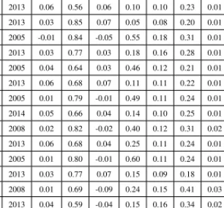
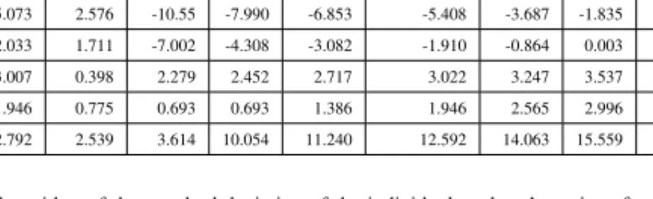
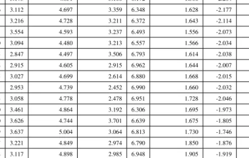
Table 2 shows the parameter estimates for the VAR(1) model. The table shows that all the industry–year sets of parameter estimates are stationary and will con-verge steadily to a long-run level (i.e. 0 < ρ <1and0 < β <1). Furthermore, as expected, the error terms from the two autoregressive processes are positively correlated (i.e.ψ >0)17_.

Table 2: Parameter Estimates

SIC Code Year γ ρ α β θ σ ψ No. Obs.

13 2007 0.10 0.45 0.08 0.42 0.12 0.24 0.02 222 13 2013 0.06 0.56 0.06 0.10 0.10 0.23 0.01 591 20 2013 0.03 0.85 0.07 0.05 0.08 0.20 0.01 273 28 2005 -0.01 0.84 -0.05 0.55 0.18 0.31 0.01 317 28 2013 0.03 0.77 0.03 0.18 0.16 0.28 0.01 636 35 2005 0.04 0.64 0.03 0.46 0.12 0.21 0.01 280 35 2013 0.06 0.68 0.07 0.11 0.11 0.22 0.01 607 36 2005 0.01 0.79 -0.01 0.49 0.11 0.24 0.01 376 36 2014 0.05 0.66 0.04 0.14 0.10 0.25 0.01 273 37 2008 0.02 0.82 -0.02 0.40 0.12 0.31 0.02 209 37 2013 0.06 0.68 0.04 0.25 0.11 0.24 0.01 300 38 2005 0.01 0.80 -0.01 0.60 0.11 0.24 0.01 311 38 2013 0.03 0.77 0.07 0.15 0.09 0.18 0.01 537 48 2008 0.01 0.69 -0.09 0.24 0.15 0.41 0.03 203 48 2013 0.04 0.59 -0.04 0.15 0.16 0.34 0.02 292 50 2013 0.09 0.45 0.08 0.04 0.09 0.17 0.01 255 73 2005 0.04 0.63 0.03 0.36 0.11 0.25 0.01 490 73 2013 0.07 0.60 0.06 0.31 0.11 0.23 0.01 995

Parameter estimates for the VAR1 model by 2-digit SIC code and fiscal year. For clarity, only the first and last fiscal year for each 2-digit SIC code are shown. In total there are 62 sets of parameter estimates distributed over 10 2-digit SIC code industries.

Tables 3 and 4 present the mean and median price deflated forecast errors (MPDE and MdPE), also known as the mean and median bias.

17_{For clarity, only the first and last fiscal year for each 2-digit SIC code are shown in Table 2. In total there are}

62 sets of parameter estimates distributed over 10 2-digit SIC code industries. The other 44 industry–year sets of parameter estimates that are untabulated are similar to the presented ones

Table 3: Forecast Bias—Mean Price Deflated Error

Model Period t+1 Period t+2 Period t+3 Period t+4 Period t+5

MPDE No. Obs. MPDE No. Obs. MPDE No. Obs. MPDE No. Obs. MPDE No. Obs.

FRAR1 −0.013 5961 −0.031 4406 −0.024 2489 −0.027 1889 −0.023 1500

Random Walk 0 5961 0 4406 0.007 2489 0.013 1889 0.015 1500

Analyst Forecast −0.022 5961 −0.044 4406 −0.046 2489 −0.063 1889 −0.077 1500

Forecast bias measured by the Mean Price Deflated Error (MPDE) over the five-year forecasting period for the proposed model in the paper (FRAR1), the Random Walk, and Analyst Forecasts. Periodt+kindicates thej-year ahead forecast. Firm–year observations are pooled, thus the fiscal year for forecasting periodt+kcould differ across firms (and also for a specific firm if forecasts are repeated for the same firm).

Table 3 shows that the FRAR1 model and the analyst forecasts are too optimistic (i.e., negative forecast bias) over the whole five-year forecasting period. The signs on the mean forecast bias for the RW model suggest that the RW model forecasts are unbiased in the first two years, whereas in the next three years they are too pessimistic (i.e., positive forecast bias). Furthermore, it shows that the RW model has the lowest (unsigned) mean forecast bias and that the analyst forecasts have the highest.

Table 4: Forecast Bias—Median Price Deflated Error

Model Period t+1 Period t+2 Period t+3 Period t+4 Period t+5

MdPDE No. Obs. MdPDE No. Obs. MdPDE No. Obs. MdPDE No. Obs. MdPDE No. Obs.

FRAR1 0.006 5961 0.006 4406 0.009 2489 0.011 1889 0.013 1500

Random Walk 0.004 5961 0.008 4406 0.012 2489 0.016 1889 0.018 1500

Analyst Forecast 0.003 5961 −0.003 4406 −0.004 2489 −0.01 1889 −0.017 1500

Forecast bias measured by the Median Price Deflated Error (MdPDE) over the five-year forecasting period for the proposed model in the paper (FRAR1), the Random Walk, and Analyst Forecasts. Periodt+kindicates thej-year ahead forecast. Firm–year observations are pooled, thus the fiscal year for forecasting periodt+kcould differ across firms (and also for a specific firm if forecasts are repeated for the same firm).

However, Table 4 shows that the FRAR1 model has the lowest (unsigned) me-dian forecast bias in forecasting in year five, whereas in years one to four, the analyst forecasts have the lowest. Furthermore, it shows that the RW model has

the highest (unsigned) median forecast bias in all years except year one, where the FRAR1 model have the highest. The signs of the median forecast bias show that the RW and FRAR1 model are too pessimistic, whereas the analyst forecasts are too optimistic (except for year one). Overall, the two tables do not clearly suggest which forecast has the lowest bias. On the other hand, Table 5 shows the percentage of forecasts where the forecast error is positive.

Table 5: Forecast Bias—Percentage of Positive Forecast Errors

Model Period t+1 Period t+2 Period t+3 Period t+4 Period t+5

PPPE No. Obs. PPPE No. Obs. PPPE No. Obs. PPPE No. Obs. PPPE No. Obs.

FRAR1 0.611 5961 0.569 4406 0.595 2489 0.608 1889 0.622 1500

Random Walk 0.618 5961 0.633 4406 0.681 2489 0.695 1889 0.722 1500

Analyst Forecast 0.558 5961 0.462 4406 0.442 2489 0.39 1889 0.322 1500

Forecast bias measured by the Percentage of Positive Forecast Errors (PPFE) over the five-year forecasting period for the proposed model in the paper (FRAR1), the Random Walk, and Analyst Forecasts. Periodt+kindicates thej-year ahead forecast. Firm–year observations are pooled, thus the fiscal year for forecasting periodt+kcould differ across firms (and also for a specific firm if forecasts are repeated for the same firm).

This shows that the FRAR1 model produces forecasts that are a little more often pessimistic than optimistic (around 60% of the time) for the whole forecasting period. However, Table 5 further shows that the RW model produces forecasts that more often are pessimistic compared to the FRAR1 model. As the forecast-ing horizon increases, the frequency of pessimistic forecasts relative to optimistic forecasts increases as well for the RW model. At the five-year forecasting hori-zon, the RW model produces pessimistic forecasts approximately 70% of the time. With respect to analyst forecasts, the pattern is almost the same as the RW model except that the analyst forecasts are too optimistic. This forecast optimism bias in analyst forecasts is in line with findings in earlier research.

Tables 6 and 7 present the mean and median absolute price deflated forecast errors (MAPDE and MdAPDE).

T able 6: F orecast Accurac y—Mean Absolute Price Deflated Error Model Period t+1 Period t+2 Period t+3 Period t+4 Period t+5 MAPDE No. Obs. MAPDE No. Obs. MAPDE No. Obs. MAPDE No. Obs. MAPDE No. Obs. FRAR1 0.07 5961 0.08 4406 0.078 2489 0.082 1889 0.078 1500 Random W alk 0.068 5961 0.078 4406 0.076 2489 0.077 1889 0.072 1500 Analyst F orecast 0.077 5961 0.086 4406 0.085 2489 0.095 1889 0.102 1500 F orecast accurac y measured by the Mean Absolute Price Deflated Error (MAPDE) ov er the fi ve-year forecasting period for the proposed model in the paper (FRAR1), the Random W alk, and Analyst F orecasts. Period t + k indicates the j -year ahead forecast. Firm–year observ ations are pooled, thus the fiscal year for forecasting period t + k could dif fer across firms (and also for a specific firm if forecasts are repeated for the same firm). T able 7: F orecast Accurac y—Median Absolute Price Deflated Error Model Period t+1 Period t+2 Period t+3 Period t+4 Period t+5 MdAPDE No. Obs. MdAPDE No. Obs. MdAPDE No. Obs. MdAPDE No. Obs. MdAPDE No. Obs. FRAR1 0.019 5961 0.025 4406 0.028 2489 0.032 1889 0.034 1500 Random W alk 0.014 5961 0.021 4406 0.024 2489 0.027 1889 0.027 1500 Analyst F orecast 0.018 5961 0.022 4406 0.022 2489 0.026 1889 0.03 1500 F orecast accurac y measured by the Median Absolute Price Deflated Error (MdAPDE) ov er the fi ve-year forecasting period for the proposed model in the paper (FRAR1), the Random W alk, and Analyst F orecasts. Period t + k indicates the j -year ahead forecast. Firm–year observ ations are pooled, thus the fiscal year for forecasting period t + k could dif fer across firms (and also for a specific firm if forecasts are repeated for the same firm).

Table 6 shows that the RW earnings forecasts are the most accurate in terms of MAPDE and that the analyst forecasts are the least accurate. In terms of MdAPDE, Table 7 shows that the FRAR1 model is the least accurate. This sug-gests that some of the analyst forecasts are much worse than the FRAR1 model, but analyst forecasts more often are more accurate than the FRAR1 model fore-casts.

5.1 Enhancing the forecast performance of FRAR1

The poor accuracy of the FRAR1 model compared to the RW model could be driven by the model specification. In the following, I propose two different rea-sons for the poor forecasting performance of the FRAR1 model relative to the RW model. Furthermore, I propose possible solutions for enhancing the forecasting performance of the FRAR1 model, in terms of accuracy, for future research. 5.1.1 Non-constant convergence rate

Fama and French (2000) find that “mean reversion is faster when profitability is below its mean and when it is further from its mean in either direction.” Likewise Hayn (1995) and Basu (1997) show that, on average, losses are less persistent than profits. Thus, estimating the time-series parameters separately for firms that are above and below the long-run level could enhance the accuracy of FRAR1. There are two ways to do this: either the estimation sample data could be split into two parts or the time-series parameters could be estimated from one sample where an interaction term between the lagged earnings and an indicator variable (which should take the value of one whenROE₀> ROELRand zero otherwise)

is included in the model. However, the latter method would lead to two different long-run levels, since the long-run level is equal to the constant divided by one

minus the autoregressive parameter.

Sloan (1996) find that there is a difference in persistence in the components of earnings, i.e., the cash flow component and the accruals component. Sloan (1996) find that cash flows are more persistent than accruals. Thus dividing earnings into cash flows and accruals might enhance the accuracy of forecasting from the FRAR1 model.

5.1.2 Segregation

The decomposition of financial ratios into a larger set of lower level ratios is widely used when analyzing financial statements, both in practice and in research. By segregating ROE (and/or the growth in book value of equity) into more com-ponents, forecasting accuracy can be enhanced. ROE can be decomposed (Nissim and Penman (2001)) into

ROE₌RN OA₊LEV₍RN OA₋N BC₎ (3) where RNOA is Return on Net Operating Assets, LEV is financial leverage, and NBC is net borrowing costs. Esplin et al. (2014) find that the forecasting accuracy of ROE can be enhanced by separately forecasting the components (the right hand side of Equation 3) ofROE. In addition, ROE could be decomposed even fur-ther by decomposing RNOA into profit margin (PM) and Asset Turnover (ATO). Fairfield and Yohn (2001) and Soliman (2008) find that the accuracy of forecast-ing the change in Return On Assets (ROA) can be enhanced by disaggregatforecast-ing the change in ROA into the change in PM and the change in ATO. Furthermore, Fairfield et al. (1996) decompose ROE additively in four steps: 1.) into nonre-curring and renonre-curring items, 2.) separating special items from renonre-curring items, 3.) separating operating earnings from recurring items without special items, 4.) a

full separation of line items (such as SGA expenses, depreciation, interest, tax). Fairfield et al. (1996) find that disaggregating ROE improves the forecasting ac-curacy and that the improvement increases with increasing disaggregation. Thus disaggregating ROE into lower level components could enhance the accuracy of forecasting from the FRAR1 model.

6 Robustness check

6.1 Industry definition

The definition of each industry probably influences the forecasting performance, since the “optimal” industry definition is the one that maximizes the homogeneity across firms of the time-series parameters for the ROE and growth in book value of equity. Homogeneity could be increased by increasing the number of industry segments. On the other hand, this would reduce the number of observations used to estimate the time-series parameters. Thus, choosing the “optimal” industry classification is a trade-off between homogeneity and sample size. The optimal industry classification is purely an empirical question. Using 2-digit NAICS codes as well as 1- and 2-digit SIC codes yield similar results.

6.2 Sample period

Time-series parameters can be highly influenced by a financial crisis. Including observations from the period of the financial crisis may lead to biased autore-gressive parameters as well as positively biased volatility estimates. Using only observations before the financial crisis (2007) yields similar results.