Forecasting Time Series from Clusters.

ISSN 1440-771X ISBN 0 7326 1064 8

M O N A S H U N I V E R S I T Y

AUSTRALIA

Forecasting Time Series From Clusters

Elizabeth A. Maharaj and Brett A. Inder

Working Paper 9/99 June 1999

DEPARTMENT OF ECONOMETRICS

AND BUSINESS STATISTICS

Forecasting Time Series from Clusters

Elizabeth A. Maharaj and Brett A. Inder

Monash University

Australia

Abstract

Forecasting large numbers of time series is a costly and time-consuming exercise. Before

forecasting a large number of series that are logically connected in some way, we can first

cluster them into groups of similar series. In this paper we investigate forecasting the series in

each cluster. Similar series are first grouped together using a clustering procedure that is based

on a test of hypothesis. The series in each cluster are then pooled together and forecasts are

obtained. Simulated results show that this procedure for forecasting similar series performs

reasonably well.

Keywords: Autoregressive models, Clustering technique, Mean square forecast error, Pooled

series,

1.

Introduction

Forecasting large numbers of logically connected time series especially in the short term is a

common occurrence in many situations. Some examples are inventory control, stocks and

shares, course enrolments at universities. While there is a vast literature on forecasting

methodologies, very little research has been done on forecasting similar series.

Shah (1997) discusses model selection in univariate time series forecasting. He

mentions that given a number of univariate time series, the forecaster may select one best

This rule is based on the classification technique of discriminant analysis. Discriminant analysis

requires known groupings of time series before any further series can be classified. However in

many situations, known groupings of the time series under consideration are not available.

Similar time series may be grouped together by some conventional clustering technique

(see Everitt 1993). The problem with conventional clustering techniques is its subjective nature.

The analyst must decide upon the number of clusters by selecting the distance at which the

clusters are to be identified. Maharaj (1996, 1997) proposed a method of clustering stationary

time series based on the p-value of a test of hypotheses that there is no difference between the

generating processes of every two series under consideration. This method of clustering is far

less subjective than the conventional clustering techniques. This method can also be

successfully applied to nonstationary time series that can be easily transformed to stationary

series.

In this paper we investigate the forecasting of series in each of the clusters which are

selected using the above-mentioned clustering technique. Simulated results will show that

when the series in a cluster are pooled together and fitted with an AR(k) model, the individual

series in this cluster now fitted with the pooled model produce on average more accurate

forecasts then when they are fitted with their own models. We will show theoretically that if

the pooled and individual models are of the same order k, where k = 1 or 2, the mean square

forecast error for the pooled model is less than that for the individual model for one-step ahead

forecasts.

In Section 2 we briefly discuss the clustering technique mentioned above. In Section 3

we show the theoretical results. The results of the simulation study are given and discussed in

Section 4 and in Section 5 we consider an application to a set of economic time series.

2.

Clustering of Time Series

H0: There is no difference between the generating processes of two stationary series

HA: There is a difference between the generating processes of two stationary series

Truncated AR(∞) models of order k, are fitted to each series and the test statistic which is based on the difference between the AR(k) estimates is constructed. These estimates are

generalised least squares estimates. The order k can be selected by criteria such as the Akaike's

information criterion (AIC) or the Schwarz's Bayesian information criterion (BIC). A

seemingly unrelated regressions model is used to construct the test statistic which follows a

chi-square distribution (see Maharaj (1997)).

The clustering procedure as given in Maharaj (1997) has the following steps: First

perform the test of hypothesis for every pair of series determining the p-value associated with

the test. Use these p-values in an algorithm that incorporates the principles of hierarchical

clustering but will only group together those series whose associated p-values are greater than

some predetermined significance level (for example 0.05 or 0.01). Simulation studies have

shown that this clustering procedure performs reasonably well.

3.

Theory

For k = 1 and 2 we will show that when m series with equal variance are pooled together and

fitted with an AR(k) model, this model when fitted to each of the m series will produce a

smaller mean square forecast error (MSFE) for the one-step ahead forecast than when each of

the m series is fitted with its own AR(k) model. We assume that the m series are generated from

the same stationary process and hence form a cluster.

Lemma 1

Consider an AR(k) model

t k t k 2 t 1 t t y y y a y =φ_{1 −} +φ_{2 −} +K+φ ₋ +

fitted to the time series {yt, t=1,2,…,T}. at is a white noise process with mean 0 and variance

2

a

σ

. Since this is a lag dependent model and since the AR(k) process is stationary

Q u ut ′=

∑

+ = T k t t plim 1 k -T 1 where

[

t t t k

]

t = y− y− . . . y− ′ 1 2 u and                   = kk k k k k q . . . q q . . . . . . . . . . . . . . . . . . q . . . q q q . . . q q 2 1 2 22 21 1 12 11 Q

is a finite positive definite matrix (see Greene (1993)).

Theorem 1: Assume that m series with equal variance are generated from the same

stationary process and that each series is fitted with an AR(k) model, where k = 1 or 2. Pool the

m series together and assume that this pooled series is also fitted with an AR model of the same

order k. Fit each of the m series with the pooled model. Then for one-step ahead forecasts

MSFEP < MSFEI

where MSFEI and MSFEP are the mean square forecast errors when a series is fitted with its

own model and with the pooled model respectively.

Proof: (a) k = 1

Consider an AR(1) model fitted to the time series {yt, t=1,2,…,T}

t t

t y a

where at is a white noise process with mean 0 and variance

σ

_a2. The one step ahead forecast for yt is 1 1 − = t t ˆ y y ˆ φ . (3.2)

Hence the forecast error is

(

)

t t

t t

t y yˆ ˆ y a

e = − = φ1−φ1 ₋1+ .

The mean square forecast error is

( )

(

)

( )

2 2 2 1 2 2 I MSFE a t t t t ˆ y E y ˆ y E e E σ φ φ _+   ₋ = − = = − (3.3) Then

(

)

(

)

(

)

( )

_   _{− −} = − − − 2 2 1 2 I 1 MSFE 1 T σ_a E y_t T φˆ φ .

Taking the limit as T →∞

( )

(

)

(

)

(

)

(

)

(

)

(

)

(

)

( )

y limE

(

T

)

(

ˆ

)

. E lim ˆ T lim y lim E ˆ T y lim E ˆ T y E lim T lim t t t t a     _{− −} =     _{− −} =     _      _{− −} =     _      _{− −} = − − − − − 2 1 1 2 1 2 1 1 2 1 2 1 1 2 1 2 1 1 2 1 2 I 1 1 1 1 MSFE 1 -φ φ φ φ φ φ φ φ σ (3.4)

Now since {yt, t=1, 2, . . . T} is a stationary series

( )

1 2 1 c y E lim t− =

where c1 is a constant. Furthermore

( )

(

)

( )

(

)

(

) (

)

1 1 -1 -1 2 2 1 1 2 1 1 − ′ − =     _      ₋ =     _      ₋ X X a T plim ˆ T E plim ˆ T E lim σ φ φ φ φ (3.5) where

[

1 2 −1

]

= ′ y y . . . yT X . Hence

(

) (

)

∑

= − − − = ′ − T t t a a y T plim T plim 2 2 1 2 1 2 1 1 1 σ XX σ , and by Lemma 1 1 11 2 2 1 1 1 c q y T plim T t t = = −

∑

= − .

Thus Equation (3.4) becomes

( )

(

)

2 1 2 1 2 I MSFE 1 - a a a c c T lim −σ = σ =σ . (3.6)

We now pool together m stationary time series y1 , y2,. . ., ym, thatare generated for the same

process, where

[

yi1 yi2 . . . yiT

]

= ′ i y

for i = 1, 2, . . . m. Fit the pooled series with an AR(1) model. The model for the pooled series

is now of the form

b W Z = φip + (3.7) where

[

]

( ) ( )

[

2 3 1 2 2 1 1 1 1 2 1

]

3 2 2 23 22 1 13 12 + − + − + − − + + = = ′ m mT T m T m T T T T mT m m T T z . . z z . . z . . z z z . . z z y . . y y . . y . . y y y . . y y Z

[

]

( ) ( ) ( ) ( )

[

1 2 1 1 2 1 1 1 1 1

]

1 2 1 1 2 22 21 1 1 12 11 − + − − − + − − − − = = ′ T m T m T m T T T T T m m m T T z . . z z . . z . . z z z . . z z y . . y y . . y . . y y y . . y y W

[

]

( ) ( )

[

2 3 1 2 2 1 1 1 1 2 1

]

3 2 2 23 22 1 13 12 + − + − + − − + + = = ′ m mT T m T m T T T T mT m m T T b . . b b . . b . . b b b . . b b a . . a a . . a . . a a a . . a a b

Since the series which are pooled together this manner are expected to be logically connected,

we assume that the disturbances are correlated across series. That is

[ ]

a

_it

a

_{jt ij}

I

E

=

σ

i, j = 1, 2, . . . , m

where I is a (T-1) × (T-1) identity matrix. Hence the variance of bis

[ ]

b

b

′

=

V

=

Ó

⊗

I

E

where





































=

mm m m m m

.

.

.

.

.

.

.

.

.

.

.

.

.

.

.

.

.

.

.

.

.

.

.

.

.

.

.

σ

σ

σ

σ

σ

σ

σ

σ

σ

2 1 2 22 12 1 12 11

Ó

and where it is assumed that

2 22

11 σ ... σmm σa

σ = = = =

It is also assume that the observations of the m series are uncorrelated with each other across

time.

As opposed to ordinary least squaresestimation of φ1 in (3.1), φ1P is now estimated by generalised least squares. That is

[

W′V−1W

] [

−1W′V−1Z

]

= P ˆ 1 φ .

Premultiplying the model in (3.7) by V−12 gives

b V W V Z V−12 = −12 φ1P+ −12 or * P * * b W Z/ = φ₁ + The variance of b* is

I

b

b

a2 * *

E

=

σ









′

_. Therefore

[

* *

]

* * P ˆ _{W W} 1_{W Z} 1 −     ′ = φ .

Hence fitting the pooled AR(1) model to each of the m series gives

t t P

t y a

y =φ_{1 −1}+ .

The one step-ahead forecast for yt is

1 1 − = P t t ˆ y y ˆ φ .

Following through steps similar to those in equations (3.3) to (3.5)

(

)

(

)

(

)

( )

(

)

(

)

(

)

( )

( ) . z T m plim c T m plim c ˆ T m E plim c T m lim T m t * t a a

∑

− + = − − =       ′ − =     _      ₋ = − − 1 1 2 2 1 2 a 1 1 2 1 2 1P P 1 1 2 P 1 -1 1 1 MSFE 1 σ σ φ φ σ * * W W As a consequence of Lemma 1

( )

( ) . c q z T m plim T m t * t 11 1 1 1 2 2 1 1 -1 = =

∑

− + = − Thus

(

)

(

)

m c m c T lim a a a 2 1 2 1 2 P MSFE 1 −σ = σ =σ − . (3.8)

Taking the ratio of (3.6) to (3.8)

(

)

(

)

m lim a a = − − 2 P 2 I MSFE MSFE σ σ . (3.9) Thus MSFEP < MSFEI

for large samples, with the mean square forecast error ratio proportional to the number of series

that are pooled together.

b) k=2

Consider an AR(2) model fitted to the time series {yt, t=1,2,…,T}.

t t t

t y y a

y =φ_{1 −1}+φ_{2 −2}+

where at is a white noise process. The one step ahead forecast for yt is

2 2 1 1 − + − = t t t ˆy ˆ y y ˆ φ φ .

Hence the forecast error is

(

) (

t

)

t t

t t

t y yˆ ˆ y ˆ y a

e = − = φ₁−φ_{1 −1}+ φ₂−φ_{2 −2}+ .

The mean square forecast error

( )

(

)

(

)

(

)

(

)(

)

[

y y ˆ ˆ

]

. E ˆ y E ˆ y E y ˆ y E e E a t t t t t t t 2 2 2 1 1 2 1 2 2 2 2 2 2 1 1 2 1 2 2 2 MSFE σ φ φ φ φ φ φ φ φ + − − +     ₋ +     ₋ = − = = − − − − (3.9)

Then taking the limit as T →∞and as a consequence of Lemma 1

(

)

(

)

(

)

(

)

(

)

(

)

[

(

)

(

)(

)

]

(

)

(

)

(

)

1 12 2 1 22 2 2 1 11 2 1 2 2 1 1 2 2 2 2 2 1 1 1 2 I 2 2 2 2 2 2 2 2 MSFE 2 − − − _{+ − + −} − = − − − +     _{− −} +     _{− −} = − − S T plim d S T m pli d S T plim d ˆ ˆ T E plim d ˆ T E plim d ˆ T E plim d T lim a 12 a a 12 a σ σ σ φ φ φ φ φ φ φ φ σ (3.10) where d1= q11, d2 = q22 , d12 = q12 , 1 ij

S

− , i,j =1, 2 is the ijth element of the matrix

(

X′X

)

−1 and

      = ′ − − 1 2 1 2 3 2 T T y . . . y y y . . . y y X .

Since both d1 and d2 represent the asymptotic variance of the time series, d1 = d2.

∑ ∑

∑

∑

= − = − = − − = − −     − = T t T t T t t t t t T t t y y y y y S 3 3 2 3 2 1 2 2 2 1 3 2 2 1 11

∑ ∑

∑

∑

= − = − = − − = − −     − = T t T t T t t t t t T t t y y y y y S 3 3 2 3 2 1 2 2 2 1 3 2 1 1 22

∑ ∑

∑

∑

= − = − = − − = − − − −     = T t T t t t T t t t T t t t y y y y y y S 3 3 2 2 2 1 2 3 2 1 3 2 1 1 12 . Hence

(

)

(

)

. d d d y y T plim y y T plim y T plim y T plim y T plim S T plim _T t T t T t t t T t t t t t T t t 2 12 2 1 1 3 3 3 2 1 3 2 1 2 2 2 1 3 2 2 1 11 2 1 2 1 2 1 2 1 2 1 2 − = − − − − − − = −

∑

∑

∑

∑

∑

= − = − = − − = − − = − − Similarly

(

2

)

12 2 1 1 1 22 d d d S plim − = −

(

2

)

12 12 d d d S plim − − = − 2 1 1 12 .

Hence Equation (3.10) becomes

(

)

(

)

2 2 12 2 1 2 12 2 1 2 2 2 2 2 MSFE 2 a a a d d d d T lim σ σ σ =       − − = − − (3.11)

So now if m stationary time series y1, y2, . . . ,ym are generated for the same process and

are pooled together and fitted with an AR(2) model, it can be shown in a similar manner to that

(

)

(

)

m lim a a 2 2 P 2 MSFE 2 -T −σ = σ . Hence

(

)

(

)

m lim a a = − − 2 P 2 I MSFE MSFE σ σ . So again MSFEP < MSFEI.

for large samples, with the mean square forecast error ratio proportional to the number of series

that are pooled together.

The results of Theorem 1 can also be extended to series fitted with AR(k) models

giving

(

)

(

2

)

2 I MSFE a k a k T lim − −σ = σ

(

)

(

)

m k k T lim a a 2 2 P MSFE −σ = σ −

It is clear that as the number of series in a cluster increases the greater the effect of the

pooled model on the mean square forecast error. It should however it noted that for all values of

k, as T increases, the difference between MSFEP and MSFEI decreases.

4.

Simulation Study

4.1. Design

The simulation study was carried out in two stages :

(a) Two groups of two series each:Two series were generated from each of an AR(1)

process with φ=0.5 and a MA(1) process with θ = 0.9. Each of the four series were fitted with AR(k) models. The two series generated from the AR(1) model were pooled together and the

pooled series was fitted with an AR(k) model. Likewise the two series generated from the

MA(1) model were pooled together and the pooled series was fitted with an AR(k) model.

(b) Two groups of eight series each: Eight series were generated from each of an AR(1)

process with φ=0.5 and a MA(1) process with θ = 0.9. Each of the sixteen series were fitted with AR(k) models. The eight series generated from the AR(1) model were pooled together and

the pooled series was fitted with an AR(k) model. Likewise the eight series generated from the

MA(1) model were pooled together and the pooled series was fitted with an AR(k) model.

For stage (a) series lengths of T=50 and 200 were taken when it was assumed that the

correlation between the disturbances of each pair of processes from which the series were

generated was in turn 0 and 0.5. For stage (b) series lengths of T=50 and 200 were taken when

it was assumed that the correlation between the disturbances of each pair of processes from

which the series were generated was 0. When it was assumed that the correlation between the

disturbances of each pair of processes from which the series were generated was 0.5, series

lengths of only T 1=50 was taken. One, two and five-step-ahead forecasts were obtained for

each series fitted with their own autoregressive models as well as for each series fitted with the

relevant pooled autoregressive model. Each time the models were fitted to T-h (h=1,2,5)

observations for the individual series and to m(T-h) observations for pooled series, (m=2,8).

The mean square forecast error for both the pooled and individual models were determined for

the h out of sample values. The Akaike's (AIC) and the Schwarz's Bayesian (BIC) criteria were

used to select the order of the AR model. One thousand simulations were carried out for each

series length, selection criterion and h (1,2 5) step ahead forecast, for each of stages (a) and (b).

Average mean square forecast error were determined for the series in each group, when the

series were fitted with their own AR models as well as with the relevant pooled AR model.

95% prediction intervals were also obtained for the forecasts and the average number of times

this interval contained the true value was observed for each group.

1

For series length T=200, the simulations were unmanageable because of restrictions on the work space requirements of the computer program.

4.2 Discussion

For both uncorrelated and correlated series, it can be seen from Tables 1, 2, 3 and 4, for stage

(a), and from Tables 5, 6 and 7 for stage (b) that the group average mean square forecast error

is always smaller when the series were fitted with the pooled model than when the series were

fitted with their own models. In most cases the percentage decrease in average mean square

forecast error is greatest for the one-step ahead forecasts. The percentage decrease in average

mean square forecast error in all cases is greater when the series in the group were generated

from the MA(1) process with θ = 0.9 than from the AR(1) process with φ = 0.5.

< INSERT TABLES 1, 2, 3, 4, 5, 6, 7 HERE>

For both stages (a) and (b), the percentage decrease in the group average mean square

forecast error between the individual and pooled models is greater for series length 50 than for

series length 200. Comparing the results for the uncorrelated and correlated series in Table 1

with 5, 2 with 6 and 3 with 7, it can be seen that the percentage decrease in the group average

mean square forecast error between the individual and pooled models are fairly similar.

Comparing the results of Tables 1, 2 and 3 with that of Tables 5, 6 and 7 respectively, it

is clear that in almost all cases the percentage decrease in the group average mean square

forecast error is greater for groups with eight series each, than for groups with two series each.

These observations are consistent with the theoretical results in Section 3 even though the

autoregressive models that were fitted to the individual series and to the pooled series within a

group were not necessarily of the same order.

It can also be seen that in almost all cases lower group average mean square forecast

errors were obtained for the pooled model than for the corresponding individual model when

From Tables 8, 9, 10 and 11 for stage (a) and from Tables 12, 13 and 14 for stage (b), it

can be seen that in almost all cases, the average number of times the 95% prediction interval in

each group contains the true value of the forecast is almost always greater when the pooled

model was fitted to the series. However, it is mostly for the one-step-ahead forecasts, for the

pooled model cases, that the true value of the forecast lies in the prediction interval close to

95% of the time.

< INSERT TABLES 8,9,10,11,12,13,14 HERE>

5.

Application

Consider the time series of the number of dwelling units financed by all lenders (banks and

other institutions) in the states and territories of Australia from January 1978 to March 1998.

Clearly these series are related since they are all influenced by the same economic factors. The

natural logarithm transformation of each series is shown in Figure 1 from where it is clear the

all these series2 are non-stationary. Some series appear to have fairly similar patterns.

However one cannot clearly distinguish how similar or how different these patterns are. First

differencing of each of these series appeared to render them stationary. The algorithm of

clustering procedure of Maharaj (1997) was then applied to these differenced series.

<INSERT FIGURE 1 HERE>

When the level of significance was set at 5% the algorithm produced the following

clusters : (NSW, NT), (OLD, SA, WA), (VIC, ACT) and (TAS). Graphs of the undifferenced

series for each of the three clusters are given in Figures 2 - 4, from where it is quite clear that

the patterns of the series from each cluster are similar. However it can be seen from these

figures that the series from a particular cluster are not necessarily on the same level. The reason

for this is that while the test of hypothesis on which the clustering algorithm is based

differentiates between stochastic nature of series it does not differentiate between their

corresponding deterministic nature. Hence it is possible for series at different levels but similar

2

patterns to cluster together. However this in no way affects any further analysis of the series in

<INSERT FIGURES 2- 4 HERE>

each cluster. For example, forecasts of the original series in a particular cluster will be obtained

by reversing the operation of differencing and any other transformation on the stationary series.

The standardised first difference of the logarithm of each the series excluding the March

1998 value, in each of the clusters (NSW, NT), (QLD, SA, WA), (VIC, ACT), were pooled

together and fitted with the relevant AR(k) model. The residual correlations between the series

in each cluster is given in Table 15, from where it is clear that the series are related.

<INSERT TABLE 15 HERE>

The forecasts from the pooled and individual models, percentage decrease in the mean square

forecast error between and individual and pooled models of each of the series as well as the

percentage decrease in group average mean square forecast error between the pooled and

individual models for the one-step-ahead forecasts, (that is for March 1998) are given in Table

16. These results were obtained when the BIC was used to select k. Similar results were also

obtained when the AIC was used to select k. With the exception of series TAS (which forms its

own cluster), NT and ACT, all the other series have smaller mean square forecast errors for the

pooled model than for the individual model. On average the mean square forecast error of each

group is smaller for the pooled than for the individual models.

<INSERT TABLE 16 HERE>

Forecasts were then obtained for the original series in each cluster. The results which are

given in Table 17 show that fitting the pooled model to the standardised first difference of the

logarithm of the series, produced on average more accurate one-step ahead forecasts than when

the series are fitted with their own models.

<INSERT TABLE 17 HERE>

Two and five-step ahead forecasts were also obtained, but the results showed that in

these cases there was no advantage in pooling the series in the clusters.

6.

Concluding Remarks

From both the theoretical and simulated results, it is clear that fitting a pooled model to all

series in a particular cluster produces more accurate forecasts than when the series are fitted

with their own models. The outcome of the application shows that the results are generally

consistent with the theory.

So while there isn't overwhelming evidence to support the use of a pooled model over

that of an individual model for forecasting, it would appear that it is worthwhile giving some

consideration to forecasting each series in a cluster from the pooled model.

Acknowledgments

This research was supported in part by a grant from the Monash University Research

Fund and in part by a grant from the Faculty of Business and Economics of Monash University.

References

Green, W.H. (1993), Econometric Analysis, Second Edition, Macmillan Publishing Company,

New York, 1993.

Everitt, B.S. (1993), Cluster Analysis, Halsted Press, New York.

Maharaj, E.A. (1996), A Significance Test for Classifying ARMA Models, Journal of

Statistical Computation and Simulation, 54, 305-331.

Maharaj, E.A. (1997), Pattern Recognition Techniques for Time Series, unpublished Ph.D.

thesis, Monash University.

Shah, C (1997), Model Selection in Univariate Time Series Forecasting using Discriminant

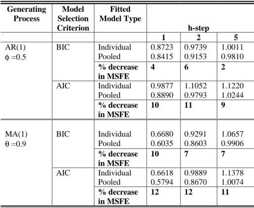
Table 1: Average mean square forecast error: 2 groups of 2 series, T=50, Corr=0 Generating Process Model Selection Criterion Fitted Model Type h-step 1 2 5

AR(1) BIC Individual 0.8723 0.9739 1.0011

φ =0.5 Pooled 0.8415 0.9153 0.9810 % decrease in MSFE 4 6 2 AIC Individual 0.9877 1.1052 1.1220 Pooled 0.8890 0.9793 1.0244 % decrease in MSFE 10 11 9

MA(1) BIC Individual 0.6680 0.9291 1.0657

θ =0.9 Pooled 0.6035 0.8603 0.9906 % decrease in MSFE 10 7 7 AIC Individual 0.6618 0.9889 1.1378 Pooled 0.5794 0.8670 1.0074 % decrease in MSFE 12 12 11

Table 8: Average number of times the 95% prediction interval of the forecast contains the true value per group: 2 groups of 2 series, T=50, Corr=0

Generating Process Model Selection Criterion Fitted Model Type h-step 1 2 5

AR(1) φ =0.5 BIC Individual 922 967 944 970 949 955 952 951 Pooled 932 977 958 976 955 960 952 952 AIC Individual 932 977 958 976 955 960 952 952 Pooled 933 973 957 981 959 965 962 963 MA(1) θ =0.9 BIC Individual 921 986 958 993 971 960 969 973 Pooled 946 996 969 997 979 971 974 981 AIC Individual 915 987 958 995 974 966 968 974 Pooled 954 997 975 996 984 978 981 983

Table 2: Average Mean Square Forecast Error: 2 Groups of 2 Series, T=200, Corr=0 Generating Process Model Selection Criterion Fitted Model Type h-step 1 2 5

AR(1) BIC Individual 0.7687 0.8541 0.9201

φ =0.5 Pooled 0.7679 0.8523 0.9169 % decrease in MSFE 0.1 0.2 0.3 AIC Individual 0.7968 0.8759 0.9486 Pooled 0.7851 0.8698 0.9383 % decrease in MSFE 2 0.7 1

MA(1) BIC Individual 0.5752 0.8328 0.9509

θ =0.9 Pooled 0.5590 0.8231 0.9355 % decrease in MSFE 3 1 2 AIC Individual 0.5621 0.8338 0.9505 Pooled 0.5501 0.8123 0.9336 % decrease in MSFE 2 3 2

Table 9: Average number of times the 95% prediction interval of the forecast contains the true value per group: 2 groups of 2 series, T=200, Corr=0

Generating Process Model Selection Criterion Fitted Model Type h-step 1 2 5

AR(1) φ =0.5 BIC Individual 943 985 963 983 972 974 970 969 Pooled 944 986 964 985 971 974 968 969 AIC Individual 939 983 963 986 974 972 971 974 Pooled 944 985 966 987 977 974 975 975 MA(1) θ =0.9 BIC Individual 949 998 983 998 981 983 984 989 Pooled 951 999 987 999 984 985 987 989 AIC Individual 944 999 984 999 982 987 988 991 Pooled 952 999 989 999 986 987 988 990

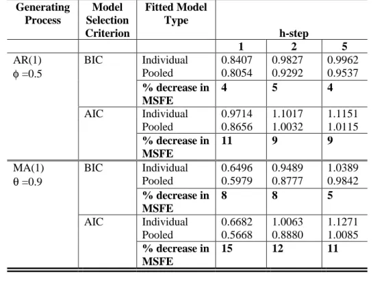
Table 3: Average mean square forecast error: 2 groups of 2 series, T=50, Corr=0.5 Generating Process Model Selection Criterion Fitted Model Type h-step 1 2 5

AR(1) BIC Individual 0.8407 0.9827 0.9962

φ =0.5 Pooled 0.8054 0.9292 0.9537 % decrease in MSFE 4 5 4 AIC Individual 0.9714 1.1017 1.1151 Pooled 0.8656 1.0032 1.0115 % decrease in MSFE 11 9 9

MA(1) BIC Individual 0.6496 0.9489 1.0389

θ =0.9 Pooled 0.5979 0.8777 0.9842 % decrease in MSFE 8 8 5 AIC Individual 0.6682 1.0063 1.1271 Pooled 0.5668 0.8880 1.0085 % decrease in MSFE 15 12 11

Table 10: Average number of times the 95% prediction interval of the forecast contains the true value per group: 2 groups of 2 series, T=50, Corr=0.5

Generating Process Model Selection Criterion Fitted Model Type h-step 1 2 5

AR(1) φ =0.5 BIC Individual 933 969 940 975 956 954 953 950 Pooled 944 979 950 980 961 966 957 951 AIC Individual 904 956 923 986 952 956 953 943 Pooled 942 975 947 980 963 970 968 959 MA(1) θ =0.9 BIC Individual 918 987 951 993 975 972 974 974 Pooled 949 995 974 994 982 979 984 984 AIC Individual 915 990 953 993 974 975 972 975 Pooled 956 996 976 996 984 987 986 985

Table 4: Average Mean Square Forecast Error: 2 Groups of 2 Series, T=200, Corr=0.5 Generating Process Model Selection Criterion Fitted Model Type h-step 1 2 5

AR(1) BIC Individual 0.8036 0.8443 0.9764

φ =0.5 Pooled 0.8034 0.8414 0.9741 % decrease in MSFE 0 0 0 AIC Individual 0.8294 0.8682 1.0009 Pooled 0.8202 0.8550 0.9897 % decrease in MSFE 1 2 1

MA(1) BIC Individual 0.6219 0.6219 0.9540

θ =0.9 Pooled 0.5963 0.5693 0.9407 % decrease in MSFE 4 4 1 AIC Individual 0.5953 0.8429 0.9627 Pooled 0.5765 0.8166 0.9435 % decrease in MSFE 3 3 2

Table 11: Average number of times the 95% prediction interval of the forecast contains the true value per group: 2 groups of 2 series, T=200, Corr=0.5

Generating Process Model Selection Criterion Fitted Model Type h-step 1 2 5

AR(1) φ =0.5 BIC Individual 945 977 972 984 972 958 954 959 Pooled 945 980 974 983 974 960 957 962 AIC Individual 936 977 961 986 975 965 959 966 Pooled 942 981 971 987 977 967 964 969 MA(1) θ =0.9 BIC Individual 940 999 980 999 988 985 987 987

Pooled 945 1000 985 999 990 989 988 989 AIC Individual 942 1000 1000 999 988 985 987 990 Pooled 949 981 986 999 993 989 991 992

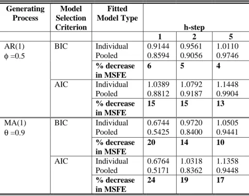
Table 5: Average mean square forecast error: 2 groups of 8 series, T=50, Corr =0 Generating Process Model Selection Criterion Fitted Model Type h-step 1 2 5

AR(1) BIC Individual 0.9144 0.9561 1.0110

φ =0.5 Pooled 0.8722 0.9130 0.9808 % decrease in MSFE 5 5 3 AIC Individual 1.0389 1.0792 1.1448 Pooled 0.9016 0.9302 1.0004 % decrease in MSFE 13 14 13

MA(1) BIC Individual 0.6744 0.9721 1.0505

θ =0.9 Pooled 0.5617 0.8500 0.9515 % decrease in MSFE 17 13 9 AIC Individual 0.6764 1.0318 1.1355 Pooled 0.5498 0.8493 0.9536 % decrease in MSFE 19 18 16

Table 12: Average number of times the 95% prediction interval of the forecast contains the true value per group: 2 groups of 8 series, T=50, Corr=0

Generating Process Model Selection Criterion Fitted Model Type h-step 1 2 5

AR(1) φ =0.5 BIC Individual 915 964 948 970 953 953 952 952 Pooled 931 974 961 978 961 961 960 956 AIC Individual 894 949 932 968 950 951 952 951 Pooled 946 981 970 986 976 976 972 970 MA(1) θ =0.9 BIC Individual 922 988 955 992 971 972 972 975 Pooled 963 997 980 997 986 985 984 984 AIC Individual 918 988 956 993 975 973 972 974 Pooled 970 998 985 998 989 989 987 990

Table 6: Average Mean Square Forecast Error: 2 Groups of 8 Series, T=200, Corr=0 Generating Process Model Selection Criterion Fitted Model Type h-step 1 2 5

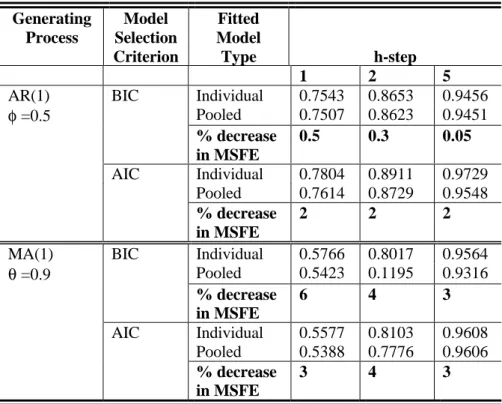
AR(1) BIC Individual 0.7543 0.8653 0.9456

φ =0.5 Pooled 0.7507 0.8623 0.9451 % decrease in MSFE 0.5 0.3 0.05 AIC Individual 0.7804 0.8911 0.9729 Pooled 0.7614 0.8729 0.9548 % decrease in MSFE 2 2 2

MA(1) BIC Individual 0.5766 0.8017 0.9564

θ =0.9 Pooled 0.5423 0.1195 0.9316 % decrease in MSFE 6 4 3 AIC Individual 0.5577 0.8103 0.9608 Pooled 0.5388 0.7776 0.9606 % decrease in MSFE 3 4 3

Table 13: Average number of times the 95% prediction interval of the forecast contains the true value per group: 2 groups of 8 series, T=200, Corr=0

Generating Process Model Selection Criterion Fitted Model Type h-step 1 2 5

AR(1) φ =0.5 BIC Individual 947 981 966 982 967 970 966 967 Pooled 948 980 967 982 970 970 967 970 AIC Individual 942 978 963 982 970 972 970 971 Pooled 947 981 969 988 978 977 975 978 MA(1) θ =0.9 BIC Individual 950 998 987 998 985 985 989 988 Pooled 961 999 992 999 988 989 991 991 AIC Individual 948 998 987 998 985 986 989 989 Pooled 962 999 992 999 989 989 991 992

Table 7: Average mean square forecast error: 2 groups of 8 series, T=50, Corr =0.5 Generating Process Model Selection Criterion Fitted Model Type h-step 1 2 5

AR(1) BIC Individual 0.9144 0.9561 1.0110

φ =0.5 Pooled 0.8594 0.9056 0.9746 % decrease in MSFE 6 5 4 AIC Individual 1.0389 1.0792 1.1448 Pooled 0.8812 0.9187 0.9904 % decrease in MSFE 15 15 13

MA(1) BIC Individual 0.6744 0.9720 1.0505

θ =0.9 Pooled 0.5425 0.8400 0.9441 % decrease in MSFE 20 14 10 AIC Individual 0.6764 1.0318 1.1358 Pooled 0.5171 0.8362 0.9448 % decrease in MSFE 24 19 17

Table 14: Average number of times the 95% prediction interval of the forecast contains the true value per group: 2 groups of 8 series, T=50, Corr=0.5

Generating Process Model Selection Criterion Fitted Model Type h-step 1 2 5

AR(1) φ =0.5 BIC Individual 915 964 947 969 952 952 952 951 Pooled 934 976 965 979 964 962 960 957 AIC Individual 893 984 931 967 950 950 952 951 Pooled 948 983 975 988 979 976 974 974 MA(1) θ =0.9 BIC Individual 922 987 954 991 971 971 971 974 Pooled 964 998 986 998 990 988 989 990 AIC Individual 918 988 954 993 974 972 972 973 Pooled 976 999 991 999 993 991 992 993

Table 15: Residual correlations between series in each cluster Cluster Correlation 1 NSW, NT 0.4854 2 QLD, WA 0.7209 QLD, SA 0.7333 WA, SA 0.6964 3 VIC, ACT 0.5844

Table 16: Forecast statistics for March 1998 of the standardised first difference of the logarithm of the series

Actual value of the standardised first difference of the log of original series Forecast from individual model Forecast from pooled model % Decrease in MSFE between individual and pooled models NSW -0.4205 0.3923 0.1699 47 VIC -0.1038 0.2789 0.1977 38 QLD -0.1845 0.1721 -0.0149 77 SA -0.4554 0.4485 -0.0315 78 WA -0.1429 0.2838 -0.0804 98 TAS 0.0372 0.2483 0.2483 0 NT -0.0967 0.1782 0.1825 - 3 ACT 0.5477 0.4251 0.4190 -10 Group % Decrease in the group average MSFE between the individual and pooled models (NSW, NT) 42 (QLD,SA,WA) 81 (VIC,ACT) 33 Table 17 Foreecast statistics for March 1998 of the original series Actual value of original series Forecast from individual model Forecast from pooled model % Decrease in MSFE between individual and pooled models NSW 14048 12322 12772 45 VIC 10147 9584 9701 37 QLD 6568 6214 6397 77 SA 3321 2925 3129 77 WA 5491 5154 5440 98 TAS 393 819 819 0 NT 682 366 366 0 ACT 848 694 695 1

Group % Decrease in the group average MSFE between the individual and pooled models

(NSW, NT) 44

(QLD,WA,SA) 83

(VIC, ACT) 35

Figure 1 Number of dwelling units financed from January 1978 to March 1998 for all states and territories

Figure 2 Number of dwelling units financed from January1978 to March 1998 for New South Wales and the Northern Territory

4 5 6 7 8 9 10 11

JAN.1978 JUL.1980JAN.1983 JUL.1985JAN.1988 JUL.1990JAN.1993 JUL.1995JAN.1998

month

natural log of number of dwelling units

financed WA SA TAS ACT NT VIC QLD NSW 4 5 6 7 8 9 10

JAN.1978 JUL.1980 JAN.1983 JUL.1985 JAN.1988 JUL.1990 JAN.1993 JUL.1995 JAN.1998 month

natural log of the number of

dwelling units financed

NSW NT

Figure 3 Number of dwelling units financed from January 1978 to March 1998 for Queensland, South Australia and Western Australia

Figure 4 Number of dwelling units financed from January 1978 to March 1998 for Victoria, Australian Capital Territory and Tasmania

7.0 7.5 8.0 8.5 9.0 9.5

JAN.1978 JUL.1980 JAN.1983 JUL.1985 JAN.1988 JUL.1990 JAN.1993 JUL.1995 JAN.1998 month

natural log of the number of

dwelling units financed

QLD SA WA 5 6 7 8 9 10

JAN.1978 JUL.1980 JAN.1983 JUL.1985 JAN.1988 JUL.1990 JAN.1993 JUL.1995 JAN.1998

month

natural log of the number of

dwelling units financed

VIC ACT