No. 14-
7
Student Loan Debt and Economic Outcomes
Daniel Cooper and J. Christina Wang
Abstract
This policy brief advances the growing literature on how student loan debt affects individuals’ other economic decisions. Specifically, it examines the impact of student loan liabilities on individuals’ homeownership status and wealth accumulation. The analysis employs a rich set of financial and demographic control variables that are not available in many of the existing studies that use credit bureau data. Overall, student debt lowers the likelihood of homeownership for a group of students who attended college during the 1990s. There is also a fairly strong negative correlation between student loan debt and wealth (excluding student loan debt) for a group of households with at least some college experience.
JEL codes: E20, E21
Daniel Cooper is a senior economist in the research department at the Federal Reserve Bank of Boston. J. Christina Wang is a senior economist and policy advisor the research department at the Federal Reserve Bank of Boston. Their email addresses are daniel,cooper@bos.frb.org and christina.wang@bos.frb.org, respectively.
This brief, which may be revised, is available on the web site of the Federal Reserve Bank of Boston at http://www.bostonfed.org/economic/ppdp/index.htm.
The views expressed herein are those of the authors and do not indicate concurrence by other members of the research staff or principals of the Board of Governors, the Federal Reserve Bank of Boston, or the Federal Reserve System.
We would especially like to thank Viacheslav (Slavik) Sheremirov for his extremely detailed and thoughtful comments and suggestions. We would also like to thank Ye Ji Kee for excellent research assistance.
1
Background
The swift rise in the stock of student loan debt in recent years—even during the Great Recession when other types of consumer debt contracted—has received much attention among researchers, politicians, and the media. Indeed, student loan debt has now surpassed credit card debt to become the second largest amount of household debt outstanding after mortgage debt (see Figure 1). Unlike credit card debt and other household liabilities, however, student debt cannot be discharged in bankruptcy. It therefore represents a long-term financial burden for many individuals and/or households that must be repaid. A key question is how student loan debt may impact individuals’ economic outcomes. For example, it could hinder an individual’s or household’s ability to obtain a mortgage and purchase a home.
To date, there has been much analysis of the evolution of student loan debt and its place on the liabilities side of household balance sheets (see, for example, Brown et al.,2012,
2014), but much less work examining the impact of student loan debt on homeownership and other economic outcomes. The existing research is limited in part by the availability of data: most data come from credit bureau records, such as the Federal Reserve Bank of New York’s Consumer Credit Panel (NY CCP), which offer detailed information on individuals’ liabilities but very limited demographic information and no data on financial assets. For instance, the NY CCP contains no education data and so it is not possible to distinguish individuals who went to college but did not accrue any debt from individuals who have no student debt because they never attended college. Individuals who attended college without college loans or individuals who repaid student debt soon after finishing school are likely to differ substantially from individuals who never attended college. This potential disparity in education levels among individuals without any student loan debt makes it difficult to interpret results that compare economic outcomes for these individuals using credit bureau data.
question of ultimate interest: are students making optimal decisions regarding how much education to pursue and how much to borrow to fund this learning? For instance, some observers have voiced the concern that some students may be borrowing too much for col-lege and instead would have benefited more, on net, from less costly, alternative training. Following the standard formulation (see, for example, Ionescu, 2012), optimal behavior is defined in terms of maximizing the present value of one’s life-time utility (or earnings) net of the borrowing. As the extensive literature on the return to education attests (see, for example, Carneiro, Heckman, and Vytlacil, 2010, and the studies referenced therein), opti-mal educational investment is an extremely difficult question to address because one needs to estimate an individual’s counterfactual life-time wealth had he/she made an alternative choice of education and the related borrowing. Overcoming this identification problem us-ing, for instance, an instrumental variables approach is difficult because there are few valid yet reasonably strong instruments. Examining the issue of optimal educational investment with borrowing is challenging overall and not feasible using our data, but we can analyze related issues that can be answered without a fully structural analysis, such as the relation-ship between student loan debt and household asset accumulation. We intend to explore the important question of optimal borrowing to finance higher education in future studies.
This policy brief expands upon and augments the relatively limited existing literature on student debt and economic outcomes using two alternative datasets—the Panel Study of Income Dynamics (PSID) and the 1988 National Educational Longitudinal Survey (NELS88). First, we utilize a recently added PSID variable on student debt liabilities in 2011 and 2013 to examine households’ student debt holdings against a much broader set of demographic characteristics and financial information than is available in the NY CCP. Second, we use detailed information in the NELS88 on individuals’ schooling history, ability, parents, debt, and homeownership status to inform the debate on whether student loan debt has a negative impact on homeownership. Given the dramatic rise in outstanding student debt liabilities, a
strong negative relationship between student loan debt and homeownership can have adverse implications for the U.S. homeownership rate and residential investment going forward.
We find that conditional on having at least some college experience, households with student debt have lower overall homeownership rates than similar households without stu-dent loan liabilities. This is particularly true among college graduates 30-to-40 years old. In addition, the distribution of total wealth excluding student debt liabilities is lower for home-owners with student debt than for homehome-owners without student loan debt (again conditional on at least some college attendance). This wealth disparity remains even after controlling for a wide range of demographic and other factors. In contrast, the distribution of wealth for renters, with and without student loan debt, is quite similar. We also show that student loan debt lowers the likelihood of homeownership for a representative group of individuals who were college age in the early 1990s. This result holds conditional on an individual’s ability, family characteristics, and a variety of demographic factors.
The remainder of this brief proceeds as follows. Section 2 reviews the recent and related literature on student loan debt, and Section 3 provides an overview of the two datasets used for the analysis. Section 4 presents our results, and Section 5 concludes.
2
Existing Literature
There are two threads in the existing literature on student debt. The first quantifies and evaluates the amount of student debt outstanding along with the performance (delinquency) of such debt, while the other examines the relationship between student debt and economic outcomes. Trends in student debt holdings and delinquency are discussed in Brown et al.
(2014), with earlier related work inBrown et al. (2012). Among other things, Brown et al.
(2014) note that, according to the NY CCP data, student loan debt recently surpassed credit card debt and became the largest amount of household debt outstanding other than
mortgage debt. In addition, student loan debt continued to rise during the financial crisis and the Great Recession, while all other types of household debt declined. The authors further show that the delinquency rate among student debt holders currently repaying their loans is quite high.1 The data also suggest that student loan holders have had a more difficult time
obtaining credit in the aftermath of the Great Recession than individuals without student debt.
Other research, including Brown and Caldwell (2013), examines the relationship between student debt and individuals’ other economic outcomes. Using NY CCP mortgage debt data to infer homeownership for individuals in the survey, the authors show that 30-year-olds with a history of student loans have higher homeownership rates between 2003 and 2009 than 30-year-olds without student debt. This relationship switched in the aftermath of the Great Recession as 30-year-olds without student loan debt had slightly higher homeownership rates than 30-year-olds with student loan debt.2 There was also a steeper decline in auto loan debt
outstanding for individuals with student loan debt in the aftermath of the Great Recession— suggesting fewer new or late model used car purchases among this group. The authors propose two reasons for this shift in economic outcomes: lower future income expectations following the recession for individuals with student loan debt, or more limited access to additional credit based on these individuals’ existing debt, or both.
Houle and Berger(2014) examine the relationship between student loan debt and home-ownership more directly using data from the National Longitudinal Study of Youth 1997 (NLSY97). One of the drawbacks of the NY CCP data is that one cannot observe homeown-ership directly. More importantly, the NY CCP data cannot distinguish between individuals who have zero debt because they never attended college and those individuals who attended
1
A large share, 44 percent, of individuals with student loan debt in the NY CCP are neither delinquent nor paying down their student loans. This represents people likely still in school, in deferral, or in forbearance on their payments.
2
Homeownership in the NY CCP is not directly observed, but rather is inferred based on mortgage debt data.
college but have zero debt—two groups of individuals who likely have substantially differ-ent resources and hence differdiffer-ent consumption (including housing) and investmdiffer-ent behavior.
Houle and Berger (2014) evaluate the conditional impact of student loan debt on homeown-ership while controlling for an individual’s education and other individual-level financial and demographic factors. They find a statistically significant, but not economically meaningful, relationship between student loan debt and homeownership, and conclude that student loan debt does not substantially impact the housing market.
We contribute to this existing literature by examining how student debt impacts home-ownership prior to the housing boom and the ensuing financial crisis. We pay particular attention to ensure “apples-to-apples” comparisons between individuals with and without student debt. In particular, we restrict our analysis to individuals who have attended college for at least some years. We also examine whether student loan debt impacts the financial well-being (that is, asset holdings, liabilities, and net worth) of individuals 40 years old and younger outside of their student loan liabilities, and how this well-being varies with housing tenure (that is, owner versus renter status).
3
Data
The PSID is a representative survey of U.S. households that began in 1968 and follows the original households and their offspring over time. Sixty percent of the initial 4,800 households surveyed belonged to a cross-national sample from the 48 contiguous states, while the other portion was a national sample of low-income families from the Survey of Economic Opportunity. The PSID was conducted annually through 1997 and since then has occurred biennially. The 2011 wave of the PSID includes close to 9,000 households.
The PSID also contains wealth supplements for 1984, 1989, 1994, and 1999 onward, which include detailed information on households’ financial positions including both their assets and
their liabilities.3 In 2011, the PSID started disaggregating a household’s overall nonhousing
liabilities, which had previously been reported in a single sum, into various components, one of which is their outstanding student loan balances. Preliminary data on households’ assets and liabilities—including student debt—have also been released for the 2013 PSID wave.
Even though the student loan data in the PSID are directly available only for 2011 and 2013, it is advantageous to use the PSID to examine student debt because the PSID contains numerous demographic and financial variables for each household. Among other things, this richer set of data allows us to compare the portion of household balance sheets that excludes student debt between households with and without student debt to examine whether and how the presence of student debt affects a household’s financial well-being.
The 1988 National Educational Longitudinal Survey (NELS88) dataset also contains in-formation on student debt but otherwise has a very different purpose from the PSID and hence a different set of variables. The NELS88 first surveyed a representative sample of eighth-graders in 1988. It then conducted four follow-up surveys in 1990, 1992, 1994, and 2000. The dataset contains detailed information on, among other things, individuals’ school-ing, ability, academic achievement, work, and living situation at home at different stages in their lives. The students’ parents, teachers, and administrators also answered questionnaires to provide supplemental information on the students’ education and home life.4
The 2000 survey wave occurred four years after students who went directly from high school to college potentially finished a four-year post-secondary degree. This final wave includes not only information about each respondent’s outstanding student loan debt, but also information about, among other things, the individual’s income (as of 1999), whether or
3
The wealth supplements include data on households’ cash holdings (checking and savings accounts), bond holdings, stock holdings, retirement accounts (IRAs), business or farm equity, vehicle values, and nonprimary residence real estate holdings. There are also data on noncollateralized debt holdings (school debt, credit card debt, loans from relatives, and any other unsecured borrowing).
4
For a further overview of the NELS88 survey along with more detailed information about the survey design and other elements see: http://nces.ed.gov/surveys/nels88/.
not he/she owns a home, and where he/she lives.5
The advantage of using the NELS88 for analyzing the impact of student debt on economic outcomes is that the survey is a representative sample of students who were in pre-secondary school at the same time. This allows us to make “apples-to-apples” comparisons of the impact of student loan debt on outcomes like homeownership for students who attended at least some college without worrying about the potential impact of any time or cohort effects on the results. We can also control for potential post-secondary-school-specific effects, since there is a broad set of data available on the post-secondary schools attended by each survey participant.
The NELS88 also contains an independent (test-based) measure of individual ability that likely impacts the type of school a student attends as well as his/her chance of obtaining a scholarship rather than having to borrow funds to cover his/her educational costs. More im-portantly for our analysis, ability may help explain homeownership and wealth accumulation above and beyond income and other demographic variables. This is one advantage of the NELS88 over the PSID and similar datasets that do not contain information on individual ability. Finally, by observing a cohort of students shortly after they complete (or at least start) college, we should obtain more precise data on the amount of debt actually incurred for an individual’s college education, since the student loan liabilities observed are likely close to the amount owed by the individual when he/she left college. This is because student loan debt tends to be paid off over a fairly long time horizon. By the same logic, because the interval is short between an individual’s college attendance and the final NELS88 survey wave, observing an individual with zero debt likely means that the indiviudal did not borrow to finance his/her education rather than that the debt had already been repaid.
5
Thanks to an agreement with NORC at the University of Chicago—the group that fielded the origi-nal NELS88 survey—and the Natioorigi-nal Center for Education Statistics, we also have detailed, confidential information on the location (zip code) where students lived in 1988.
4
Results
Homeownership
We first use PSID data to examine, by age group, how the rate of homeownership varies depending on whether or not a household reports having outstanding student loan debt.6
The advantage of this analysis relative to the analysis in Brown and Caldwell (2013) is twofold. First, since we observe homeownership directly in the PSID instead of having to infer homeownership based on mortgage debt holdings, we avoid potential measurement error from classifying as renters households who own a home but have no mortgage. More importantly, we restrict our analysis to only those households where the head or spouse has at least some college experience. We think this sample restriction greatly enhances our ability to achieve an “apples-to-apples” comparison between households with and without student loan debt, since such liabilities are incurred only if at least one family member attended college and had reason to take on student debt. Indeed, homeownership and other economic outcomes likely vary systematically between individuals who have attended college and those who have not.7
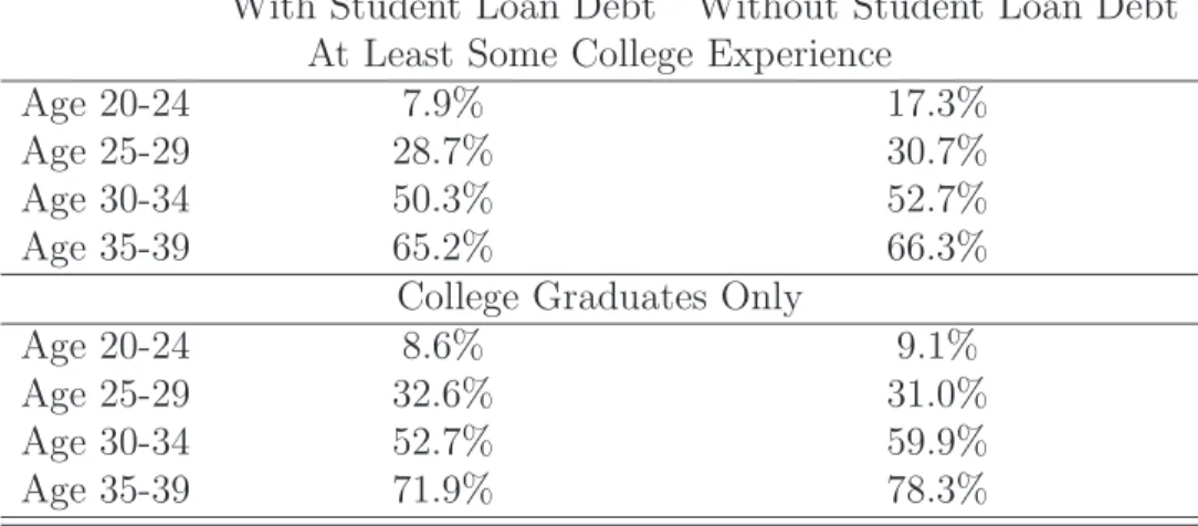
The top portion of Table1 shows homeownership rates, as of 2011, across age groups for households headed by an individual 39 years old or younger where at least one member (head or spouse) has at least some college experience.8 The homeownership rate for households with
student loan debt is always below the rate for households without student loan debt, with the widest differences observed for the youngest age group—those households with a head 20-to-24 years old. The homeownership rate gap for this age group is quite substantial, about
6
Note that owning a dwelling does not necessarily mean greater or better housing services than renting a dwelling. Nevertheless, there may be reasons to promote homeownership, and this is certainly a policy question that has received much attention.
7
It is possible that there are finer shades of difference among individuals who attended college but did not receive a degree depending on how many years they spent in college. We do not consider such distinctions because there is neither a clear theoretical case nor adequate data in the PSID.
8
9 percentage points. By comparison, the differences are much narrower for the next two age groups but still not trivial. For example, the homeownership rate for 30-to-34 year-olds is nearly 53 percent if they do not have outstanding student loan debt and only about 50 percent if they do. The homeownership rates appear to converge for 35-to-39 year-olds—the oldest age group in the sample we consider relevant—although the homeownership rate is still one percentage point lower for households with outstanding student debt.
This pattern of homeownership by age for households with at least some college experience seems to suggest that student loan debt delays households in purchasing a house but may not necessarily deter homeownership permanently. Note that we focus on households where the head is 39 years old or younger. As a result, we can be reasonably sure that the outstanding student loan debt was incurred by the head and/or spouse and is not student loan debt held by parents on behalf of their children. The pattern of relative homeownership rates, however, is similar if we extend the sample to older age groups (not shown).
The bottom portion of Table 1 shows homeownership rates when we restrict the sample to households where at least one family member (head or spouse) has a college degree. This restriction further refines our apples-to-apples comparison by not mixing college graduates with individuals who attended college but did not receive a degree. In principle, college graduates may be able to purchase a home more easily than college dropouts, and the two groups may also have different views about homeownership. The results show an interesting pattern: homeownership rates for college graduates who are 20-to-29 years old and have student loan debt are roughly the same as or higher than the rates for college graduates in this age range without student loan debt. In contrast, homeownership rates are a good bit lower for college graduates with debt who are older, specifically 30-to-39 years old, than the rates for peers without such debt.
A possible explanation for this pattern is that, among younger households with at least one college graduate, those who borrowed to fund their college education also have sufficiently
higher income that their expectations of life-time earnings net of student loan debt are also higher. These households are thus willing and able to purchase a property, In contrast, older households who still have student loan debt outstanding are likely to have experienced unfavorable realizations of income (relative to their expectations, on which they likely based their borrowing decisions) and are therefore less able to pay off their student debt or purchase a house. It is not clear why the pattern of relative homeownership rate across age groups differs between college graduates and those attended some college but did not receive a degree. Part of the reason may be the smaller sample size for college graduates in the PSID and thus the more pronounced difference for older households.
Overall, the two panels in Figure1show that the lower homeownership rate among student debt holders is not confined to those who borrowed to attend college but did not finish school. It is important to ask why student loan debt is associated with lower homeownership rates in the cross-section. One potential explanation is that households with student loan debt have more debt overall relative to income than households without student loan debt, all else being equal, making it more difficult for them to obtain additional credit. Alternatively, having a large student debt burden may make some households wary of taking on additional debt and thereby further increasing their debt service burden given their expected income in future years. We now turn to household balance-sheet and income data to conduct a preliminary analysis of these balance-sheet-based explanations.
Wealth Holdings
Figures 2 and 3 show the distribution of total wealth relative to income for homeowners and renters, respectively, who are 40 years old or younger. Total wealth (or equivalently household net worth) is the sum of a household’s financial assets and housing equity less any nonhousing liabilities.9 We average households’ wealth data in the 2011 and 2013 PSID to
9
obtain a smoothed measure of their holdings. Total (family) income data come from the 2011 wave.10 Households are further divided based on whether or not they had student loan debt
in 2011, and again the sample is restricted to those households where at least one member (head or spouse) has attended at least some college.
The distribution of total wealth relative to income (WY) for those households with stu-dent debt has a substantially lower mean than, and in fact lies mostly to the left of, the WY distribution for households without student debt (see Figure 2). This is true for both homeowners (left panel) and renters (right panel). Figure 3 shows that the distributions of total wealth relative to income are more closely aligned between households with and without student debt when wealth is computed without netting out student debt liabilities. This is especially the case for renters (right panel), where wealth holdings for households with stu-dent debt and households without stustu-dent debt are quite similar. This finding suggests that renters with student debt have lower wealth simply because of their student loan liabilities and not because of their inability (or lack of desire) to accumulate financial assets or increase their debt burden outside of student loans.
By comparison, a high percentage of homeowners with student debt have lower levels of total wealth relative to income than homeowners without student debt even without netting out their student debt liabilities. One plausible explanation for this discrepancy is that homeowners with student debt may not have been able to accumulate other assets as fast as homeowners without student debt because of their higher debt servicing costs. Given the wealth distributions for renters, however, it does not appear that student loan debt alone hinders household’s asset accumulation relative to income, unless there is something fundamentally different about homeowners and renters who carry student debt.
(IRA/401k) retirement accounts, business and/or farm, other real estate, and saving and other cash ac-counts. Housing equity is the value of one’s home less any outstanding mortgage debt.
10
Income data are not yet available in the 2013 PSID wave. Note as well that income is measured over the year prior to the PSID survey (for example, 2010 for the 2011 survey), while wealth is recorded in the PSID at the time a household is interviewed.
Tables 2 and 3 list key points in the distribution of total wealth holdings for households with and without student debt.11 Table 3 confirms that the distribution of total wealth
without netting out student loan liabilities (WOD) is similar for renters with and without student debt—especially in the bottom half of the distribution. Indeed, WOD holdings at the 25th and 50th percentiles are slightly higher for renters with student debt than for those without student debt, whereas renters with no student debt have greater wealth in the upper end of the WOD distribution. When student loan balances are netted against assets, however, total wealth is much lower for renters with student debt than for renters without student debt across the wealth distribution (see Table 2).
In addition, the amount of wealth held by homeowners with student debt is substantially lower than the amount of wealth held by homeowners without any student loan balances whether or not wealth holdings are calculated net of student loan liabilities (see Tables 2
and 3). These divergent wealth patterns between owners and renters continue to hold when wealth holdings are normalized by income (see TablesA.2andA.3in the appendix). In short, there appear to be systematic differences in wealth holdings for homeowners with outstanding student loan liabilities regardless of their income.
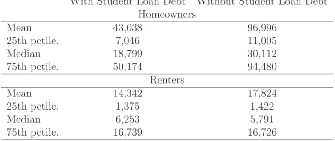
Tables4and5examine more disaggregated asset holdings for households with and without student loan debt. Table 4 shows that the wealth disparity for homeowners 40 years old and younger with and without student loans persists even in terms of financial wealth (wealth excluding housing equity). This result holds whether or not student loan debt is netted out in the calculation of financial wealth. The lower pace of wealth accumulation in general—both total and financial—by households with student debt may reflect these households’ greater debt service burden due to their student loan debt in addition to their mortgage debt.
In addition, cash holdings (assets held in checking and saving accounts) are noticeably lower for homeowners with student loan debt than for homeowners without student loan
11
Households with student debt are those households with student debt in 2011 and/or 2013. Households without student debt are households that reported no student loan liabilities in 2011 and 2013.
debt, while cash holdings for renters with student loan debt are higher than cash holdings for renters without student loan debt (see Table 5). This divergent pattern in cash holdings between homeowners and renters with student loan debt is broadly consistent with the idea that homeowners with student loan debt have not been able to keep as much of their income in liquid assets as homeowners without student loan liabilities. The fact that renters with student debt have greater cash holdings than renters without student debt could indicate that the former have better-paying jobs than their student-debt-free counterparts (due perhaps to their more expensive education that was financed with borrowing) and are thus able to save more of their income. Table 7 shows that renters with student debt indeed have higher pre-tax income than renters without student debt. Renters with student debt could also be stockpiling greater amounts of liquid assets than renters without student loan debt in order to meet the downpayment requirements for a future home purchase.
These finer distinctions notwithstanding, the question remains why in the cross section student debt liabilities are associated with substantially lower wealth holdings among home-owners. Do the explanations go beyond debt servicing costs, for both housing and student loan debt, which limit these households’ ability to save? Is it possible that individuals who had to borrow to attend college and possibly graduate schools are less well endowed either in aptitude or family background than their student-debt-free peers? Are these borrowers at a disadvantage in terms of life-time earnings and hence wealth holdings as well as home-ownership? Fully answering these questions is beyond the scope of this policy brief and our available data. Nevertheless, we explore a few possible explanations below.
First, we explore why homeowners with student loan debt also have higher balances of other forms of liabilities, such as credit card debt or loans from relatives. One reason these homeowners may have larger balances of overall nonhousing debt is that, after making payments on their mortgages, and housing-related expenses, they have to borrow more to cover their nonhousing expenses given where they are (40 years of age and younger) in their
lifetime earnings cycle. Another reason homeowners with student loan debt may borrow more in general is as part of an optimal life-cycle allocation: they may have higher expected future income but lower current income than homeowners without student loan debt.
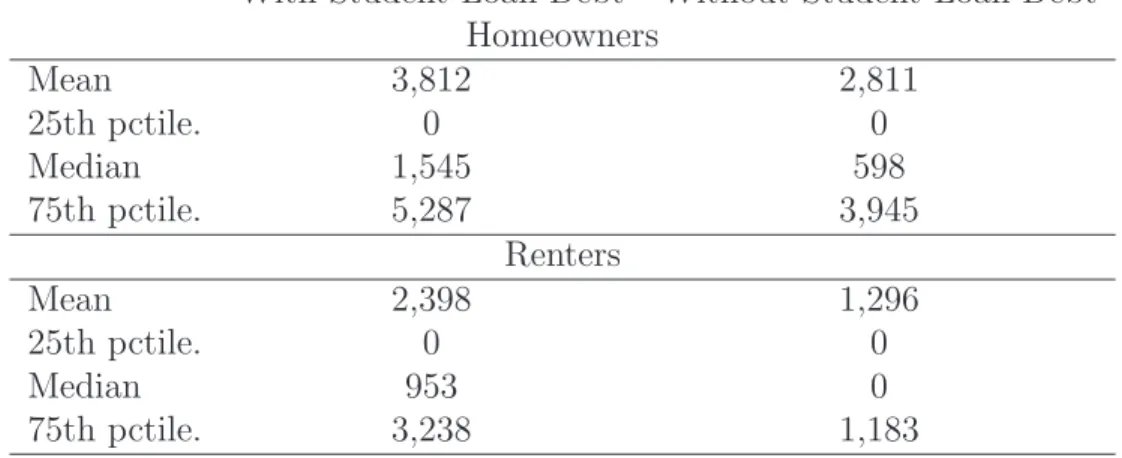
Unfortunately, we do not have enough information to estimate households’ expectations of future income. Instead, we compare the distribution of current (2010) family income and other (noncollateralized) debt holdings, respectively, for homeowners (and renters) who are 40 years old and younger. The results, reported in Tables 6 and 7, confirm that other debt outstanding is somewhat higher for households with student loan debt than for other house-holds, but the distribution of current income for homeowners is overall very similar between the two groups. These findings are inconsistent with households with student loan debt hav-ing lower current income than households without student loan debt, even though they do not rule out the possibility that the former group may expect to earn higher income in the future than the latter group. The results are at least suggestive, however, that homeowners with student loan debt may have accumulated greater overall debt balances than homeowners without student loan liabilities because they need to borrow more to finance nonhousing ex-penditures. Indeed, individuals and households with student loan debt have greater difficulty than others in obtaining nonhousing credit.
We next turn to regression analysis to better control for a host of additional characteristics that may differ systematically between homeowners with student loan debt and homeowners without student loan debt. For instance, homeowners without student loan debt may work in relatively better-paying industries or occupations and/or live in areas where housing is relatively more affordable. Also, those with student loan debt may be younger, on average, within the group of homeowners 40 years old and younger in our sample, and thus have had less time to accumulate wealth. Table 8 reports coefficient estimates from regressions that examine the conditional impact of student loan debt on WID for homeowners. Among other things, the regressions control for the age of the household head, the head’s industry and
occupation, whether he/she is married, the number of kids he/she has (if any), and location (state) fixed effects.12 The sample is restricted to homeowners 40 years old and younger,
where the household head (or spouse) has at least some college experience.
The first two columns of the table control for whether or not a household has any student loan debt, while the last two columns control for the amount of student debt (if any) on the household’s balance sheet. Columns (1) and (3) examine the impact of student loan debt on the log level of total wealth, while columns (2) and (4) examine the effect of student loan debt on household wealth relative to income.13 The results in Table 8 confirm that,
even conditional on other factors, homeowners with student loan debt have less wealth than homeowners without student loan debt. More specifically, the wealth of homeowners with student loan debt is considerably lower—roughly 0.9 log point lower—than the wealth of homeowners without student debt. These estimates capture the entirety of the effect of switching from not having student debt to having student debt on household wealth. The results in column (3) provide a better sense of the magnitude of the student debt effect by showing that a household’s dollar amount of student loan debt (in logs) affects its wealth, all else equal. In particular, we estimate that 10 percent higher student loan debt is associated with 0.9 percent lower total wealth holdings (without netting out student loan liabilities) for homeowners.
Consistent with the previous literature on socio-economic inequality in the United States, African Americans and Hispanics have substantially less wealth than Caucasians. This neg-ative effect is largely reversed, however, among those minority homeowners with student loan debt outstanding. This result likely reflects the fact that, among minorities, those who
12
We include a cubic term in the regressions for the age of the household head. 13
In order to avoid losing zero wealth observations we transform wealth using the inverse hyperbolic sine function following the approach in Dynan(2012). In particular,
wit=log h wit+ (wit+ 1) 1 2 i
wherewitis household wealth. According to Dynan (2012), this transformed variable can be interpreted the same way as a logarithmic variable, and thus we refer to it as “log wealth” for simplicity in our discussions.
pursued higher education—even if they had to borrow to do so—likely have greater earning power and can accumulate more assets while they are young than minorities who did not attend college. The coefficients in columns (1) and (3) also indicate that students who com-pleted college have higher wealth holdings than those who dropped out of college, but this advantage is diminished if a homeowner who completed college has student loan debt. The estimates using households’ wealth-to-income ratios as the dependent variable (see columns 2 and 4) tell a qualitatively similar story. Quantitatively, the direct effects of student loan debt on total wealth holdings are larger but lack precision. Restricting the sample to house-holds where the head (or spouse) has at least completed college also tell a similar story (See Appendix Table A.4). The estimated effects of student debt on wealth holdings are (not sur-prisingly) larger since this group of households spent more time in post-secondary education and thus likely had a greater need to borrow to pay for their schooling. Moreover, as a result of more years in school, these homeowners had fewer working years to earn income.
We cannot yet say that student loan debt causes lower asset accumulation among home-owners 40 years old and younger with at least some college education. However, the data do indicate that there is at least a strong negative correlation in the cross section between student loan debt and total wealth accumulation (net of student loan liabilities) among homeowners.
Impact of Student Debt on Homeownership (NELS88)
The final set of results uses data from the NELS88 to re-examine the relationship between stu-dent loan debt and future homeownership. As noted earlier, these data allow us to precisely control for whether an individual has ever borrowed to attend college as well as to control for an individual’s ability and educational and family characteristics. The period covered by the data enables us to examine the relationship between student debt and homeownership prior to the large run-up in aggregate student loan liabilities starting in the 2000s.
Table A.5 in the appendix shows summary statistics for our sample of individuals with at least some college experience compared with the full NELS88 sample in 2000. Aside from the education restriction necessary for our analysis, the two samples are quite similar along other dimensions. The homeownership rate and percentage of individuals who are married is slightly higher in our sample—a finding that is not surprising given that we have a more educated group of individuals. Overall, the evidence suggests that our restricted sample is representative of the overall (representative) NELS88 data outside of educational attainment. We analyze the relationship between homeownership and student debt using a linear probability model. Specifically, we regress an individual’s housing tenure status in 2000 (being a homeowner or not) on whether he/she had student loan debt or not as of 2000 and a number of controls.14 As robustness tests, we also consider whether the dollar amount
of an individual’s student debt, or student debt liabilities relative to income, impacts the probability of being a homeowner. One relevant control variable is the number of years since an individual finished school. Even though everyone in the NELS88 was in eighth grade in 1988, not everyone who went to college started at the same time, or dropped out or graduated at the same time. In fact, some individuals in the sample were still in college or graduate school as of 2000.
We expect the number of years since leaving school to be negatively correlated with the homeownership rate while perhaps positively correlated with the amount of student loan debt. The more recently an individual finished school, the less likely he/she is to have worked and settled down to the point of purchasing a home, regardless of his/her student debt liabilities. At the same time, the more time an individual spent in post-secondary education (which translates into fewer years since school in our sample), the more he/she likely needed to borrow to finance his/her education. On the other hand, it is possible that some individuals spent a longer time in college because they had to work part of the time to help pay for their
14
Logit estimates yield similar results. We focus on the linear probability estimates for ease of presentation and discussion.
education, and thus borrowed less than they would have otherwise.
We divide individuals into three “years since school” bins: 0-to-1 years, 2-to-4 years, and 5-to-8 years, and interact these bins with student debt holdings as well (0-to-1 years since is the excluded category).15 The interaction terms capture whether there is a differential
effect of student debt on homeownership based on the number of years since an individual finished (left) school. In particular, someone who has been out of school a short period of time and who has student loan debt may be particularly less likely to be a homeowner. We also control for an individual’s ability, which is likely correlated with his/her schooling choices and potentially homeownership, using a combined reading and math (standardized) test score based on aptitude tests administered as part of the NELS88 survey.16 In addition,
we include a (continuous) measure of the urbanicity of the zipcode that an individual lived in when the survey began in 1988, based on data from the 1990 U.S. Census.17 Including this
measure helps account for the fact that the type of location where an individual grew up may impact his/her educational opportunities as well as his/her propensity to be a homeowner or renter.
We also include an indicator for whether an individual worked in 1997 or 1998 yet was still enrolled in a post-secondary institution in 2000. This variable helps to capture individuals who returned to school after working and individuals who were attending school and working at the same time. These individuals may be quite different from those who reported being enrolled in school in 2000 as well as throughout the sample years. Other control variables include: an individual’s education level (some college [the excluded category], associate’s
15
Roughly 30 percent of the sample had been out of school 0-to-1 years, 30 percent had been out 2-to-4 years, and about 40 percent had been out 5-to-8 years.
16
The combined reading and math test score variable is a so-called t-score provided by the NELS88 as a continuous measure of an individual’s cognitive ability. It is an equal-weighted average of the standardized reading and math scores that is then re-standardized within a given year to have a mean of 50 and a standard deviation of 10. In this analysis, thet-score from 1992 was used.
17
We do not have direct data on whether an individual grew up in a rural or an urban area. Even if we had such a direct measure, it would ignore the fact that there is likely a gradation in the degree to which a location is urban or rural. The urbanicity of a zip code is calculated as the share of people living in urban areas within a zipcode.
degree, four-year degree, four-year degree but still in school),18 race, gender, family income
in 1987, parents’ education, the occupation and industry of the individual’s first job, his/her college major,19 and location (state) fixed effects, based on where he/she lived in 2000.
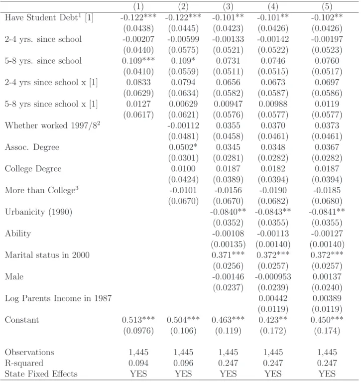
Table9shows our baseline estimates of the impact of student loan debt on homeownership using the NELS88 data. The regression reported in column 1 only includes the student debt indicator, controls for the number of years since the individual was in school, and state fixed effects.20 Note that the sample for these regressions is restricted to individuals who attended
at least some college. The estimates in column (1) show that individuals out of school 5-to-8 years are almost 11 percentage points more likely to own a home than individuals out only 0-to-1 years. Individuals out of school longer likely had more time to work and decide where to settle, as well as accumulate the necessary savings to purchase a home. The presence of student debt has a negative impact on homeownership of similar magnitude to being out of school 5-to-8 years. Specifically, individuals with student loan debt are 12 percentage points less likely to own a home than those without student loan debt. This effect is quite meaningful economically given that the homeownership rate for the sample is about 35 percent.
Interestingly, the relationship between student loan debt and homeownership is relatively invariant to the length of time someone has been out of school—the interaction effects are positive but imprecisely estimated. One might have expected that the debt effect would diminish with an individual’s number of years since school, as he/she has had time to repay some student debt. If anything, the effect of student loan debt on homeownership is weaker for someone out of school 2-to-4 years than for someone out 5-to-8 years, although these differences are insignificant. It may be the case that we do not observe differential effects of student loan debt based on the number of years since school because individuals in our
18
We assume that someone who has finished college but is still in school is likely still accruing student debt.
19
This control variable restricts the sample to those individuals who report their college major. 20
The excluded category is individuals either currently in school or who report they have been out of school up to one year.
sample have been out of school for a limited number of years overall.
The remaining columns of Table9show that the effect of student loan debt on homeowner-ship remains fairly constant when we add an increasing number of controls. The final column (column 5) includes not only controls for an individual’s industry, occupation, education level, and parents’ education, but also controls for the individual’s college major (if any).21 An
individual’s college major may help to capture his/her future earnings expectations beyond what is controlled for by the individual’s current industry and/or occupation.22 For instance,
an individual could be in a temporary job and hence temporary occupation/industry until he/she is able to find a position more consistent with his/her training (major) and/or career goals. Future earnings expectations are likely a relevant part of one’s homeownership decision; however, neither the industry and occupation controls nor the college major controls have much effect on the estimated relationship between student loan debt and homeownership.
The remaining analysis focuses on results using the full set of controls, including an individual’s college major. As in Table 9, however, our estimated effect of student loan debt is robust to the set of controls. Table 10shows results using alternative measures of student loan debt. For simplicity, only estimates for the main variables of interest are reported.23
Column 1 shows results using an individual’s (log) amount of student loan debt (if any). Again, there is a negative and precisely estimated relationship between homeownership and student loan debt that does not vary much based on the number of years an individual has been out of school. The estimates suggest that 10 percent higher student loan debt relative
21
We recognize that there may be aspects of parental influence, such as the attitude toward homeownership, that is not fully captured by parents’ education or income. But there is no obvious reason to suspect that these are correlated with student debt.
22
The categories we use for college major are: Category 1: math and sciences; Category 2: language, literature, philosophy, religion, and ethnic studies; Category 3: accounting, finance, business, and market-ing; Category 4: tech/computer-related, programming, and engineermarket-ing; Category 5: education; Category 6: health-related; Category 7: home economics, secretarial, consumer service; Category 8: law; Category 9: liberal studies; Category 10: protective services, social work; Category 11: social sciences, communica-tions; Category 12: construction, mechanics, precision production, and transportation; Category 13: art and architecture.
23
to the mean leads to a 0.1 percentage point lower likelihood of homeownership.
It is possible, however, that what really matters for homeownership is not the absolute amount of an individual’s outstanding student loan debt but rather his/her student loan debt relative to his/her current income. This ratio is perhaps a better proxy for the burden of an individual’s debt relative to his/her current cash flow (that is, the debt service ratio). Individuals with a large share of current income going to service their student loan debt may have a more difficult time obtaining a mortgage loan than individuals whose student loan liabilities are relatively small compared with their cash flow. Column 2 in Table 10
shows estimates using individuals’ student debt-relative-to-income (SDY) as the primary explanatory variable. The results show that indeed individuals whose cash flow is particularly burdened by student loan debt are less likely to own a home—especially those individuals who have been out of school 5-to-8 years. This finding contrasts with our earlier results that used other measures of student debt and showed little evidence of a differential effect of student loan debt depending on how long someone had been out of school. One plausible explanation is that the previous regressions did not control for an individual’s income directly, and broad-based controls of one’s industry, occupation, or even college major are too imprecise to capture the differences across individuals in terms of their debt service capacity.24
The results are broadly similar when we restrict the sample to individuals with posi-tive student loan debt only (columns 3 and 4). The impact of (log) student loan debt on homeownership is more than five times larger (in absolute value) given this restriction than with the full sample, but the estimate is imprecise. A 1 percent increase in student loan debt, lowers homeownership by 5.6 percentage points. In addition, the interactions between SDY and years since school are smaller and less precisely estimated (column 4). This lack of precision is not surprising since the sample size dropped a good deal with the positive-debt restriction. Overall, these results reinforce the conclusion that there is a non-negligible
24
The effect captured by our debt service capacity measure may reflect both the individual’s own reluctance to take on housing debt (demand effect) and lenders’ reluctance to extend credit (supply effect).
negative correlation between student debt balances and homeownership among the NELS88 survey respondents—at least as of 2000 when they were last surveyed.
5
Conclusion
This study examines if and how having student loan debt outstanding affects an individual’s other economic outcomes. Compared with the existing literature on student debt that mostly uses credit bureau data, this paper employs alternative data that, while smaller in sample size, contains a much richer set of demographic and financial information for individuals in addition to their student debt liabilities. These data allow us to make careful “apples-to-apples” comparisons between individuals with truly comparable attributes, especially whether or not they have at least some college experience.
We find that, in the cross section, having student debt outstanding is associated with a lower rate of homeownership as well as with lower wealth holdings. The negative effect of student loan debt on wealth holdings is more pronounced among homeowners than among renters. These negative correlations are robust to controlling for many observable factors that likely also impact homeownership and wealth accumulation. Household balance-sheet data suggest that the lower wealth accumulation among homeowners with outstanding student debt is likely due to greater expenses for these households rather than to lower income. We cannot, however, yet conclude that student debt causes lower homeownership rates and wealth. A more structural approach along with better data are needed to assess whether there is a causal link.
More broadly, additional research is needed to better understand why student loan lia-bilities seem to be associated with worse economic outcomes for individuals and households. A plausible explanation is that, among households whose members have attended at least some years of college, those with student debt are more burdened by their debt service costs
than those with no student debt. This greater debt burden limits their ability to save and/or invest. On the other hand, it is also possible that, compared with individuals without out-standing student debt, those who do have a steeper life-cycle earnings profile tend to have lower homeownership rates along with less wealth in their 20s and 30s since they expect to catch up later in life with higher income. Ultimately, what we care about is whether those in-dividuals who have borrowed to attend college would have been better off pursuing less costly alternative forms of education or training after high school. Therefore, much more work is needed to determine whether individuals and households are making optimal decisions in terms of financing their education with student borrowing.
References
Brown, Meta, and Sydnee Caldwell. 2013. “Young Student Loan Borrow-ers Retreat from Housing and Auto Markets.” Liberty Street Economics
Available at: http://libertystreeteconomics.newyorkfed.org/2013/04/young-student-loan-borrowers-retreat-from-housing-and-auto-markets.html#.VCr0AhYgubM (last accessed 9/30/2014).
Brown, Meta, Andrew Haughwout, Donghoon Lee, Maricar Mabutas, and Wilbert van der Klaauw. 2012. “Grading Student Loans.” Liberty Street Economics Available at: http://libertystreeteconomics.newyorkfed.org/2012/03/grading-student-loans.html#. VCr1DBYgubM (last accessed 9/30/2014).
Brown, Meta, Andrew Haughwout, Donghoon Lee, Joelle Scally, and Wilbert van der Klaauw. 2014. “Measuring Student Debt and Its Performance.” Staff report no. 668. New York, NY: Federal Reserve Bank of New York.
Carneiro, Pedro, James J. Heckman, and Edward J. Vytlacil. 2010. “Estimating Marginal Returns to Education.” Working paper 16474. Cambridge, MA: National Bureau of Eco-nomic Research.
Dynan, Karen. 2012. “Is a Household Debt Overhang Holding Back Consumption?” Brook-ings Papers on Economic Activity Spring.
Houle, Jason, and Lawrence Berger. 2014. “Is Student Loan Debt Discouraging Home Buying Among Young Adults?” mimeo. Hanover, NH: Dartmouth College.
Ionescu, Felicia. 2012. “The Federal Student Loan Program: Quantitative Implications for College Enrollment and Default Rates.” Review of Economic Dynamics 12: 205–231.
Figure 1 0 200 400 600 800 1000 1200 Billions of Dollars 2004q1 2006q1 2008q1 2010q1 2012q1 2014q1
HELOC Auto Loan
Credit Card Student Loan
Source: New York Fed Consumer Credit Panel / Equifax
Nonmortgage Balances
Figure 2 0 5 10 15 Percent −3 −2 −1 0 1 2 3 4 5 6 Total Wealth / Family IncomeWith Student Loan Debt Without Any Student Loan Debt
Source: Panel Study of Income Dynamics, public use dataset.
Note: Total Wealth is the average of 2011 and 2013 wealth. The sample is restricted to households where either the head or the spouse has at least some college experience.
The top and bottom 2% of the data are trimmed, and the data are winsorized at an upper bound of 6.
without netting out student loan debt from total wealth calculations
Distribution of Total Wealth relative to Income for Homeowners 40 or Younger
0 5 10 15 20 Percent −3 −2 −1 0 1 2 3
Total Wealth / Family Income With Student Loan Debt Without Any Student Loan Debt
Source: Panel Study of Income Dynamics, public use dataset.
Note: Total Wealth is the average of 2011 and 2013 wealth. The sample is restricted to households where either the head or the spouse has at least some college experience.
The top and bottom 2% of the data are trimmedm and the data are winsorized at an upper bound of 3.
Figure 3 0 5 10 15 Percent −2 0 2 4 6
Total Wealth / Family Income With Student Loan Debt Without Any Student Loan Debt
Source: Panel Study of Income Dynamics, public use dataset.
Note: Total Wealth is the average of 2011 and 2013 wealth. The sample is restricted to households where either the head or the spouse has at least some college experience.
The top and bottom 2% of the data are trimmed, and the data are winsorized at an upper bound of 6.
without netting out student loan debt from total wealth calculations
Distribution of Total Wealth relative to Income for Homeowners 40 or Younger
0 5 10 15 20 Percent −1 0 1 2 3
Total Wealth / Family Income With Student Loan Debt Without Any Student Loan Debt
Source: Panel Study of Income Dynamics, public use dataset.
Note: Total Wealth is the average of 2011 and 2013 wealth. The sample is restricted to households where either the head or the spouse has at least some college experience.
The top and bottom 2% of the data are trimmed, and the data are winsorized at an upper bound of 3.
without netting out student loan debt from total wealth calculations
Table 1: Homeownership Rate by Age Group
With Student Loan Debt Without Student Loan Debt At Least Some College Experience
Age 20-24 7.9% 17.3% Age 25-29 28.7% 30.7% Age 30-34 50.3% 52.7% Age 35-39 65.2% 66.3%
College Graduates Only
Age 20-24 8.6% 9.1%
Age 25-29 32.6% 31.0% Age 30-34 52.7% 59.9% Age 35-39 71.9% 78.3%
Source: Authors’ calculations using PSID data. Notes: Data on the presence or absence of student loan debt refer to 2011 and/or 2013. The top portion of the table is restricted to households where the head or spouse (or both) have at least some college experience. The bottom portion of the table is restricted to households where the head or spouse (or both) have a college degree or more.
Table 2: Distribution of Real Total Wealth
With Student Loan Debt Without Student Loan Debt Homeowners Mean 51,435 158,593 25th pctile. -786 27,752 Median 25,667 76,674 75th pctile. 71,308 173,684 Renters Mean -4,734 19,915 25th pctile. -18,999 1,520 Median -5,298 5,830 75th pctile. 5,312 18,863
Source: Authors’ calculations using PSID data. Notes: Data on the presence or absence of student loan debt refer to 2011 and/or 2013. Wealth is the sum of financial assets and housing assets less any outstanding debt. Wealth data are deflated using the PCE deflator (2000 base year) and averaged over 2011 and 2013. The sample is restricted to households where the head is 40 years old or younger and at least one member of the household (head or spouse) attended some college.
Table 3: Distribution of Real Total Wealth
Without Netting Out Student Loan Liabilities
With Student Loan Debt Without Student Loan Debt Homeowners Mean 72957 158593 25th pctile. 19429 27752 Median 43066 76674 75th pctile. 91293 173684 Renters Mean 16829 19915 25th pctile. 1890 1520 Median 7100 5830 75th pctile. 19906 18863
Source: Authors’ calculations using PSID data. Notes: Data on the presence or absence of student loan debt refer to 2011 and/or 2013. Wealth is the sum of financial assets and housing assets less any outstanding debt except student loans. Wealth data are deflated using the PCE deflator (2000 base year) and averaged over 2011 and 2013. The sample is restricted to households where the head is 40 years old or younger and at least one member of the household (head or spouse) attended some college.
Table 4: Distribution of Real Financial Wealth
Without Netting Out Student Loan Liabilities
With Student Loan Debt Without Student Loan Debt Homeowners Mean 43,038 96,996 25th pctile. 7,046 11,005 Median 18,799 30,112 75th pctile. 50,174 94,480 Renters Mean 14,342 17,824 25th pctile. 1,375 1,422 Median 6,253 5,791 75th pctile. 16,739 16,726
Source: Authors’ calculations using PSID data. Notes: Data on the presence or absence of student loan debt refer to 2011 and/or 2013. Financial wealth is the sum of financial assets less any outstanding nonhousing debt except student loans. Wealth data are deflated using the PCE deflator (2000 base year) and averaged over 2011 and 2013. The sample is restricted to households where the head is 40 years old or younger and at least one member of the household (head or spouse) attended some college.
Table 5: Distribution of Real Cash Holdings
With Student Loan Debt Without Student Loan Debt Homeowners Mean 6,925 13,837 25th pctile. 1,087 1,535 Median 3,299 4,690 75th pctile. 7,889 14,325 Renters Mean 3,413 3,255 25th pctile. 192 0.77 Median 1,201 789 75th pctile. 3,945 3,156
Source: Authors’ calculations using PSID data. Notes: Data on the presence or absence of student loan debt refer to 2011 and/or 2013. Cash is the sum assets in checking and savings accounts. The data are deflated using the PCE deflator (2000 base year) and averaged over 2011 and 2013. The sample is restricted to households where the head is 40 years old or younger and at least one member of the household (head or spouse) attended some college.
Table 6: Distribution of Real Nonhousing Debt
Other than Student Loan Debt
With Student Loan Debt Without Student Loan Debt Homeowners Mean 3,812 2,811 25th pctile. 0 0 Median 1,545 598 75th pctile. 5,287 3,945 Renters Mean 2,398 1,296 25th pctile. 0 0 Median 953 0 75th pctile. 3,238 1,183
Source: Authors’ calculations using PSID data. Notes: Data on the presence or absence of student loan debt refer to 2011 and/or 2013. Nonhousing debt includes credit card debt, loan from relatives, and other noncollateralized debt except student loans. The data are deflated using the PCE deflator (2000 base year) and are averaged over 2011 and 2013. The sample is restricted to households where the head is 40 years old or younger and at least one member of the household (head or spouse) attended some college.
Table 7: Distribution of Real Pre-Tax Family Income
With Student Loan Debt Without Student Loan Debt Homeowners Mean 66,997 70,836 25th pctile. 43,902 42,681 Median 61,174 63,114 75th pctile. 83,784 90,016 Renters Mean 37,083 33,091 25th pctile. 18,540 17,357 Median 31,557 29,979 75th pctile. 50,135 44,862
Source: Authors’ calculations using PSID data. Notes: Data on the presence or absence of student loan debt refer to 2011 and/or 2013. Income is total family income for 2010 (2011 PSID Survey) The data are deflated using the PCE deflator (2000 base year). The sample is restricted to households where the head is 40 years old or younger and at least one member of the household (head or spouse) attended some college.
Table 8: Impact of Student Loan Debt on Household Wealth
(1) (2) (3) (4) Have Student Debt1 [1] -0.907* -1.084*
(0.472) (0.617)
Log Student Debt [2] -0.0850* -0.0922 (0.0448) (0.0582) Black -1.675*** -1.792** -1.658*** -1.733** (0.534) (0.859) (0.531) (0.855) Black x [1] 0.689 1.262* (0.641) (0.669) Black x [2] 0.0634 0.107* (0.0583) (0.0614) College Degree or more 1.399*** 0.357 1.409*** 0.353
(0.446) (0.602) (0.440) (0.592) College Degree or more x [1] -0.381 0.0788
(0.555) (0.627)
College Degree or more x [2] -0.0330 0.00823 (0.0513) (0.0581) Married 0.676** -0.0506 0.688** -0.0478
(0.333) (0.273) (0.333) (0.275) Log Family Income 1.483*** 1.479***
(0.201) (0.201)
Constant 4.512 -17.85 3.865 -18.60 (21.35) (23.78) (21.38) (24.01)
Observations 2,206 2,206 2,206 2,206 R-squared 0.156 0.042 0.156 0.041 Industry Fixed Effect YES YES YES YES Occupation Fixed Effect YES YES YES YES State Fixed Effect YES YES YES YES
Source: Authors’ calculations using PSID data. Notes: 1
Indicator variable that takes a value of 1 if the household has outstanding student debt liabilities in 2011 and/or 2013 and is zero otherwise. The sample is restricted to households where the head is 40 years old or younger and at least one member of the household (head or spouse) has at least some college experience. The dependent variable in columns (1) and (3) is the log of households’ total wealth without netting out student loan debt. The mean of this variable is 8.2 with a standard deviation of 6.6. The dependent variable in columns (2) and (4) is total wealth relative to income. The mean of this variable is 1.33 with a standard deviation of 6.5. Wealth is the sum of financial assets and housing assets less any outstanding debt except student loans. Wealth data in columns (1) and (3) are deflated using the PCE deflator (2000 base year) and averaged over 2011 and 2013. Income is total family income for 2010 (2011 PSID Survey). Other data are deflated using the PCE deflator (2000 base year) where applicable. Estimates also include age, age squared, and age cubed for the household head and a variable for the number of children in the household. Robust standard errors are in parentheses: *** p<0.01, ** p<0.05, * p<0.1
Table 9: Student Loan Debt and Homeownership
(1) (2) (3) (4) (5) Have Student Debt1 [1] -0.122*** -0.122*** -0.101** -0.101** -0.102**
(0.0438) (0.0445) (0.0423) (0.0426) (0.0426) 2-4 yrs. since school -0.00207 -0.00599 -0.00133 -0.00142 -0.00197 (0.0440) (0.0575) (0.0521) (0.0522) (0.0523) 5-8 yrs. since school 0.109*** 0.109* 0.0731 0.0746 0.0760
(0.0410) (0.0559) (0.0511) (0.0515) (0.0517) 2-4 yrs since school x [1] 0.0833 0.0794 0.0656 0.0673 0.0697
(0.0629) (0.0634) (0.0582) (0.0587) (0.0586) 5-8 yrs since school x [1] 0.0127 0.00629 0.00947 0.00988 0.0119
(0.0617) (0.0621) (0.0576) (0.0577) (0.0577) Whether worked 1997/82 -0.00112 0.0355 0.0370 0.0373 (0.0481) (0.0458) (0.0461) (0.0461) Assoc. Degree 0.0502* 0.0345 0.0348 0.0367 (0.0301) (0.0281) (0.0282) (0.0282) College Degree 0.0100 0.0187 0.0182 0.0187 (0.0424) (0.0389) (0.0394) (0.0394) More than College3 -0.0101 -0.0156 -0.0190 -0.0185
(0.0670) (0.0670) (0.0682) (0.0680) Urbanicity (1990) -0.0840** -0.0843** -0.0841** (0.0352) (0.0355) (0.0355) Ability -0.00108 -0.00113 -0.00127 (0.00135) (0.00140) (0.00140) Marital status in 2000 0.371*** 0.372*** 0.372*** (0.0256) (0.0257) (0.0257) Male -0.00146 -0.000953 0.00137 (0.0237) (0.0239) (0.0240) Log Parents Income in 1987 0.00442 0.00389
(0.0119) (0.0119) Constant 0.513*** 0.504*** 0.463*** 0.423** 0.450*** (0.0976) (0.106) (0.119) (0.172) (0.174)
Observations 1,445 1,445 1,445 1,445 1,445 R-squared 0.094 0.096 0.247 0.247 0.247 State Fixed Effects YES YES YES YES YES
Source: Authors’ calculations using NELS88 data. Notes: 1
Indicator variable that takes a value of 1 if the individual has outstanding student debt liabilities in 2000 and is zero otherwise. 2
Indicator variable that takes a value of 1 if the individual reports working in 1997 and/or 1998. 3
Individuals who finish college and report that they are still in school in 2000. The sample is restricted to individuals who at least attended some college. The dependent variable is an indicator variable that takes a value of 1 if the individual is a homeowner in 2000 and is 0 otherwise. Ability is measured based on a combined standardized reading and math score. Parental income in 1987 is a categorical variable and parents are assigned the midpoint of their respective income category. Industry and occupation of the individual’s first job are omitted from the table, but are controlled for in columns (3),(4), and (5). Columns (3), (4), and (5) also control for the individual’s race. Parental education level is controlled for in columns (4), and (5). College major is controlled for in column (5). Robust standard errors are in parentheses: *** p<0.01, ** p<0.05, * p<0.1
Table 10: Student Loans and Homeownership (OLS)
(1) (2) (3) (4) Log Student Debt [1] -0.0110*** -0.0557
(0.00422) (0.0392)
Student Debt rel. Income [2] -0.0109 -0.00669 (0.00740) (0.00710) 2-4 yrs. since school -0.00182 0.0351 0.198 0.141**
(0.0521) (0.0477) (0.511) (0.0665) 5-8 yrs. since school 0.0755 0.111** 0.445 0.169**
(0.0516) (0.0496) (0.575) (0.0770) 2-4 yrs. since school x [1] 0.00681 -0.00662
(0.00585) (0.0513) 5-8 yrs. since school x [1] 0.000264 -0.0344
(0.00603) (0.0603)
2-4 yrs. since school x [2] -0.0264** -0.0215 (0.0131) (0.0143) 5-8 yrs. since school x [2] -0.202*** -0.0910
(0.0661) (0.0884) Constant 0.453*** 0.434** 0.375 -0.327
(0.174) (0.191) (0.494) (0.319)
Observations 1,445 1,297 594 528 R-squared 0.248 0.245 0.252 0.251 State Fixed Effects YES YES YES YES
Source: Authors’ calculations using NELS88 data. Notes: The sample is restricted to individuals who at least attended some college. Columns (3) and (4) are further restricted to respondents with positive student loan debt. The dependent variable is an indicator variable that takes a value of 1 if the individual was a homeowner in 2000 and is 0 otherwise. Additional controls in all columns include: an individual’s employment status in 1997 or 1998, education level, high school test scores, race, sex, industry and occupation of his/her first job, marital status, and college major, as well as the urbanicity of the zipcode in which the individual lived in 1988, parental education and income (1987) controls, level dummies, household’s income in 1987. Robust standard errors are in parentheses: *** p<0.01, ** p<0.05, * p<0.1
A
Appendix
Table A.1: Sample Size for Each Age Group in Figure 2
With Student Loan Debt Without Student Loan Debt At Least Some College Experience
Age 20-24 127 127
Age 25-29 373 261
Age 30-34 336 334
Age 35-39 221 276
Age 40-44 133 301
College Graduates Only
Age 20-24 61 35
Age 25-29 222 109
Age 30-34 207 135
Age 35-39 124 119
Age 40-44 87 151
Source: Authors’ calculations using PSID data. Notes: Data on the presence or absence of student loan debt refer to 2011 and/or 2013.
Table A.2: Distribution of Total Wealth-to-Income
With Student Loan Debt Without Student Loan Debt Homeowners Mean 0.73 2.15 25th pctile. -0.04 0.56 Median 0.45 1.27 75th pctile. 1.20 2.31 Renters Mean -0.37 0.58 25th pctile. -0.79 0.06 Median -0.17 0.22 75th pctile. 0.15 0.59
Source: Authors’ calculations using PSID data. Notes: Data on the presence or absence of student loan debt refer to 2011 and/or 2013. Total wealth is the sum of financial assets and housing assets less any outstanding debt. These data are averaged over 2011 and 2013. Income is total family income in 2010 (2011 survey). The sample is restricted to households where the head is 40 years old or younger
Table A.3: Distribution of Total Wealth-to-Income
Without Netting out Student Loan Debt
With Student Loan Debt Without Student Loan Debt Homeowners Mean 1.09 2.07 25th pctile. 0.35 0.54 Median 0.72 1.23 75th pctile. 1.44 2.31 Renters Mean 0.44 0.56 25th pctile. 0.06 0.06 Median 0.24 0.22 75th pctile. 0.56 0.56
Source: Authors’ calculations using PSID data. Notes: Data on the presence or absence of student loan debt refer to 2011 and/or 2013. Total wealth is the sum of financial assets and housing assets less any outstanding debt except student debt. These data are averaged over 2011 and 2013. Income is total family income in 2010 (2011 survey). The sample is restricted to households where the head is 40 years old or younger
Table A.4: Impact of Student Loan Debt on Household Wealth
(1) (2) (3) (4) Have Student Debt1 [1] -1.459*** -1.024***
(0.406) (0.354)
Log Student Debt [2] -0.139*** -0.0878** (0.0369) (0.0356) Black -2.593** -1.724*** -2.728** -1.754*** (1.093) (0.495) (1.075) (0.515) Black x [1] 1.290 1.072* (1.184) (0.584) Black x [2] 0.134 0.0988* (0.101) (0.0518) Married 1.039** 0.126 1.054** 0.130 (0.468) (0.347) (0.468) (0.348) Log family income 1.441*** 1.428***
(0.296) (0.296)
Constant -6.313 15.18 -6.827 15.23 (43.68) (21.15) (43.54) (21.05)
Observations 1,026 1,026 1,026 1,026 R-squared 0.158 0.103 0.159 0.102 Industry Fixed Effect YES YES YES YES Occupation Fixed Effect YES YES YES YES State Fixed Effect YES YES YES YES
Source: Authors’ calculations using PSID data. Notes: 1
Indicator variable that takes a value of 1 if the household has outstanding student debt liabilities in 2011 and/or 2013 and is zero otherwise. Wealth is the sum of financial assets and housing assets less any outstanding debt except student loans. The sample is restricted to households where the head is 40 years old or younger and at least one member of the household (head or spouse) has completed college. The dependent variable in columns (1) and (3) is the log of households’ total wealth without netting out student loan debt. The mean of this variable is 9.5 with a standard deviation of 5.9. The dependent variable in columns (2) and (4) is total wealth relative to income. The mean of this variable is 1.5 with a standard deviation of 4.6. Wealth data in columns (1) and (3) are deflated using the PCE deflator (2000 base year) and averaged over 2011 and 2013. Income is total family income for 2010 (2011 PSID Survey). Other data are deflated using the PCE deflator (2000 base year) where applicable. Estimates also include age, age squared, and age cubed for the household head and a variable for the number of children in the household. Robust standard errors are in parentheses: *** p<0.01, ** p<0.05, * p<0.1