Software Fault Prediction Using Filtering Feature
Selection in Cluster-Based Classification
Fachrul Pralienka Bani Muhamad
1, Daniel Oranova Siahaan
2, Chastine Fatichah
2 Abstract―The high accuracy of software fault prediction canhelp testing effort and improving software quality. Previous researchers had proposed the combination of Entropy-Based Discretization (EBD) and Cluster-Based Classification (CBC). However, the irrelevant and redundant features in software fault dataset tend to decrease the prediction accuracy value. This study proposes improvement of CBC outcomes by integrating filtering feature selection methods. Filtering feature selection methods that will be integrated with CBC i.e. Information Gain (IG), Gain Ratio (GR), and One-R (OR). Based on the research using 2 datasets NASA public MDP (i.e. PC2 and PC3), the result shows that the combination of CBC and IG yields the best average accuracy value compared to GR and OR. It generates 67.52% average of probability detection (pd) and 37.42% average of probability false alarm (pf). While CBC without feature selection yields 65.38% average pd and 49.95% average pf. It can be concluded that IG can improve CBC outcomes by increasing 2.14% average pd and reducing 12.53% average pf.
Keywords―Cluster-based Classification, Entropy-Based
Discretization, Filtering Feature Selections, Software Fault Prediction.
I. INTRODUCTION1
Software fault prediction is very important to do, because the allocation of cost and testing resources are limited. In addition, software fault prediction can make testing process focus on fault-prone modules, so that test resources can be saved for other faulty-prone modules. Software fault prediction is the most efficient quality assurance activity, as it can reduce testing time by saving test resources [1].
Previous researchers have proposed several methods to predict software fault, i.e. Genetic Programming, Decision Tree, Neural Network, Density-based Clustering, Case-based Reasoning, Fuzzy Logic, Logistic Regression, and Naive Bayes [2]. In general, methods that can produce high predictive values tend to use a simple modeling technique i.e. Naive Bayes [3]. Naïve Bayes (NB) can generate about 71% probability detection (pd) and 25% probability false alarm (pf) in 8 datasets of NASA public MDP [4]. When NB compared to the Cluster-based Classification (CBC) [2], then CBC can produce better predictive result, i.e. 83.3% pd and 40% pf in 7 datasets of NASA public MDP.
1Fachrul Pralienka Bani Muhamad is with Department of Informatics Engineering, Polytechnic of Indramayu, Indramayu 45252, Indonesia. E-mail: [email protected].
2Daniel Oranova Siahaan, Chastine Fatichah are with Department of Informatics Engineering, Faculty of Information Technology, Institut Teknologi Sepuluh Nopember (ITS), Kampus ITS Sukolilo, Surabaya 60111, Indonesia. E-mail: [email protected];[email protected].
However, some researchers have described that predictive models with irrelevant features as well as redundant features can generate lower predictive values. In previous research [5], filtering feature selection methods were used to improve NB result in predicting software fault using Turkish white-goods manufacturer datasets. Filtering feature selection methods used in the previous research were Gain Ratio (GR), Information Gain (IG), and One-R (OR). The result shows that the combination of NB and OR can yield the highest prediction accuracy value compared to NB and IG, NB and GR, and NB without feature selection.
This study is proposed to improve CBC prediction values by using three methods of filtering features selection i.e. GR, IG, and OR. From that combinations, an analysis will be performed to find the best combination of CBC which can generate the highest pd and the lowest pf, and the best number of features used as input in CBC. The experiment was performed in 2 datasets NASA public MDP i.e. PC2 and PC3. The combination of CBC and filtering feature selection methods are expected to improve software fault prediction result.
II. LITERATURE REVIEW
This chapter is described about related research on software fault prediction. In addition, there are also a description of software fault, NASA public MDP dataset, and basic supporting theories. The basic theories used in this chapter are entropy-based discretization (EBD), filtering feature selection (GR, IG, OR), and cluster-based discretization (CBC).
A. Previous Research
Systematic literature review by [6], [7], and [1] that discuss about finding solution on software fault prediction. The results show that solution by statistical method for predicting software fault has started to be abandoned, while the research area using data mining to predict software fault is the most popular. This is due to the wide variety of methods in data mining to improve the accuracy of software fault predictions. Data mining methods that can produce high prediction accuracy tend to use simple methods, such as NB.
[4] was proposed a NB method for predicting software fault. The proposed method is applied to 8 NASA public MDP datasets by performing a log number preprocess combined with IG feature selection method. The results showed values of 71% pd and 25% pf.
[8] proves that the classification of k-NN with discretization of numerical data using EBD in preprocess
can improve prediction accuracy. This is supported by hand geometry datasets that contain numerical data. In addition, the EBD method can reduce the possibility of over-fitting prediction models and process predictions more rapidly than continuous (numeric) data.
[9] have tried a combination of NB with a preprocess EBD on two embedded software system fault datasets obtained from NASA's public MDP. The results show that EBD can help improve the accuracy of NB in predicting software fault. This study also proves that the characteristics of several embedded software system datasets on NASA public MDP are suitable for discretization with EBD.
[10] and [11] propose a CBC method for predicting software faults. The first study combines CBC with EBD on three software fault datasets obtained from Turkish white good manufacturer Software Company. The results show that the accuracy of the CBC method with EBD is superior to the ANN method. While the second study did the same with the first study, but with the dataset used more diverse i.e. 7 datasets of software fault from NASA public MDP. The results showed that CBC and EBD yielded a higher degree of accuracy when compared to NB which previously tended to produce high accuracy values. The pd value increases to 83% and the pf value becomes 40%.
[12] used a feature selection method to improve predicted accuracy results in NB. The study was conducted on the Turkish software industry dataset. The results showed that the OR feature selection method yielded the best value compared to the other four selection methods of IG, GR, RFF, and SU.
[13] proposes a combination of NB methods with GR. The results show that the accuracy of software fault prediction on NASA public MDP dataset can be enhanced by the selection of GR features. To support a cooperative NB method on discrete data, the software fault data is first discretized into five categories at random point.
[14] examines the effect of feature selection on the NB prediction model. The researcher uses five datasets obtained from UCI repository namely mushroom. Some feature selection methods that are integrated with NB are IG, GR, SU, OR, RFF, and chi-squared (CS). The results show that OR is the highest feature selection method in improving the accuracy of the NB method of classification. B. Software Fault
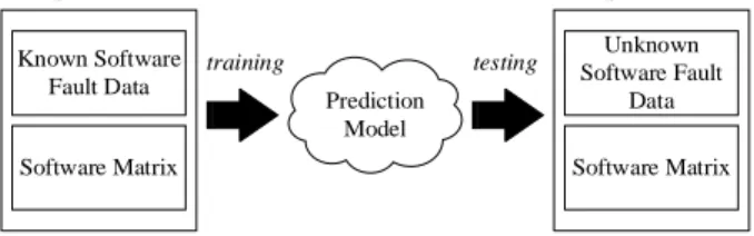
Software fault are a major problem in software systems that need to be minimized to ensure it reliability [15]. Any software fault can always be observed during the testing process. Software fault can lead to software failures resulting in increased costs and attempts to correct the fault. Software failure signifies the low level of quality of the software. To improve the software quality level, software fault need to be minimized. The prediction of software fault is the predictability of fault-prone modules in the next release stage by using prediction metrics and software fault data in previous versions. In general, the prediction process of software fault can be seen in figure1.
Prediction Model Known Software Fault Data Software Matrix Unknown Software Fault Data Software Matrix Previous Version of Software
The Latest Version of Software
training testing
Figure 1. Software fault prediction. C. Nasa Public MDP Dataset
Software fault prediction is one of the important factors in improving quality in software development process. As mentioned earlier, that to predict software fault required some metrics and software fault data from previous software versions. The software metrics is a simple quantitative measure of each attribute in the software lifecycle. The software metrics allows researchers to measure and predict software processes, required resources, and work products relevant to software development efforts. Software metrics often used by researchers to measure the complexity of program code are line of code (loc), mcCabe complexity, and halstead complexity [9].
Various datasets containing metric variations have been used to predict software fault, and some are private. Due to the lack of access to use private datasets, this research will utilize public datasets that can be accessed by all researchers and can be used for various purposes. One of the most commonly researched software fault datasets is the NASA public MDP. The dataset can be generally accessed through the repository of the promise software engineering dataset. NASA public MDP dataset generally contains numerical data type consist of line of code, mcCabe complexity, halstead complexity, and software fault labels [16].
D. Entropy-Based Discretization (EBD)
Data mining methods have been successfully applied to solve predictions or classification problems on various background issues. In data mining, the discrete process is known as one of the most important preprocess data activities. Most algorithms on data mining methods are able to extract knowledge from datasets with features that contain discrete data. If the data on the dataset feature is continuous (numerical), then the prediction method can be integrated with the discrete algorithm that converts the numerical features into discrete (binary) features.
Discretization methods are used to reduce the number of values on a continuous feature (numerical) by dividing the distance of each attribute into a given interval [9]. The interval label can be used to replace the actual data value. Discretization makes the data mining process faster and more accurate. In general, the discrete process is four steps: sort all numerical values to be discretized, then select the splitting point at that numeric value, then split or merge the two numeric value points, and last select the stopping criteria in the discretization process.
E. Filtering Feature Selection
Based on its characteristics, features are divided into three, namely relevant features, irrelevant features, and redundant features [17]. Relevant features are features that have an effect on the output and the role of those features that can’t be assumed by other features. While the irrelevant feature is defined as a feature that has no effect on the output. For example, the ‘id’ feature in the dataset, since the ‘id’ value is not the measured aspect of the data, the ‘id’ feature has no effect on the output of the prediction model. The redundant feature is the feature can take the role of the other features.
The feature selection algorithm applied in the preprocess stage is generally divided into two categories: filter and wrapper [18] [19] [20]. The filter method uses the feature ranking technique as the basic criterion for feature selection sequences [21]. The ranking method is used because of the simplicity of the process in performing feature selection. Not only that, some studies have proven that feature selection methods with rankings can improve the accuracy of software fault predictions [22]. Generally, this method exploits the threshold value to determine how much minimal number of features will be used as input on the prediction model. The minimum amount is sorted by feature rank. The feature with the highest value will be a predictive input modeling candidate. Some feature selection methods use filters such as information gain (IG), gain ratio (GR), and one-r (OR).
The wrapper method uses complex computational techniques based on complex classification algorithms. This method will try some or even all possible feature combinations to evaluate the results of prediction accuracy [23]. The feature selection process will grow exponentially on the number of more features. The wrapper computing model becomes very intensive with datasets that have large dimensions.
In this research, the feature selection approach is done by filter method. Based on [24], the use of the wrapper method would be very complex if applied to software fault datasets, since the large dataset dimensions. In addition, wrapper dependencies on certain classification models make it difficult to find the best and most suitable wrapper of the case, as there are various classification models available to choose from.
F. Cluster-based Classification (CBC)
Clustering is one method to find groups that have the most similarity of data, which means data can belong to one of the most similar groups and data belonging to different groups is the most different data. CBC is a classification method that exploits the distance on each data from the cluster point. Data that has a high degree of similarity to the cluster point is considered a member of the cluster. In the case of software fault prediction, the cluster is divided into two groups of data that are vulnerable to false and those that are not. Various clustering algorithms have been proposed by previous researchers. Based on research [11],
K-Means was chosen as the clustering method used for classification.
The K-Means clustering algorithm begins with a set of training data and a number of cluster points K. The training sample on the dataset is used to group the data based on the proximity measurement of the cluster point. There are several ways to measure the distance between objects with other objects, such as euclidean distance, manhattan distance, and hamming distance.
Euclidean distance is very often used to calculate the distance between two objects. Euclidean distance calculates the square root of the coordinate difference of a pair of objects. Some previous researchers have also used the eulidean distance to find the distance between objects [11] [10]. While Manhattan distance represents the distance between two objects in absolute [25]. Both euclidean and manhattan, both used to calculate numerical data distances.
Due to the result of preprocess of discretization is binary data, hence calculation of distance that will be used in this research is hamming distance. Based on previous research, hamming distance is used to calculate the number of differences from two series of binary numbers that have the same length according to the position of each binary digit [25].
III. PROPOSED METHOD
Software fault prediction in this paper consists of three main stages, i.e. input, preprocess, and process. In general, method design in this study is presented in figure 2.
Figure 2. Method design. A. Input
This research used PC2 and PC3 datasets obtained from NASA public MDP. All feature in PC2 and PC3 dataset are numerical data types [22]. The detail of dataset used in this research can be seen in table 1.
TABLE 1.
DETAILS OF PC2 AND PC3 DATASETS.
Name Module Features Faulty % Descriptions
PC2 PC3 5589 1563 37 38 23 160 0.41 10.24 Dynamic simulator in control system Flight software for satellites orbiting the earth
B. Preprocess
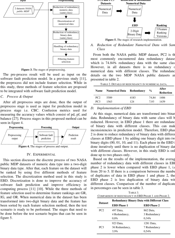
The preprocess stage consisted of five sub-processes i.e. reduction of redundant numerical data, discretization of numerical data, reduction of redundant binary data, handling the redundancy of binary data with different classes, and feature selection. Preprocess need to be done for making dataset suitable for learning model and to remove noise so that improve prediction result [26]. Preprocess stages of this research can be seen in figure 3.
Reduction of redundancy numeric data (same class) Discretization of numerical data Reduction of redundancy binary data (same class) Handling of redundancy binary data Filtering feature selection Preprocessing 2 datasets NASA public MDP Input
Figure 3. The stages of preprocessing.
The pre-process result will be used as input on the software fault prediction model. In a previous study [11], the preprocess did not include feature selection. While in this study, three methods of feature selection are proposed to be integrated with software fault prediction model. C. Process & Output
After all preprocess steps are done, then the output of preprocess stage is used as input for prediction model in process stage i.e. CBC. Confusion metrics used for measuring the accuracy values which consist of pd, pf, and balance [27]. Process stages in this proposed method can be seen in figure 4. Software fault prediction Processing Preprocessing output Preprocessing Prediction result Output
Figure 4. The stages of process and output. IV. EXPERIMENTAL
This section discusses the discrete process of two NASA public MDP datasets of numeric data type into a two-digit binary data type. After that, each feature on the dataset will be ranked by using five different methods of feature selection. The discretization method used in this study is EBD. Discretization is done to improve the accuracy of software fault prediction and improve efficiency in computing process [11] [10]. While the three methods of feature selection used to determine feature rankings are GR, IG, and OR. When numerical data in the dataset has been transformed into two-digit binary data and the feature has been sorted by each feature selection method, then the test scenario is ready to be performed. The stages that need to be done before the test scenario begins that can be seen in figure 5. Numerical Data PC2 and PC3 Datasets Numerical Data Reduction of Redundant Numerical Data 2-Digit Binary Data EBD 3 Feature Ranking Versions Ranking
Figure 5. The stages of research implementation.
A. Reduction of Redundant Numerical Data with Same Class
From both the NASA public MDP dataset, PC2 is the most commonly encountered data redundancy dataset, which is 74.84% redundancy data with the same class. However, in all datasets there is no redundancy of numerical data with different classes. The redundancy details on the two MDP NASA public datasets are presented in table 2.
TABLE 2.DETAILS OF REDUNDANCY IN NUMERICAL DATA.
Name Numerical Data Redundancy % After
Reduction PC2 PC3 5589 1563 4183 124 74,84 7,93 1406 1439 D. Implementation of EBD
At this stage, numerical data are transformed into binary data. Redundancy of binary data with same class will be reducted. However, in EBD phase 1 there are redundancy of binary data with different classes. This can make inconsistencies in prediction model. Therefore, EBD phase 2 is done to reduce redundancy of binary data with different classes at EBD phase 1 by adding one binary digit into two binary digits (00, 01, 10, and 11). Each phase in the EBD is done iteratively until there is no duplication of binary data with different classes. However, in this study EBD is only done up to two phases only.
Based on the results of the implementation, the average number of redundancy data with different classes in EBD phase 2 is lower when compared with EBD phase 1, i.e. from 20 to 5. If there is a comparison between the number of duplicates of data in EBD phase 1 and phase 2, then EBD phase 2 is less duplication of binary data with different classes. Comparison of the number of duplicates in percentages can be seen in table 3.
TABLE 3.
COMPARISON OF REDUNDANCY IN EBDPHASE 1 AND PHASE 2. Dataset Redundancy Binary Data with Different Class
EBD Phase 1 EBD Phase 2
PC2 497 Data, 4 Redundancy, 0,8% 862 Data, 3 Redundancy 0,34% PC3 923 Data, 36 Redundancy, 3,9% 1281 Data, 7 Redundancy 0,54%
E. Implementation of Feature Selection
After EBD two phases, the next stage that needs to be done before entering the testing phase is a feature selection. Output at this stage are three feature ranking GR, IG, and OR. In this phase, the PC2 and PC3 dataset will be sorted by all three methods of feature selection. There will be three versions of feature rank. The sequence of features is chosen iteratively to serve as input of CBC prediction modelConclusion
Some parameters of BMA and GOP, such as the weight and variance of BMA and the spatial parameters of GOP, should be estimated by iterative approach, for instance EM and L-BFGS respectively. For 30-day training period, the accuracy of BMA is not different than of the three members, while the former was more reliable, indicated by less CRPS. Furthermore, BMA manages to calibrate the forecast, indicated by the coverage closer to 50%. Lack of fit, though, is still owned by GOP since it has higher RMSE. From both method, BMA forecasts apparently have greater accuracy and precision.
V. RESULTS AND DISCUSSION
5-fold cross validation is used in this research for evaluating the experiment. Every test results on each fold is measured by confusion metrics. The pd and pf value will be used for measuring the average prediction values of CBC combination and determining the best feature selection method that the most improve CBC. The confusion matrix can be seen in table 4.
TABLE 4. CONFUSION MATRIX. Prediction Actual Faulty Non-faulty Faulty Non-faulty TP FN FP TN
For measuring pd and pf value can be seen in formula (1) and (2):
𝑝𝑝𝑝𝑝=(𝑇𝑇𝑇𝑇+𝐹𝐹𝐹𝐹𝑇𝑇𝑇𝑇 ) (1)
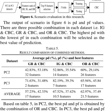
𝑝𝑝𝑝𝑝=(𝐹𝐹𝑇𝑇+𝑇𝑇𝐹𝐹𝐹𝐹𝑇𝑇 ) (2) Pd means successful value of prediction systems in predicting the software fault, while pf means misclassification value of prediction systems in determining unfaulty module as faulty module. The higher pd and the lowest pf are the best result. It means that system can predict the faulty module without giving the false alarm to the tester. In this research, CBC is combined with three methods of filtering feature selection (i.e. GR, IG, and OR). A number of features of dataset will be ranked by the feature selection method. Every selection feature method has different order of features rank. Then, the top N of features will be selected as CBC input. Illustration for this scenario can be seen in figure 6.
PC2 & PC3 datasets Features rank of GR, IG, and OR Top N features selection Training Features Rank
Input Feature Selection Cross validation Fault
Prediction
5 folds CBC
Testing Figure 6. Scenario evaluation in this research.
The output of scenario in figure 6 is pd and pf values. There are three possible combination in each dataset i.e. IG & CBC, GR & CBC, and OR & CBC. The highest pd with the lowest pf in each combination will be selected as the best value of prediction.
TABLE 5.
RESULT COMPARISON OF COMBINED METHODS. Dataset Average pd (%), pf (%) and best features
GR & CBC IG & CBC OR & CBC PC2 42.83%, 53.18% 32 features 52.86%, 35.54% 14 features 60%, 29,14% 26 features PC3 71.63%, 31.48% 2 features 82.19%, 39.3% 7 features 65.94%, 45.84 17 features AVERAGE 57.23%, 42.33% 17 features 67.52%, 37.42% 10.5 features 62.97%, 37.49 21.5 features Based on table 5, in PC2, the best pd and pf is obtained by the combination of OR and CBC. In PC3, the best pd and pf is obtained by the combination of IG and CBC. The combination of CBC and IG can generate the highest average pd value i.e. 67.52% pd and the lowest average pf value i.e. 37.42%.
When it compared to the CBC without filtering feature selection method, IG can increase pd 2.14% and reduce pf 12.53%. The end result can be seen in table 6.
TABLE 6.
COMPARISON OF THE BEST COMBINATION AND WITHOUT FEATURE SELECTION.
Dataset Average pd (%), pf (%) and best features IG & CBC No feature selection
PC2 52.86% pd, 35.54% pf, 14 features 49.28% pd, 55.11% pf, 36 features PC3 82.19% pd, 39.3% pf, 7 features 81.47% pd, 44.79% pf, 37 features AVERAGE 67.52% pd, 37.42% pf, 10.5 features 65.38% pd, 49.95% pf, 36.5 features VI. CONCLUSION
Based on the experiment and analysist, the combination of IG and CBC had the highest average value of prediction among of other feature selection method used in this research. It is proven that just a number of feature in software fault dataset which is relevant with the prediction class and filtering feature selection can improve CBC.
REFERENCES
[1] C. Catal, “Software fault prediction: A literature review and current trends,” Expert Syst. Appl., vol. 38, no. 4, pp. 4626–4636, Apr.
2011.
[2] P. Singh and S. Verma, “Software Fault Prediction Model for Embedded Systems: A Novel finding,” Int. J. Comput. Sci. Inf. Technol., vol. 5, no. 2, pp. 2348–2354, 2014.
[3] T. Hall, S. Beecham, D. Bowes, D. Gray, and S. Counsell, “A Systematic Literature Review on Fault Prediction Performance in Software Engineering,” IEEE Trans. Softw. Eng., vol. 38, no. 6, pp. 1276–1304, Nov. 2012.
[4] T. Menzies, J. Greenwald, and A. Frank, “Data Mining Static Code Attributes to Learn Defect Predictors,” IEEE Trans. Softw. Eng., vol. 33, no. 1, pp. 2–13, Jan. 2007.
[5] D. A. A. G. Singh, A. E. Fernando, and E. J. Leavline, “Experimental study on feature selection methods for software fault detection,” in 2016 International Conference on Circuit, Power and Computing Technologies (ICCPCT), 2016, pp. 1–6.
[6] T. Hall, S. Beecham, D. Bowes, D. Gray, and S. Counsell, “A Systematic Review of Fault Prediction Performance in Software Engineering,” IEEE Trans. Softw. Eng., vol. 38, no. 6, pp. 1276– 1304, 2012.
[7] R. Malhotra, “A systematic review of machine learning techniques for software fault prediction,” Appl. Soft Comput., vol. 27, pp. 504– 518, Feb. 2015.
[8] A. Kumar and D. Zhang, “Hand-Geometry Recognition Using Entropy-Based Discretization,” IEEE Trans. Inf. Forensics Secur., vol. 2, no. 2, pp. 181–187, Jun. 2007.
[9] P. Singh and S. Verma, “An Investigation of the Effect of Discretization on Defect Prediction Using Static Measures,” in 2009 International Conference on Advances in Computing, Control, and Telecommunication Technologies, 2009, pp. 837–839.
[10] P. Singh and O. P. Vyas, “Software Fault Prediction Model for Embedded Software : A Novel finding,” Int. J. Comput. Sci. Inf. Technol., vol. 5, no. 2, pp. 2348–2354, 2014.
[11] P. Singh and S. Verma, “An Efficient Software Fault Prediction Model using Cluster based Classification,” Int. J. Appl. Inf. Syst., vol. 7, no. 3, pp. 35–41, 2014.
[12] D. A. Antony, G. Singh, A. E. Fernando, and E. J. Leavline, “Software Fault Detection using Honey Bee Optimization,” Int. J. Appl. Inf. Syst., vol. 11, no. 1, pp. 1–9, 2016.
[13] M. S. Akbar, “Prediksi Cacat Perangkat Lunak Dengan Optimasi Naive Bayes Menggunakan Pemilihan Fitur Gain Ratio,” Institut Teknologi Sepuluh Nopember, 2017.
[14] J. Novakovic, “The Impact of Feature Selection on the Accuracy of Naive Bayes Classifier,” 18th Telecommun. forum TELFOR, vol. 2, pp. 1113–1116, 2010.
[15] E. Erturk and E. A. Sezer, “A comparison of some soft computing
methods for software fault prediction,” Expert Syst. Appl., vol. 42, no. 4, pp. 1872–1879, Mar. 2015.
[16] S. Lessmann, B. Baesens, C. Mues, and S. Pietsch, “Benchmarking Classification Models for Software Defect Prediction: A Proposed Framework and Novel Findings,” IEEE Trans. Softw. Eng., vol. 34, no. 4, pp. 485–496, Jul. 2008.
[17] L. Ladha and T. Deepa, “Feature Selection Methods and Algotithms,” Int. J. Comput. Sci. Eng., vol. 3, no. 5, pp. 1787–1797, 2011.
[18] A. Gowda Karegowda, A. S. Manjunath, and M. A. Jayaram, “Comparative Study of Attribute Selection using Gain Ratio and Correlation Based Feature Selection,” Int. J. Inf. Technol. Knowl. Manag., vol. 2, no. 2, pp. 271–277, 2010.
[19] Feihu Yang, Weiqing Cheng, Renfu Dou, and Ningning Zhou, “An improved feature selection approach based on ReliefF and Mutual Information,” in International Conference on Information Science and Technology, 2011, pp. 246–250.
[20] G. Abaei and A. Selamat, “A survey on software fault detection based on different prediction approaches,” Vietnam J. Comput. Sci., vol. 1, no. 2, pp. 79–95, 2014.
[21] G. Chandrashekar and F. Sahin, “A survey on feature selection methods,” Comput. Electr. Eng., vol. 40, no. 1, pp. 16–28, Jan. 2014.
[22] P. Singh, N. R. Pal, S. Verma, and O. P. Vyas, “Fuzzy Rule-Based Approach for Software Fault Prediction,” IEEE Trans. Syst. Man, Cybern. Syst., pp. 1–12, 2016.
[23] C. Akalya Devi, K. E. Kannammal, and B. Surendiran, “A Hybrid Feature Selection Model for Software Fault Prediction,” Int. J. Comput. Sci. Appl., vol. 2, no. 2, pp. 25–35, 2012.
[24] K. Gao, T. M. Khoshgoftaar, H. Wang, and N. Seliya, “Choosing software metrics for defect prediction: an investigation on feature selection techniques,” Softw. - Pract. Exp., vol. 39, no. 7, pp. 701– 736, 2011.
[25] D. H. Murti, N. Suciati, and D. J. Nanjaya, “Clustering data non-numerik dengan pendekatan algoritma k-means dan hamming distance studi kasus biro jodoh,” J. Ilm. Teknol. Inf., vol. 4, pp. 46– 53, 2005.
[26] D. Gray, D. Bowes, N. Davey, Yi Sun, and B. Christianson, “The misuse of the NASA Metrics Data Program data sets for automated software defect prediction,” in 15th Annual Conference on Evaluation & Assessment in Software Engineering (EASE 2011), 2011, pp. 96–103.
[27] C. Catal, “Performance Evaluation Metrics for Software Fault Prediction Studies,” Acta Polytech. Hungarica, vol. 9, no. 4, pp. 193–206, 2012.