University of South Florida University of South Florida
Scholar Commons
Scholar Commons
Graduate Theses and Dissertations Graduate School
July 2016
Efficient Algorithms and Applications in Topological Data Analysis
Efficient Algorithms and Applications in Topological Data Analysis
Junyi TuUniversity of South Florida, [email protected]
Follow this and additional works at: https://scholarcommons.usf.edu/etd
Part of the Computer Sciences Commons, and the Mathematics Commons Scholar Commons Citation
Scholar Commons Citation
Tu, Junyi, "Efficient Algorithms and Applications in Topological Data Analysis" (2016). Graduate Theses and Dissertations.
https://scholarcommons.usf.edu/etd/8083
This Dissertation is brought to you for free and open access by the Graduate School at Scholar Commons. It has been accepted for inclusion in Graduate Theses and Dissertations by an authorized administrator of Scholar
Efficient Algorithms and Applications in Topological Data Analysis
by
Junyi Tu
A dissertation submitted in partial fulfillment of the requirements for the degree of
Doctor of Philosophy
Department of Computer Science and Engineering College of Engineering
University of South Florida
Major Professor: Paul Rosen, Ph.D. Les Piegl, Ph.D. Yicheng Tu, Ph.D. Zhuo Lu, Ph.D. Dmytro Savchuk, Ph.D. Date of Approval: November 7, 2019
Keywords: Reeb Graphs, Contour Trees, Parallel Computing, Persistent Pairing, Image Enhancement
Dedication
Acknowledgments
I am deeply indebted to my adviser, Dr. Paul Rosen, without whom I would not have a chance to earn a Ph.D in Computer Science and Engineering. Especially at the same time I am starting a family in a foreign country. Without the support from my adviser, I can not survive this adventure. The training in CSE is very different from my previous training in mathematics, it really broadens my horizon to another dimension in computers invented less than one hundred years ago. I would also like to extend my deepest gratitude to my committee members for their encouragement and advice: Dr. Yicheng Tu, Dr. Les Piegl, Dr. Zhuo Lu and Dr. Dmytro Savchuk. Special thanks go to my defense chairperson, Dr. Alon Friedman, who also provided feedback to improve this dissertation.
I would like to thank several other faculty members from whom I have learned a lot in programming languages, machine learning and computer security. Those professors include Dr. Dmitry B. Goldgof, Dr. Jarred Ligatti, Dr. Yu Sun, Dr. Hao Zheng, Dr. Larry Hall and many others. I owe a lot to Dr. Yuncheng You for his encouragement and support. I am grateful to my internship hosts, Dr. Schanen Michel and Dr. Kibaek Kim in Argonne National Lab, they gave me a rare chance to see the research involving both mathematics and computer science. My classmates and friends also help me a lot, I especially want to thank Bingxiong Lin, Jie Zhang, Lei Wu, Xiaofan Xu, Yuqi Huang, Zhaolin Jiang, Nan Zhao, Jun Cheng, Yongqiang Huang, Ran Rui, Renhao Liu, Jiayi Wang, Xiaoshan Wang, Mark Hoel, ATM Golam Bari, Cagri Cetin, Jean-Baptiste Subils, Chengcheng Mou and many others. I must also thank my great labmates: Zachariah J. Beasley, Tanmay Kotha, Ghulam Jilani Quadri, and Zhila Nouri. Last but not least, I want to thank the staff of the CSE main office, especially Laura and Gabriela, for their help and the entire department for their warmth and
Table of Contents List of Tables iv List of Figures v Abstract viii Chapter 1: Introduction 1 1.1 Motivation 1 1.2 Contribution 4 Chapter 2: Background 7 2.1 Critical Points 7 2.2 Contour Tree 7 2.3 Reeb Graph 10 2.4 Mapper 11
2.5 Critical Point Pairing 13
2.5.1 Persistent Homology and Persistence Diagram 13
Chapter 3: Parallel Computation of Merge Tree 17
3.1 Introduction 17
3.2 Conventional Merge Tree Construction 19
3.3 Parallel Merge Tree Construction 21
3.3.1 Phase 1: Coloring 21
3.3.2 Phase 2: Potential Critical Point Extraction 22
3.3.3 Phase 3: Saddle Sorting 23
3.3.4 Phase 4: Subtree Building and Merge Propagation 24
3.4 Extension to 3D and Higher Dimensions 24
3.5 OpenCL Implementation 25
3.6 Experiments 25
3.6.1 Random Field Tests 25
3.6.2 Contour Trees in Radio Astronomy Data 28
Chapter 4: Critical Point Pairing in Reeb Graphs 31
4.1 Introduction 31
4.2 Reeb Graph 33
4.2.1 Persistence Diagram of Reeb Graph 35
4.2.1.1 Branching Features of Reeb Graph 35
4.2.1.2 Cycle Features of Reeb Graph 36
4.3 Related Work 36
4.4 Conditioning the Graph 37
4.5 Multipass Approach 39
4.5.1 Non-Essential Fork Pairing 40
4.5.2 Essential Fork Pairing 41
4.6 Single-Pass Algorithm: Propagate and Pair 43
4.6.1 Basic Propagate and Pair 44
4.6.2 Virtual Edges for Propagate and Pair 45
4.7 Evaluation 49
4.8 Conclusions 55
Chapter 5: Contrast and Brightness Enhancement of Color Image 57
5.1 Introduction 57
5.1.1 Computing the Contour Tree 60
5.2 Capturing the Topology of an Image 62
5.2.1 Feature Subtree Extraction 62
5.2.2 The Contour Tree of Color Images 62
5.3 Image Processing via Contour Trees 62
5.3.1 Visualizing the Contour Tree 63
5.3.2 Subtree Selection as Image Segmentation 65
5.3.3 Subtree Modification as Image Editing 66
5.4 Examples 68
5.5 Conclusions 73
Chapter 6: Application of Mapper in Point Cloud-based 3D Printed Objects 77
6.1 Introduction 77
6.2 Mapper and Persistent Homology 77
6.2.1 Mapper 78
6.2.2 Persistent Homology 80
6.2.3 Link Between Mapper and Persistent Homology 81
6.3 The Topology of 3D Printing 82
6.3.1 Visualization 82
6.4 Results 83
6.4.1 Original Model 85
6.4.2 Error Corrected Model 87
6.4.3 Runtime Performance 87
Chapter 7: Conclusion and Future Work 90
7.1 Summary 90
7.2 Vision 90
References 92
List of Tables
List of Figures
Figure 1.1 Topological Data Analysis Pipeline. 3
Figure 2.1 Critical points of a scalar function. 7
Figure 2.2 Contour tree calculation on a scalar field. 9
Figure 2.3 Reeb graph on a manifold with a function. 10
Figure 2.4 Mapper on a point cloud model. 12
Figure 2.5 Example of persistence diagram. 16
Figure 3.1 Three existing strategies used to parallelize merge tree construction. 19 Figure 3.2 Example of 2D scalar field used to describe our parallelization
of merge tree construction. 19
Figure 3.3 Illustration of conventional merge tree construction. 20
Figure 3.4 Illustration of the four phases of parallel merge tree construction. 22
Figure 3.5 Example of noisy scalar fields used for performance testing. 26
Figure 3.6 Charts of the performance of our parallel merge tree algorithm
on random fields. 27
Figure 3.7 Visualization of Radio Astronomy Data. 29
Figure 3.8 Performance on Radio Astronomy Data. 30
Figure 4.1 Reeb graph and persistence diagram. 33
Figure 4.2 Cases for Reeb graph conditioning. 37
Figure 4.3 Example of multipass critical point paring. 39
Figure 4.4 Illustration of the four case for non-essential fork pairing in the
Figure 4.5 Illustration of non-essential fork pairing in the multipass algorithm. 42
Figure 4.6 The join tree-based essential fork pairing for up-fork D. 43
Figure 4.7 Essential fork pairing in the multipass algorithm for the example
Reeb graph from Figure 4.3. 44
Figure 4.8 Propagate and Pair algorithm on the example Reeb graph from
Figure 4.3. 46
Figure 4.9 Continuation of Figure 4.8. 47
Figure 4.10 An example case of where the basic propagate and pair algorithm fails. 47
Figure 4.11 An example requiring virtual edge merging. 48
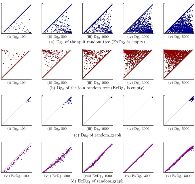
Figure 4.12 Persistence diagrams for random trees and random graphs. 51
Figure 4.13 Meshes and Reeb graphs used in evaluation. 52
Figure 4.14 Continuation of Figure 4.13. 53
Figure 4.15 Performance on random split/join trees and graphs. 54
Figure 4.16 Persistence diagram of SCIVIS contest data. 55
Figure 4.17 Performance results when cutting cycles in the random graph 5000. 56
Figure 5.1 Contour tree on a terrain. 58
Figure 5.2 Contour tree and its decomposition. 59
Figure 5.3 Interfaces used for selecting topological features. 64
Figure 5.4 Example of segmentation based on persistence diagram. 65
Figure 5.5 Four functions based on subtree editing. 67
Figure 5.6 Illustration of four functions on scalar field 69
Figure 5.7 Evaluation on Florala dataset. 71
Figure 5.8 Evaluation on Brain dataset. 72
Figure 5.9 Evaluation on Lenna Grayscale dataset 73
Figure 5.10 Evaluation on Notre Dame dataset. 74
Figure 5.12 Evaluation on Swan dataset. 76
Figure 6.1 Multilayers filled/Empty space topology. 78
Figure 6.2 Example of Mapper on a mesh. 79
Figure 6.3 Example of Mapper on the empty space of a mesh. 80
Figure 6.4 Example of persistent homology 81
Figure 6.5 Our software with the Stanford Dragon dataset. 83
Figure 6.6 Results of Dragon dataset. 84
Figure 6.7 Error Corrected Results of Dragon dataset. 86
Abstract
Topological Data Analysis (TDA) is a new and fast growing research field developed over last two decades. TDA finds many applications in computer vision, computer graphics, scientific visualization, molecular biology, and material science, to name a few. In this dissertation, we make algorithmic and application contributions to three data structures in TDA: contour trees, Reeb graphs, and Mapper. From the algorithmic perspective, we design a parallel algorithm for contour tree construction and implement it in OpenCL. We also design and implement critical point pairing algorithms to compute persistence diagrams directly from contour trees, Reeb graphs, and Mapper. In terms of applications, we apply TDA in the design and implementation of an image enhancement application using contour trees. Lastly, we introduce an application of Mapper and persistent homology in model quality assessment for 3D printing.
Chapter 1: Introduction
1.1 Motivation
Geometric shapes are ubiquitous in many datasets from computer graphics, computer aided design, computer vision, and data visualization. These research fields utilize count-less problems in computational geometry, such as convex hull, Voronoi diagrams, Delaunay triangulation, polygon partitioning, and geometric searching. Many efficient and effective algorithms to solve these problems are presented in the classic textbook by Franco Preparata and Michael Shamos [61].
Topology studies the properties of a geometric object that are preserved under continuous deformation, such as stretching, twisting, and bending, but not tearing. One common ex-ample of continuous deformation is transforming a coffee mug into a donut. Each is a single component with one hole, i.e., the mug handle and donut hole. In other words, topologists do not see a difference between the shape of a coffee mug and a donut. An early precuror to modern topology was the well-known “Seven Bridges of K¨onigsbergan”, which Leonhard Eu-ler (1707–1783) proved had no solution and inspired the polyhedron formulaV −E+F = 2, where V, E, and F denoting the number of vertices, edges, and faces of the polyhedron, respectively. Topology can also reveal the intrinsic secrets of exotic matter—the 2016 Nobel Prize in Physics was awarded to David J. Thouless, F. Duncan M. Haldane, and J. Michael Kosterlitz, “for theoretical discoveries of topological phase transitions and topological phases of matter” [37].
Unfortunately, combining topological invariants with geometry to solve real world prob-lems is nontrivial. Approximately two decades ago Topological Data Analysis (TDA) began to bridge this gap, most notably with the work on persistent homology by Herbert Edels-brunner [35], Afra Zomorodian [90], and Gunnar Carlsson [14]. The classic workflow of TDA is as follows: the input of TDA pipeline is a point cloud dataset; then, a filtration, a nested sequence of complexes, such as the alpha complex, is built on the point cloud; next, the homology of each complex in the filtration is used to calculate the persistence module; lastly, the matrix reduction algorithm produces thepersistence diagram, which characterizes the topological features by defining a scale parameter that tracks the birth and death, i.e., appearance and disappearance, of features continuously over all spatial resolutions. The persistence diagram is often visualized as a scatterplot of the same name, i.e., a persistence diagram, which indexes topological features by their “life-time” in the filtration.
Visualization has been used to analyze and understand data for decades [22, 81], and TDA combines both data analysis and visualization seamlessly. Topology-based techniques for analyzing data are becoming increasingly popular due in large part to their robustness and their applicability to a wide variety of datasets and scientific domains, from cancer research [54] to sports analytics [4], to collaboration [7, 19] and brain networks [20, 25], among others [15, 46, 47, 51, 77, 53]. Many open-source libraries and software packages have been developed for the computation of persistent homology, such as Dionysus [48], JavaPlex [1], PHAT (Persistent Homology Algorithm Toolkit), and DIPHA (Distributed Persistent Homology Algorithm) [9], among many others. [56] provides a detailed analysis of software packages and tutorial for the computation of persistent homology on point cloud datasets.
Another branch of TDA uses other data structures, including contour trees [12], Reeb graphs [63], and Mapper [70], to compute persistence and persistence-like features under special conditions or on other types of data, e.g., manifolds [13]. These tools are useful for
computing persistence on data that do not easily fit in the persistent homology pipeline, such as a function applied to a 2-manifold, i.e., the Buddha mesh, or a simple domain, i.e., the grayscale image, in Figure 1.1.
Persistence
Diagram
Image
3D Mesh
Reeb Graph
Contour Tree
Mapper
Point Cloud
Point Cloud
Persistent Homology
Image Enhancement Data Visualization Topological Denoising 3D printing Quality inferring
Figure 1.1. Topological Data Analysis Pipeline. The Topological Data Analysis pipeline we discuss focuses on three types of data, point clouds, 3D meshes, and images. Their topological structure can be extracted using four data structures, all of which can be visualized as persistence diagrams. On the right are four applications of the persistence diagram studied in this dissertation.
The Reeb graph [63] was first introduced in the mid-19th century. A more detailed introduction to the Reeb graph is included in the Background chapter, but in short, Reeb
graph encodes the evolution of the connectivity of the level sets induced by a scalar function defined on a data domain by sweeping from negative infinity to positive infinity and tracking the birth and death of the connected components of the level sets. A non-looping Reeb graph is called the contour tree [12], and an approximation for the Reeb graph can be computed using Mapper [70].
One challenge with using Reeb graphs to directly analyze data is that the graphs they produce are frequently too large or complex to directly visualize, therefore requiring further abstraction. The notion of persistence can be applied to any act of birth that is paired with an act of death. Since the Reeb graph encodes the birth and the death of the connected components of the level sets of a scalar function, the notion of persistence can be applied to pair the critical points in the Reeb graph [2].
Reeb graphs, contour trees, and Mapper have found many applications in computer graphics, computer vision, and scientific visualization. They have been successfully used in feature detection [73], data reduction and simplification [17, 68], image processing [45], shape understanding [5], visualization of isosurfaces [6], analysis and visualization tool of radio astronomy data [66], etc. One widely used tool for this type of computation is the Topology ToolKit (TTK) [75], which primarily computes contour trees and Reeb graphs on triangulated mesh data in 2D and 3D. These algorithms are the main focus of this dissertation (see Figure 1.1).
1.2 Contribution
When broadly considering TDA, we address two main areas of need. The first is in efficient and parallel algorithms for computing TDA data structures, particularly for large data. TDA calculations tend to be either expensive to compute, e.g., persistent homology is O(n3), or extremely difficult to parallelize, e.g., contour trees require a partial ordering
of TDA in domain applications. In these domains it may be nontrivial to map the domain problem to a TDA data structure, therefore requiring redesigning the TDA data structure.
In this dissertation, we address both the algorithmic and application challenges of TDA using three data structures: contour trees, Reeb graphs, and Mapper.
• First, we design and implement an efficient approach to parallel computation of a merge tree on a graphical processing unit (GPU). The merge tree represents an essential component and major bottleneck to building a contour tree or Reeb graph.
• Second, we design and implement two algorithms for efficient computation of the crit-ical point pairing in Reeb graphs, contour trees, and Mapper.
• Third, we adapt the contour tree to the application of color image enhancement. In this work we generalize topology-based denoising to introduce new topology-based trans-fer functions, including contrast enhancement, brightness enhancement, and gamma correction, that can be applied to contour trees to interactively enhance color images. • Lastly, we study an application of TDA in assessing the quality of point cloud-based 3D printed objects. In particular, we present an approach that uses a hybrid of Mapper and persistent homology to identify anomalies in point cloud models that may produce printer errors.
In summary, this dissertation demonstrates that the algorithms of TDA can be efficiently implemented and used in a wide variety of applications to solve real world problems. The dissertation is organized as follows. In Chapter 3, we present the parallel computation of merge tree. Chapter 4 is devoted to the algorithms of critical point pairing in Reeb graphs, one multi-pass and one single-pass algorithm. In Chapter 5, we show the application of contour tree and persistence diagrams in color images enhancement. Chapter 6 presents an application of Mapper and persistent homology in assessing the quality of models for point
cloud-based 3D printed objects. Finally, we conclude our work and present future directions in Chapter 7.
Chapter 2: Background
2.1 Critical Points
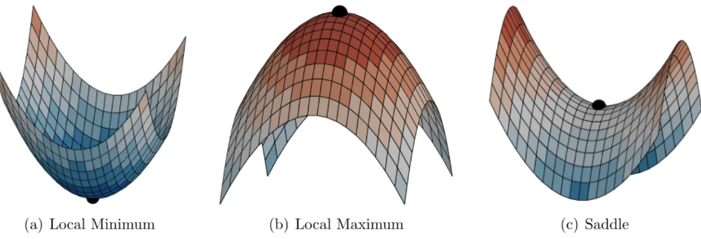
The topological data structures that this dissertation focuses on, specifically contour trees, Reeb graphs, and Mapper, are all concerned with capturing three geometric properties of data, local minima, local maxima, and saddle points (Figure 2.1). These being the three cases when the local function tangent is 0. These critical points are useful for tasks, such as hierarchical visualization [6, 17], segmentation [28, 72], or tracing structures [83] in scalar field data.
(a) Local Minimum (b) Local Maximum (c) Saddle
Figure 2.1. Critical points of a scalar function. Functions representing critical points: (a) lo-cal minimum, (b) lolo-cal maximum, and (c) a saddle point.
2.2 Contour Tree
Contour tree was first introduced by Boyell and Ruston [12] in 1963, who named it the “enclosure tree” of contour lines for the height of terrain. After an efficient serial algorithm
was introduced by Carr et al. [16], the contour tree became a popular tool in scientific visualization due to its ability to capture the topological structure of scalar fields. Contour trees have been used in many applications, such as isoline extraction in geometric data by van Krevald et al. [83], which provided the first formal algorithm, fast extraction of isosurfaces and interactive data exploration [58], volume rendering [85], uncertain terrains [88], and noise removal that does not negatively impact important features in the data [68].
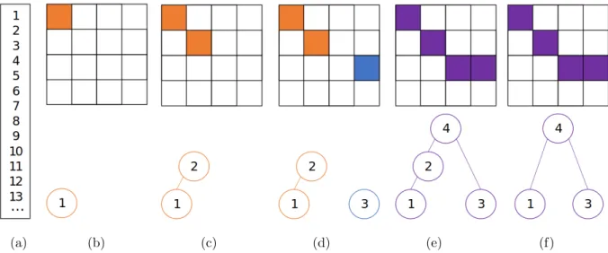
The contour tree (see Figure 2.2(c)) is obtained by contracting the connected components of the levelsets (i.e., the isocontours) of a function defined on a simple domain (i.e., a domain without any non-trivial homology) to a point and tracking the evolution of those levelsets. The construction of the contour tree can be decomposed into two parts, the join tree (see Figure 2.2(e)) and split tree (see Figure 2.2(g)), both of which are obtained using a merge tree that sweeps the function from bottom-to-top and top-to-bottom, respectively. As the merge tree sweeps the function, it tracks connected components in what are known as augmented versions of the trees. The final trees are found by removing non-critical points (those with one down edge and one up edge).
Figure 2.2 shows an example of contour tree construction. In Figure 2.2(a), a 4-by-4 scalar field is represented by color from black (lower value) and white (higher value). To construct the contour tree, the augmented join tree (see Figure 2.2(d)) and augmented split tree (see Figure 2.2(f)) are found and combined into an augmented contour tree (see Figure 2.2(b)). When non-critical points are removed from those trees, the join tree (see Figure 2.2(e)), split tree (see Figure 2.2(g)) and contour tree (see Figure 2.2(c)) are found.
The time complexity of Carr et al.’s algorithm is O(nlogn), primarily coming from a global sorting of points required to compute the augmented join and split trees. Furthermore, the algorithm requires a complete global ordering of data to guarantee the correct output. However, it can be shown, as we do in Chapter 3, that partial ordering is sufficient for most aspects of the algorithm, enabling the opportunity for parallelism.
a
b
c
d
e
f
g
h
i
j
k
l
m
n
o
p
(a) Scalar Field
o
j
a
h
i
f
g
e
c
d
b
n
m
l
k
p
o
j
a
h
i
f
g
e
c
d
b
n
m
l
k
p
o
h
i
g
e
c
d
n
m
l
k
p
j
a
f
b
(b) Augmented Contour Tree (c) Contour Tree
o
j
a
h
i
f
g
e
c
d
b
n
m
l
k
p
o
j
a
h
i
f
g
e
c
d
b
n
m
l
k
p
o
h
i
g
e
c
d
n
m
l
k
p
j
a
f
b
(d) Augmented Join Tree (e) Join Tree
o
j
a
h
i
f
g
e
c
d
b
n
m
l
k
p
o
j
a
h
i
f
g
e
c
d
b
n
m
l
k
p
o
h
i
g
e
c
d
n
m
l
k
p
j
a
f
b
(f) Augmented Split Tree (g) Split Tree
Figure 2.2. Contour tree calculation on a scalar field. The (a) scalar field has its (b) aug-mented contour tree calculated by combining the (d) augaug-mented join tree and (f) augaug-mented split tree. The critical points of the augmented trees are used to generate the (c) contour tree, (e) join tree, and (g) split tree.
2.3 Reeb Graph
Reeb graph is named after French mathematician Georges Reeb (1920–1993), who pro-posed the graph as a tool in Morse theory around 1946 [63]. The Reeb graph is obtained similarly to the contour tree by contracting the connected components of the levelsets of a function. In this case, the function is defined on a manifold with non-trivial homology (e.g., holes/tunnels). In fact, the contour tree is an acyclic Reeb graph. It provides a skeletonized summarization of both geometrical shape and its relationship with the scalar function. Hence, it is an instrumental data structure to encode the topological properties of geometric objects. Figure 2.3 shows an example Reeb graph captured from a manifold with a scalar function defined on it.
G E D P I F L J K M H N O A B C A B G E D P C I F L J K M H N O
(a) Manifold with a scalar function
G E D P I F L J K M H N O A B C A B G E D P C I F L J K M H N O (b) Reeb graph
Figure 2.3. Reeb graph on a manifold with a function. The (a) manifold with a scalar function is processed into (b) a Reeb graph that encodes both the geometric shape and its relationship to the scalar function.
Reeb graphs and contour trees have found numerous applications in graphics and visu-alization including data skeletonization [38], locus cut [26], data abstraction [52], retrieving topological information from point data, such as homology group computation [27, 21], vol-ume rendering [86], and terrain applications [10, 40].
The first algorithm to compute Reeb graph on a triangulated surface was presented by Shinagawa and Kunii [69], with time complexity O(n2), where n is the number of triangles in the mesh. The efficient computation of Reeb graphs has been an active research topic for last two decades. Cole-McLaughlin et al. [24] improved the performance to O(nlogn). Pascucci et al. [60] presented an online method to compute Reeb graphs. Harvey et al. [42] deployed a randomized algorithm to compute Reeb graph on arbitrary simplicial complexes
K in expected timeO(mlogn), wheremis the size of 2-skeleton ofK (i.e., the total number of vertices, edges, and triangles), and n is the number of vertices. For the application of Reeb graphs, Hilaga et al. [43] provide a Multi-resolution Reeb Graph (MRG) representation of triangle meshes which is independent of rotation in topology matching. By reducing the Reeb graph to contour tree via loop surgery, Tierny et al. [76] presented an algorithm to compute Reeb graph on a volumetric mesh inR3. In a similar vein, the work by Doraiswamy
and Natarajan [31] utilizes the union of contour trees to compute the Reeb graph. Other Reeb graph algorithms can be found in [29, 30, 57].
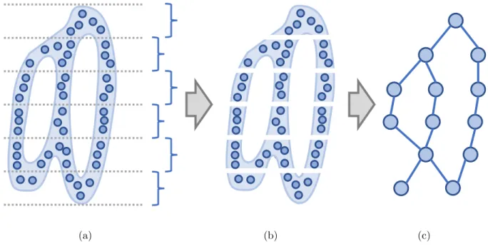
2.4 Mapper
The Mapper is a relatively new concept introduced by Gurjeet Singh, Facundo M´emoli, and Gunnar Carlsson in 2007 [70]. It is an efficient topological method to reduce high dimensional datasets into a graph by applying a topological lens to data that captures specific limited topological information of the high dimensional datasets at a specified resolution.
Mapper construction (see Figure 2.4) starts with a dataset X and a topological lens, real valued function f : X −→ R, on the data. We choose the open covering of the range
of f, with overlapping of the neighboring covers. Then, the pre-image of each open set in the covering is an open cover of the dataset X. The output graph vertices are created from connected components, found via clustering, within each topological cover (i.e., open set). In other words, the connected components of one open set are “collapsed” into output graph vertices. The output graph edges are added between components that contain the same points fromX. The resulting graph can describe the overall topology of the connected components of the dataset under the provided topological lens.
(a) (b) (c)
Figure 2.4. Mapper on a point cloud model. Using Mapper to construct a topological skele-ton, first the (a) point cloud-based model is (b) sliced. (c) Connected components are collapsed to vertices and edges added for components that touch.
The first algorithm for Mapper construction comes in its original paper [70]. [41] provided a provably correct algorithm of parallel computation of Mapper and reported performance experiments on the efficiency of distributed Mapper. Mapper is also one of the main algo-rithms underlying the tools sold by Ayasdi AI LLC [3], though their implementation is not public.
Mapper can be observed to be an approximation of a Reeb graph. Both the Reeb graph, including the contour tree, and Mapper essentially provide a topological description of the dataset, but their representations of the topological information are different in the following sense. The nodes of the Reeb graph represent the critical points of the underlying scalar field, and the edges of Reeb graph represent the collapsed connected components in the domain where there is no topological change. On the other hand, the nodes in Mapper represent one cluster of data points and the edges are formed because of the common data points in two pre-images from neighboring projection intervals.
2.5 Critical Point Pairing
Persistent homology [32] is the main concept in TDA. Within the framework of TDA, the individual topological features in the Reeb graph, such as cycles, can be ordered according to their birth time and death time (i.e., the function value where the feature appears and disappears). The birth and death times of topological features (equivalently, the paired critical points) can be seen as a signature for Reeb graph [13].
Here we provide a brief and limited introduction to persistent homology, since the neces-sary concepts from algebraic topology are quite involved. Fortunately, we have an intuitive explanation of topological persistence in contour trees and Reeb graphs in Chapter 4, when we describe an effective algorithm to compute the critical point pairs.
2.5.1 Persistent Homology and Persistence Diagram
The concept of persistent homology was developed by Edelsbrunner et al. [35]. Here we present the theoretical setting for the computation of the persistence diagram associated with a scalar function defined on a triangulated topological space. We then show how this is related to the critical point pairing on Reeb graphs in Chapter 4. We start by presenting a concise description of persistent homology of a finitely triangulable topological space with a
continuous function defined on it. For the treatment of persistent homology of general point cloud dataset, the reader is referred to [33, 89].
Let X be a triangulable topological space, and let f :X →IR be a continuous function defined on it. Let r ∈ IR. We denote the sublevel set of f by X≤r ={x ∈ X | f(x) ≤ r}.
Similarly, we denote the superlevel set of f by X≥r = {x ∈ X | f(x) ≥ r}. Let Hp(X)
is the p-th homology group of X. We consider homology with coefficients in a finite field, so Hp(X) is a vector space. Let {r1, ..., rn} be a finite strictly increasing sequence of real
numbers. Consider the sequence of vector spaces:
0 = Hp(X0)→Hp(X1)→ · · · →Hp(Xn) =Hp(X), (2.1)
where Xi = X≤ri and each homomorphism g i+1
i : Hp(Xi) → Hp(Xi+1) on the homology
groups is induced by the inclusionXi ,→Xi+1. We can definegji :Hp(Xi)→Hp(Xj) for any
i≤j by composition. We say that a class α is born at ri if :
α ∈Hp(Xi) but α /∈imgii−1.
A class α born at ri dies at rj if:
gij(α)∈imgji−1 but gij−1(α)∈/imgij−1−1.
In this case, the function value pair (ri, rj) is called a persistence pair, and the difference
rj−riis thepersistence of the pair. When no confusion occurs, the pairing of function values
induces the critical point pairing in Reeb graphs. In other words, when we have a one to one correspondence between critical points and function values, we just represent persistence pairs using the critical points.
These birth and death events are captured by the notion of persistent homology. Specifi-cally, thep-th ordinary persistence diagram of f is a scatterplot, including multi-set of pairs (b, d), where b and d are corresponding to the birth function value and death function value of some p-dimensional homology class, respectively. We denote thep-th ordinary persistence diagram of f by Dgp(f). In general, the homology group Hp(X) is non-trivial. We call a
non-trivial homology class in Hp(X) an essential homology class, they will never die during
the sequence in Equation 2.1. These non-trivial homology classes are express the cyclic fea-tures in Reeb graph. By augmenting an array of relative homology groups to Equation 2.1, we have the following sequence:
0 =Hp(X0)→ · · · →Hp(Xn) =Hp(X) =
Hp(X, X≥rn)→Hp(X, X≥rn−1)→ · · · →Hp(X, X≥r0) = 0. (2.2)
Since the final vector space Hp(X, X≥r0) = 0, every essential homology class eventually dies
in some relative homology groupHp(X, X≥rj). In other words, each essential homology class in a homology group Hp(Xi) will die at some relative homology group Hp(X, X≥rj), so we have a pair (ri, rj), with ri ≥ rj by the property of relative homology group. We call the
scatterplot of multi-set of these pairs the pth extended persistence diagram. We denote it by ExDgp(f). In other word, for each point (b, d) in ExDgp(f), there is an essential homology class in Hp(X), which is born in Hp(X≤b) and dies at Hp(X, X≥d). Observe that for the
extended persistence diagram the birth value b is greater than or equal to death value d. To compute these pairs, branch decomposition was first used to provide a multi-scale view of critical points in contour trees [59]. This provides the framework for pairing non-essential critical points in a Reeb graph. The first known description of pairing critical points of a Morse function on a 2-manifold, including essential critical points, is given in [2]. However,
the description is high level with no specific algorithm provided. A similar description of persistence pairing algorithm is also seen in [8].
After the critical points are paired, they can be visualized using a persistence diagram (see Figure 2.5). These scatterplot charts show each pair as a single point, parameterized by birth on the horizontal axis and death on the vertical axis. In addition to serving as a signature for the topology of the input data, a major advantage of persistence diagrams is simplicity and scalability—a large Reeb graph can be reduced to a much easier to interpret scatterplot. P O N M L K J I H G F E D C B A A B G E C P N O K H A B C D E F G H I J K L M N O P B,C E,G O,N H,K
A,P Pd0of sublevel sets
Pd 0of su pe rle ve l s ets
Figure 2.5. Example of persistence diagram. The persistence diagram, Dg0(f), for the Reeb graph in Figure 2.3 shows topological feature as points, parameterized by birth horizontally and death vertically.
Pairing of critical points of a scalar function has found multiple applications including segmentation of deformable shapes [71], hierarchical shape segmentation [64], description of protein shape [87], automatic extraction of surface structures [84], and 3D shape description and matching [11].
Chapter 3: Parallel Computation of Merge Tree
This chapter1 introduces the data structure of merge tree and its parallel computation.
3.1 Introduction
Scalar fields are used to describe a variety of details from photographs, to laser scans, to x-ray, CT, or MRI scans. These scalar fields are invaluable for a variety of tasks, such as fatigue detection in machine parts, medical diagnosis, etc. However, analyzing scalar fields can be quite challenging due to their size, complexity, and the need to understand both local details and global context.
The merge tree is the key data structure used in the computation of the join tree, split tree, and contour tree [16]. However, computing these trees is expensive, and their incre-mental construction makes parallel computation nontrivial.
In its naive implementation, the algorithm to compute merge trees seems efficient. No matter the dimension of the data, it has anO(nlogn) sort phase and anO(n+k) computation phase, wherenis the number of elements in the scalar field andkis the aggregate cost of the find operation of a disjoint-set data structure. However, this algorithm has three practical challenges. First, as the dimension of the field is doubled, the number of elements grows quadratically in 2D fields and cubically in 3D fields. Secondly, although asymptotically small, the actual compute time per element in the computation phase is very high. Third, the
1Part of this chapter was published in Computer-Aided Design and Applications (2018) [67]. Permission
computation phase requires partially ordered incremental construction, making it a challenge to parallelize.
While the global sort can be avoided [62], the algorithm is still difficult to parallelize. Three strategies have been proposed to parallelize merge tree calculations: pruning [18], spatial-domain parallelization [49, 50], and value-domain parallelization [39]. Pruning (see Figure 3.1(a)) works by eliminating elements from the computation, which are predetermined not to be a local minimum, local maximum, or saddle point. This process can be done in parallel, but the compute phase still needs to be completed in serial. Spatial-domain parallelization (see Figure 3.1(b)) divides the scalar field into multiple smaller fields, each distributed to a different thread, processor, or computer. After each sub-field has its tree computed, a messy tree merging process takes over. Finally, value-domain decomposition (see Figure 3.1(c)) distributes the scalar field to different threads, processors, or computers by selecting ranges of element values. This allows parallelizing the loosely ordered computation phase but still requires processing every element.
Each of these approaches takes advantage of certain properties of merge tree construction, but up until now, these strategies have not been effectively integrated. In this chapter [67], we have combined these strategies in an OpenCL merge tree implementation. The imple-mentation results in an O(n+k) pruning phase, an O(n) critical point extraction phase, an O(clogc) sorting phase, and an O(c) propagation phase, where n is the number of data points,k is the aggregate cost of the disjoint-set data structure, andcis the number of criti-cal points. What’s more, these phases are designed to be parallelized such that they require at worst O(k), O(1), O(logc), and O(logc) parallel iterations, respectively. The result is a significant speedup, making computation of trees on large data practical on even modest commodity hardware.
(a) (b) (c)
Figure 3.1. Three existing strategies used to parallelize merge tree construction. (a) In prun-ing, a parallel operation can prune away most non-critical points from computation. (b) In spatial-domain decomposition, regions of the original scalar field are split and distributed to different processes and later reassembled. (c) In value-domain decomposition, elements are distributed to processes based upon ranges of values and later reassembled.
3.2 Conventional Merge Tree Construction
The conventional merge tree construction process [16] starts with a scalar field (see Fig-ure 3.2). The elements of the field are first sorted (see FigFig-ure 3.3(a)) in ascending order for a join tree or descending order for a split tree.
Figure 3.2. Example of 2D scalar field used to describe our parallelization of merge tree construction.
The elements are then processed one-by-one. The top element of the list is selected. A tree node is created for that element (see Figure 3.3(b) bottom) and a color assigned (see Figure 3.3(b) top). Next, the neighborhood of eight surrounding elements is searched. If none has been assigned a color (e.g., Figures 3.3(b) and 3.3(d)), the operation is complete. If one (e.g., Figure 3.3(c)) or more (e.g., Figure 3.3(e)) neighbors has already been assigned
a color, those neighbor subtrees are connected to current tree node as children, and all nodes in the subtree are assigned the same color (see Figure 3.3(e) top). At this point, the merge tree has been formed.
(a) (b) (c) (d) (e) (f)
Figure 3.3. Illustration of conventional merge tree construction. For conventional merge tree construction: (a) Scalar field values are first sorted. Then, the points are added to the tree one-by-one. (b)(d) If no neighbors are in the tree, a leaf is created. If any neighbors are in subtrees, the node is connected to the top of the subtree. (c) If connected to one subtree, the subtree is just lengthened. (e) If connected to more than one subtree a saddle point is created. (f) Finally, only leaves and saddles are retained.
A merge tree is formed by removing non-critical point nodes from the tree. This is done by checking each child node in the tree. If the child only has one child of its own (i.e., only one grandchild), then that point is not critical and can be skipped. In Figure 3.3(e) bottom, the node 4 has children 2 and 3. Node 2 has only one child, node 1, while node 3 has zero children. Having a single child means node 2 is not critical, and thus it can be removed. It is removed by connecting node 4 to node 1 (see Figure 3.3(f) bottom).
From an implementation standpoint, this entire operation relies on two algorithmic com-ponents. First, the sorting can be handled by any sorting algorithm. Second, the coloring of the nodes is made efficient using the disjoint-set data structure, which has a cost ofO(α(n)) per lookup, whereαis the inverse Ackermann function, an extremely slow growing function.
Other operations are constant time per element. Unfortunately, this strictly-ordered bottom up construction of the tree means that each operation relies upon the results of the prior operation, making parallelization challenging.
3.3 Parallel Merge Tree Construction
Due to the complicated bottom up construction, efficient parallelization requires decon-structing and reordering the operations of the merge tree algorithm. The first two phases of the new implementation are pruning and critical point extraction phases, which uses a spatial-domain decomposition to exclude many of the non-saddle point elements from fur-ther computation. In the third phase, the saddles must be sorted. Finally, the critical points are connected by using a value-range decomposition, building subtrees in parallel and propagating their merge information globally. The phases of the algorithm are illustrated in Figure 3.4.
3.3.1 Phase 1: Coloring
The coloring phase has two main objectives. The first objective is to prepare for elim-inating as many non-critical points as possible from further computation by using a water shedding approach. The second is to perform a spatial-domain decomposition of the data, by taking the 2D scalar field and splitting it into subfields that can be processed in parallel. The water shedding approach is illustrated in Figure 3.4(a) using the scalar field from Figure 3.2. The first step is to point each element towards its largest (or smallest, depending upon join or split tree) neighbor. If an element is larger than all its neighbors (i.e. a local maxima), it points to itself and is assigned a color. In the next step, each element is updated to the pointer of its pointer. This is essentially the find algorithm of a disjoint-set. This process is repeated until the pointer reaches a colored element, at which point, the element receives that color. Spatial-domain decomposition is accomplished by dividing the scalar field into
(a) (b)
(c)
(d)
Figure 3.4. Illustration of the four phases of parallel merge tree construction. The four phase of our parallel implementation include (a) spatial-domain decomposition and pruning, (b) potential critical point extraction, (c) potential saddle point sorting, and (d) value-domain decomposition of saddle points and propagation of merges.
2D blocks. To complete the processing, neighboring blocks of elements only need to share boundary information. In other words, all elements are computed up to the boundary of their block, all boundaries are synchronized, and then element processing is finalized.
3.3.2 Phase 2: Potential Critical Point Extraction
The merge tree will only contain critical points, so extracting potential critical points early in the process will save computation time. Local minima, maxima, and possible saddle points can be identified by looking at the value of an element relative to its neighbors. Figure 2.1 shows functions which have a local minimum, local maximum, and a saddle point, respectively. A simple observation helps us understand how to detect these three cases.
For the minimum and maximum, notice that all regions surrounding the critical point are higher or lower, respectively. So, if the value of an element is smaller than all its neighbors, it is a local minimum. If the value of an element is larger than all its neighbors, it is a local maximum. The saddle point is a little more complicated to understand. Notice that around the saddle point, the function value goes up in two directions and down in two other directions. Therefore, if the neighbors of an element are larger in two or more disjoint directions and smaller in two or more disjoint directions, then the point may be a saddle. This criterion does not guarantee a saddle point because of interpolation error. However, it can be used to exclude non-saddle points.
Figure 3.4(b) shows four examples. In the first two examples, elements 6 and 4 are each surrounded by two disjoint positive and negative directions. This indicates that these points may be saddles. For element 8, only one disjoint positive and one disjoint negative direction exist. This point can be excluded as non-critical. Finally, for element 3 all neighbors are larger indicating a local minimum.
3.3.3 Phase 3: Saddle Sorting
Merge trees need be built bottom-to-top. At this point in the processing, the extracted coloring information and extracted saddle points (not the minima or maxima) come into play. After the critical points are extracted, the saddle points are colored by looking at the color of all neighboring elements. In Figure 3.4(c), the possible saddle 4, 6, and 7 are extracted. They are colored with their neighbors, with 4 and 6 being colored orange and blue, and 7 being colored only orange. This coloring information identifies which extrema a saddle point potentially connects to. Therefore, 4 and 6 possibly connect the orange and blue extrema, 1 and 3. However, 7 only connects to orange, extrema 1. This means that 7 is not a true saddle point.
3.3.4 Phase 4: Subtree Building and Merge Propagation
The final phase of processing builds the tree by performing a value-domain decomposition, which is used to build subtrees and propagate merges. The value-domain decomposition divides the sorted list of critical points into groups, which are each processed in parallel. Building the subtree and propagating merges is a 3-step process. First, the color of nodes is updated with the global recoloring information. Second, subtrees are built using their color information as a guide. Third, the global merge information is updated based upon the new subtrees. This process is repeated until no additional modifications to color occur.
Figure 3.4(d) shows this process. On the left, nodes 4 and 6 are value-domain decomposed into two processing groups with one node each. Each node is updated with the global merge information, which is initially empty (see Figure 3.4(d) top left). The two subtrees are built and the global merge information updated (see Figure 3.4(d) top right). In the second pass (see Figure 3.4(d) right), each group is updated with the new coloring information. For node 4, no changes occur. For node 6, it is only colored purple and is therefore excluded from further computation. At that point, the processing would stop.
3.4 Extension to 3D and Higher Dimensions
Extending this approach to 3D or higher data is mostly trivial. Phases 1 and 2 do require modification. For phase 1 the process is the same, except that now the number of neighbors that must be searched grows to 26 for 3D and much larger for higher dimensions. Phase 2 is problematic since saddle point detection in 3D or higher dimension is complex. This is because there are many more saddle point configurations in higher dimensions. To overcome this, phase 2 saddle detection could be skipped, and all points can be colored and treated as saddle points. The benefit of this is that complex saddle point detection is avoided. The
downside is that a much larger number of saddle points are considered in phases 3 and 4. Finally, phases 3 and 4 can continue unmodified.
3.5 OpenCL Implementation
We have implemented the described methods using OpenCL for fast flexible cross-platform interoperability. For phases 1 and 2, each element of the scalar field receives its own thread. The spatial-domain decompositions are square and as large as the supported thread block size of the hardware. For phase 3, each potential saddle point receives its own thread. To sort points in parallel, we used a hybrid of histogram sorting for a rough global ordering and bitonic sorting for precise ordering. For phase 4, each potential saddle point receives its own thread, with the hardware thread block size defining the granularity of the value-domain decomposition.
3.6 Experiments
We tested our implementation by comparing it to an optimized C++ implementation of the conventional approach by Carr et al. [16]. We used this conventional implementation to compare the performance and check the correctness of the output tree from our OpenCL approach.
3.6.1 Random Field Tests
To test our approach, we extract the join tree from randomly generated fields. For each of 13 levels of resolution (32×32 up to 2048×2048), we record the time for 10 different fields (130 tests). A random field represents the most challenging case for calculating merge trees, as it is likely to produce a very dense set of critical points. To test our approach under less dense situations, we analyze those 130 random fields under seven different levels
of smoothing for a total of 910 tests. Random fields have high critical point density, while smoothed fields do not. We report the results from an early 2015 MacBook Pro with an Intel 2.7GHz i5 and an Intel Iris 6100 GPU and a Linux workstation with an Intel 3.4GHz i7 and NVIDIA Tesla K40 Accelerator.
Figure 3.5(a) shows an example 32×32 noisy scalar field. This scalar field has 206 critical points, making the tree difficult to display. The scalar field after two and four smoothing iterations can be seen in Figure 3.5(b) and 3.5(c), respectively. These have 98 and 46 critical points, respectively.
(a) (b) (c)
Figure 3.5. Example of noisy scalar fields used for performance testing. Example of 32×32 scalar fields used to test the performance of our merge tree algorithm: (a) random noise input, (b) after two smoothing iterations, and (c) after four smoothing iterations.
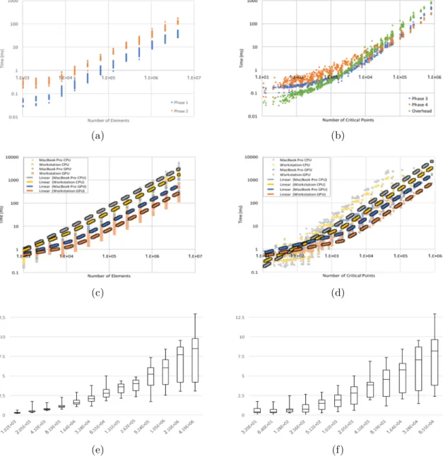
Figures 3.6(a) and 3.6(b) show log-log charts highlighting the performance of various phases of our approach. Figure 3.6(a) shows that in the average case, phases 1 and 2 grow linearly with respect to the number of elements in the field (R2 = 0.96 and R2 = 0.974, respectively). Similarly, Figure 3.6(b) shows that for the average case, phases 3, 4, and OpenCL overhead (data transfer, etc.) grows linearly with respect to the number of critical points in the field (R2 = 0.98, R2 = 0.992, and R2 = 0.992, respectively).
Figures 3.6(c) and 3.6(d) use log-log charts to compare the performance of our approach to the CPU implementation. Figure 3.6(c) shows the computational time against the
num-(a) (b)
(c) (d)
(e) (f)
Figure 3.6. Charts of the performance of our parallel merge tree algorithm on random fields. (a) Log-log chart of the processing time of Phase 1 and 2 is highly linear against the number of elements. (b) Log-log chart of processing time of Phase 3, 4, and overhead is highly linear against the number of critical points. (c) Log-log performance comparison of the number of elements against time and (d) the number of critical points against time. For both hardware configurations, the OpenCL implementation shows on average around 1 order of magnitude improvement over the CPU counterpart. (e) Log-linear boxplots of the speedup based upon the number of element and (f) based upon the number of critical points show that as the problem size grows, the speedup increases as well.
ber of elements, while Figure 3.6(d) shows the computational time against the number of critical points. The average time performance for both our algorithm and the conventional implementation is approximately linear. Our approach has the advantage of being highly parallel in nature. For both hardware configurations, our OpenCL implementation beat the CPU implementation by approximately one order of magnitude.
Figures 3.6(e) and 3.6(f) use log-linear charts to compare the speedup of our approach to the CPU implementation on the MacBook Pro. Figure 3.6(e) shows the speedup against the number of elements, while Figure 3.6(d) shows the speedup against the number of critical points. Interestingly, as the problem size grows, the GPU implementation speedup grows as well. We believe this is caused by the fact that the overall GPU performance is driven by the number of critical points, while the CPU performance is driven by the number of elements.
3.6.2 Contour Trees in Radio Astronomy Data
In radio astronomy, scalar fields are one of the primary data sources used to validate hy-potheses. Radio telescopes capture 3D maps of the radio signals in the sky. Two dimensions of these maps are spatial positions in the sky. The third dimension is different radio fre-quencies. Unfortunately for astronomers, the radio signals collected are very low power and have a low signal to noise ratio. The problem was described best by one radio astronomer, “a cell phone on the moon would be a brightest signal in the sky”.
Figure 3.7(a) shows an example of this data for a single radio frequency. The red blob towards the middle of the image is the feature of interest. In this dataset, this blob represents the signal put off by dust circling a black hole. For our experiments, we calculate the contour tree, which is just the union of a two merge trees (a join and split tree). Figure 3.7(b) shows a small region with the contour tree nodes highlighted. In this image, leaves can be seen (both local minima and maxima) as blueish purple nodes, and saddle points are yellow for join saddles and magenta for split saddles. Figure 3.8 shows the performance results for our
(a) (b)
Figure 3.7. Visualization of Radio Astronomy Data. (a) The noisy data shows the amplitude of the radio signal at multiple locations in the sky for a single wavelength. (b) The visual-ization of the contour tree shows the result of the union of a join tree with a split tree. The density of critical points in this data is quite high.
experiments. These experiments were only run on our MacBook Pro CPU/GPU. For each resolution (1024×1024, 2048×2048, and 4096×4096), we ran our tree construction on each of 38−2D slices (radio frequencies) of the data. Considered in our calculations are only the merge tree costs (i.e., no overhead). The log-log chart in Figure 3.8(a) shows that the time taken for our GPU implementation significantly outperforms the CPU implementation. Furthermore, both the CPU and GPU implementations performance grows linearly with the number of elements (R2 > 0.99). The log-linear boxplots in Figure 3.8(b) show the
speedup for our implementation. As the number of elements grows, so too does our speedup, reaching on average 40× faster for the GPU implementation on the 4096×4096 example. The speedup seen here is significantly better than that observed in the random field case. As mentioned in those tests, the random field example is the most challenging because of critical point density. For the random field tests, the median density was one critical point per 33.2 elements. For the radio astronomy data, the median density was one critical point
per 107.5 elements, over three times less dense. Given the strong relationship between the number of critical points and overall performance of our approach, this result makes sense.
(a) (b)
Figure 3.8. Performance on Radio Astronomy Data. Radio astronomy data (a) compute time and (b) speedup on the MacBook Pro CPU and GPU for 38 −2D slices at three different resolutions, 1024×1024 (1,048,576 elements), 2048 ×2048 (4,194,303 elements), and 4096×4096 (16,777,216 elements).
3.7 Conclusions
In conclusion, we have presented an approach for efficiently calculating merge trees in parallel by combining three approaches, pruning, spatial-domain parallelization, and value-domain parallelization. This approach makes it feasible to quickly calculate join trees, split trees, and contour trees for large scalar fields in any number of dimensions. These data structures are incredibly useful for analyzing scalar field data. We have evaluated our ap-proach with a synthetic random field dataset and with a dataset from the discipline of radio astronomy. Although we have calculated the merge tree in parallel, in the future, paralleliz-ing several additional computations would be exceedparalleliz-ingly useful. For example, parallelizparalleliz-ing the union of merge trees (the last step of building contour trees), calculating of persistence, or the hierarchical simplification of a join, split, and contour trees would all be very useful moving forward.
Chapter 4: Critical Point Pairing in Reeb Graphs
This chapter2 introduces efficient algorithms to pair critical points using persistent ho-mology.
4.1 Introduction
The last two decades have witnessed great advances in methods that rely on topologi-cal techniques to analyze data using Topologitopologi-cal Data Analysis (TDA). The popularity of topology-based techniques is due in large part to their robustness and their applicability to a wide variety of datasets and scientific domains [51]. The Reeb graph [63] was originally proposed as a data structure to encode the geometric skeleton of 3D objects, but recently it has been re-purposed as an important tool in TDA.
The Reeb graph encodes the evolution of level sets obtained from a scalar function by sweeping from negative infinity to positive infinity and tracking the birth and death of the connected components of the level sets.
Beside their usefulness in handling large data [34], Reeb graphs and their non-looping variant, contour trees [12], have been successfully used in image processing [45], data simplifi-cation [17, 68], feature detection [73], shape understanding [5], visualization of isosurfaces [6] and many other applications. One challenge with using Reeb graphs to directly analyze data is that the graph may still be too large or complex to directly visualize, therefore requiring further abstraction.
2Part of this chapter was published in Advances in Visual Computing (2019) [78]. Permission to reproduce
A fundamental tool in TDA is persistent homology, introduced by Edelsbrunner et al. [35]. Typically, persistent homology operates by transforming a point cloud data into a filtration (a nested sequence of spaces), performing persistent homology computation on the filtration, and parameterizing the obtained topological structures by their life-time in the filtration. As a result, persistent homology gives a topological description called the persistence diagram. The notion of persistence can be applied to any act of birth that is paired with an act of death. Since the Reeb graph encodes the birth and the death of the connected components of the level sets of a scalar function, the notion of persistence can be applied to pair the critical points in the Reeb graph [2].
Figure 4.1 shows an example of this analysis. Initially, a mesh with a scalar function (see Figure 4.1(a)) is converted into a Reeb graph (see Figure 4.1(b)). After that, the critical points are paired, and the persistence diagram displays the data, as seen in Figures 4.1(c) and 4.1(d). This final step can still be challenging, particularly when considering essential critical points—those critical points associated with cycles in the Reeb graph. These require an expensive search that needs to be performed on each essential critical point. While many prior works have provided efficient algorithms for the calculation of Reeb graph structures themselves, to our knowledge, none have provided a detailed description of an algorithm for pairing critical points.
In this chapter, we describe and implement two efficient algorithms to compute persis-tence diagrams from Reeb graphs. Our first algorithm uses a multi-pass approach that first pairs non-essential critical points using branch decomposition on join and split trees. It then pairs essential critical points using an approach also based upon join trees. Finally, this leads to our second approach, a new single-pass algorithm for pairing both non-essential and essential critical points in Reeb graphs.
G E D P I F L J K M H N O A B C A B G E D P C I F L J K M H N O
(a) Data with a scalar function
G E D P I F L J K M H N O A B C A B G E D P C I F L J K M H N O
(b) Reeb graph of the data P O N M L K J I H G F E D C B A A B G E C P N O K H A B C D E F G H I J K L M N O P B,C E,G O,N H,K
A,P Pd0of sublevel sets
Pd 0of su pe rle ve l s ets (c) Persistence diagram, Dg0(f) D F J H K1 K2 L,D J,F M,I P O N M L K J I H G F E D C B A A B C D E F G H I J K L M N O P (d) Extended persistence diagram, ExDg1(f)
Figure 4.1. Reeb graph and persistence diagram. Topological data analysis using Reeb graphs shows (a) data with a scalar function being processed into (b) a Reeb graph. Using the Reeb graph, critical points are then paired. (c) The persistence diagram, Dg0(f), and (d) extended persistence diagram, ExDg1(f), provide a visualization of the structures in the original data.
4.2 Reeb Graph
In Chapter 2 we introduced persistent homology and the persistence diagram. We also discussed critical point pairing of contour tree in an intuitive manner. Now we generalize the critical point pairing of the contour tree to the Reeb graph and provide a strict mathematical treatment of pairing in persistent homology.
We follow the terminology in Chapter 2. Let X be a triangulable topological space, and let f : X → IR be a continuous function defined on it. We define an equivalence class by the relation ∼on X, such thatx∼y, if and only if x and y belongs to the same connected component of f−1(r) for some r∈ IR. Given X and a function f :X →IR, the Reeb graph of X and f is the quotient spaceX/∼equipped with the quotient topology induced by the quotient mapπ:X →Rf(X). The Reeb graph is denoted byRf(X). WhenX is clear from
the context, we will denote the Reeb graph simply by Rf.
The Reeb graph can be thought of as a topological summary of the space X using the information encoded by the scalar function f. More precisely, the Reeb graph encodes the changes that occur to connected components of the level sets off−1(r) asrgoes from negative infinity to positive infinity. Figure 4.1 (a) and (b) shows an example of a Reeb graph defined on a surface.
The function ˜f can be used to classify points on the Reeb graph as follows. Let x be a point in Rf. Theup-degree of x is the number of branches incident tox which have greater
values of ˜f than x. The down-degree is defined similarly. A point x onRf is a critical point
if either its up-degree or down-degree is not equal to one. Otherwise it is a regular point. A critical point on the Reeb graph is also anode of Reeb graph. A critical point is a minimum or maximum if its down-degree or up-degree is equal to 0. Finally, a critical point is called a down-fork or up-fork if its down-degree or up-degree is greater than 1.
Without loss of generality, we assume that Reeb graph is a single connected component, and each node on Reeb graph has unique function value. Moreover, we assume also that every node in the Reeb graph is either a up-fork with up-degree 2, an fork with down-degree 2, a maximum, or a minimum. This is not a restriction to the general case, since a Reeb graph that does not satisfy these requirements can be conditioned to fit them, as we will show in Section 4.4.
4.2.1 Persistence Diagram of Reeb Graph
Of particular interest to us are the persistence diagram Dg0(f) and extended persistence diagram ExDg1(f). These two diagrams can be computed completely by considering the Reeb graph Rf. We give an intuitive explanation to this fact here, and we refer the reader
to [8] for more details.
Note that pairing of critical points of a scalar function can be computed independent of the computation of Reeb graphs. However, the pairing is best described using Reeb graph since the structure of Reeb graph clearly reveals the topological feature associated to the pairing.
Before we describe the points in the persistence diagram, Dg0(f), and extended persis-tence diagram, ExDg1(f), we need to distinguish between two types of forks in the Reeb graph, namely the ordinary forks and the essential forks. Let Rf be a Reeb graph and let o
be a down-fork such that r =f(o). We say that the down-fork o is an ordinary fork if the lower branches of o are not from the same connected component of (Rf)<r. The down-fork
o is said to be essential if it is not ordinary. The ordinary and essential up-forks are defined similarly.
4.2.1.1 Branching Features of Reeb Graph
We first consider pairing ordinary down-forks using sublevel set filtration. Letr∈R. We track changes that occur in H0((Rf)≤r) as r increases. A connected component of (Rf)≤r
is created when r passes through a minimum of Rf. Let C be a connected component of
(Rf)≤r. We say that a local minimum m of Rf creates C if m is the global minimum ofC.
Every ordinary down-fork is paired with a local minimum to form one point in the persistence diagram Dg0(f) as follows. Let o be an ordinary down-fork with f(o) = r and let C1 and C2 be the connected components of (Rf)<r. Let c1 andc2 be the creators ofC1 and C2, and
assume that f(c1) < f(c2). The homology class [c1+c2] that is born at f(c2) and dies at f(o) = r generates a point (c2, o) in the 0-th ordinary persistence diagram Dg0(f). Note
that such a pair occurs when the minimum is a branch in the Reeb graph, hence we name it a branching feature. Note also that we use critical points to represent the persistence pair, not the function values here.
Ordinary up-forks can be paired similarly by using superlevel set filtration. The pairing of each up-fork with a local maximum gives rise to points in the 0-th persistence diagram Dg0(f). For an ordinary up-fork, u, with f(u) = r, connected components C1 and C2 now
come from (Rf)>r. Letc1andc2 be the creators ofC1 andC2, and assume thatf(c1)< f(c2),
the homology class [c1 +c2] that is born at f(c1) dies at f(u) = r and generates a point
(c1, u) in Dg0(f).
4.2.1.2 Cycle Features of Reeb Graph
Let s be an essential down-fork with f(s) = r. We say s a creator of a 1-cycle in the sublevel set (Rf)≤r. As shown in [2],s will be paired with an essential up-forks0 to form an
essential pair (s0, s), a point in the extended persistence diagram ExDg1(f). The essential up-fork s0 is determined as follows. Let Γs be the set of all cycles born at s in the Reeb
graph Rf. We can pick the largest one among all the minimums of each cycle in Γs. Then
s0 is the point at which the function f achieves this largest minimum [8].
4.3 Related Work
Pairing of critical points of a scalar function has found multiple applications including segmentation of deformable shapes [71], hierarchical shape segmentation [64], description of protein shape [87], automatic extraction of surface structures [84], and 3D shape description and matching [11].
Branch decomposition was first used to provide a multiscale view of contour trees [59]. This provides the framework for pairing non-essential critical points in a Reeb graph. The first known description to pair critical points of a Morse function on a 2-manifold, including essential critical points, is given in [2]. However, the description is high level with no specific algorithm provided. Similar description of persistence pairing algorithm is also seen in [8].
To the best of our knowledge, this is the first systematic development and implementation of two intuitive and efficient algorithms to pair the nodes of Reeb graphs by persistent features.
4.4 Conditioning the Graph
As mentioned in Section 4.2.1, our approach is restricted to Reeb graphs where all point are either a minimum, maximum, up-fork with up-degree 2, or down-fork with down-degree 2. Fortunately, graphs that do not abide by these requirements can be conditioned to fit them. We define the J :K degree of a node as the J up-degree and K down-degree.
(a) Non-Critical (b) Degenerate Maximum (c) Double Fork (d) Complex Fork
Figure 4.2. Before pairing, the nodes of Reeb graph must be properly conditioned. There are four node configurations that require conditioning. New nodes and edges are shown in blue.
• 1:1 nodes—Nodes with both 1 up- and 1 down-degree are regular. Therefore, they only need to be removed from the graph. This is done by removing the regular point and reconnecting the nodes above and below, as seen in Figure 4.2(a).
• 0:2 (and 2:0) nodes—Nodes with 0 up-degree and 2 down-degree (or vice versa) are degenerate maximum (minimum) nodes, in that they are both down-fork (up-fork) and local maximum (minimum). As shown in Figure 4.2(b), this condition is corrected by added a new node for the local maximum higher value, where is a small number. This type of degenerate node rarely occurs in Reeb graphs, but it frequently occurs in approximations of a Reeb graph, such as Mapper [70].
• 2:2 nodes—Nodes with both 2 up- and 2 down-degree are degenerate double forks, both down-fork and up-fork. Figure 4.2(c) shows how double forks can be corrected by splitting into 2 separate forks, one up- and one down-fork, distance apart.
• 1:N>2 (and N>2:1) nodes—Nodes with down-degree (or up-degree) 3 or higher, are complex forks to pair. These are the forks corresponds to complex saddles inf, such as monkey saddles. A single critical point pairing to these forks just reduces the degree of down-fork by one, requiring complicated tracking of pairs. To simplify this, as seen in Figure 4.2(d), complex forks can be split into two forks apart. The upper down-fork retains one of the original down edges. The new down-fork connects with the old and takes the remaining down-edges. For even higher-order forks, the operation can be repeated on the lower down-fork.
Beyond these requirements, we assume the Reeb graph is a single connected component. If the Reeb graph contains multiple connected components, each one can simply be extracted and processed individually.
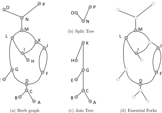
A B G E D P C I F L J K M H N O
(a) Reeb graph
P O N M L K J I H G F E D C B A A B G E C P N O K H A B C D E F G H I J K L M N O P B,C E,G N,O H,K A,P (b) Split Tree P O N M L K J I H G F E D C B A A B G E C P N O K H A B C D E F G H I J K L M N O P B,C E,G N,O H,K A,P (c) Join Tree D I F L J M (d) Essential Forks
Figure 4.3. Example of multipass critical point paring. In the multipass approach, (a) the Reeb graph has (b) a split tree and (c) a join tree extracted for non-essential pairing. Then in a separate process, the (d) essential forks are paired one at a time. The persistence diagram for this Reeb graph is shown in Figure 4.1(c) and 4.1(d).
4.5 Multipass Approach
Roughly speaking the Reeb graph gives rise to two types of topological features: the branching features and cy