Evolutionary many-objective optimisation: pushing the boundaries

(1)

Evolutionary Many-Objective Optimisation:

Pushing the Boundaries

Miqing Li

for the degree of Doctor of Philosophy of the

Department of Computer Science

Brunel University London

(2)

Declaration

I, Miqing Li, hereby declare that this thesis and the work presented in it is entirely my own. Some of the work has been previously published in journal or conference papers, and this has been mentioned in the thesis. Where I have consulted the work of others, this is always clearly stated.

(3)

(4)

Abstract

Many-objective optimisation poses great challenges to evolutionary algorithms. To start with, the ineffectiveness of the Pareto dominance relation, which is the most important criterion in multi-objective optimisation, results in the underperformance of traditional Pareto-based algorithms. Also, the aggravation of the conflict between proximity and diversity, along with increasing time or space requirement as well as parameter sensitivity, has become key barriers to the design of effective many-objective optimisation algorithms. Furthermore, the infeasibility of solutions’ direct observation can lead to serious difficulties in algorithms’ performance investigation and comparison. In this thesis, we address these challenges, aiming to make evolutionary algorithms as effective in many-objective optimisation as in two- or three-objective optimisation. First, we significantly enhance Pareto-based algorithms to make them suitable for many-objective optimisation by placing individuals with poor proximity into crowded regions so that these individuals can have a better chance to be eliminated. Second, we propose a grid-based evolutionary algorithm which explores the potential of the grid to deal with many-objective optimisation problems. Third, we present a bi-goal evolution framework that converts many objectives of a given problem into two ob-jectives regarding proximity and diversity, thus creating an optimisation problem in which the objectives are the goals of the search process itself. Fourth, we propose a comprehensive performance indicator to compare evolutionary algorithms in optimi-sation problems with various Pareto front shapes and any objective dimensionality. Finally, we construct a test problem to aid the visual investigation of evolutionary search, with its Pareto optimal solutions in a two-dimensional decision space having similar distribution to their images in a higher-dimensional objective space.

The work reported in this thesis is the outcome of innovative attempts at addressing some of the most challenging problems in evolutionary many-objective optimisation. This research has not only made some of the existing approaches, such as Pareto-based or grid-Pareto-based algorithms that were traditionally regarded as unsuitable, now effective for many-objective optimisation, but also pushed other important boundaries with novel ideas including bi-goal evolution, a comprehensive performance indicator

(5)

and a test problem for visual investigation. All the proposed algorithms have been systematically evaluated against existing state of the arts, and some of these algorithms have already been taken up by researchers and practitioners in the field.

(6)

Acknowledgement

First of all, I would like to express my deepest gratitude to my supervisors Prof. Xiaohui Liu and Prof. Shengxiang Yang for their great, persistent support and help on both my study and life during the four years. It is impossible to imagine better mentors for my PhD stage. Prof. Xiaohui Liu is very kind and always encourages, guides and helps me whenever and wherever I face difficulties. His kindness, encouragement, inspiration, and enthusiasm are invaluable during my whole PhD life. Prof. Shengxiang Yang is very responsible and strives for excellence. He has always made time to discuss my research and provided suggestions and hints to whatever problems I met. I was profoundly moved more than once by his rigorous scholarship.

I am truly grateful to my enlightenment teacher Prof. Jinhua Zheng, who has got me interested in scientific research, led me into the field of evolutionary computation, and given me continued support over these years.

Many thanks go to the people with whom I co-authored a number of papers during the period of my PhD study, namely Prof. Robert M. Hierons, Dr. Wei Zheng, Dr. Ser-gio Segura, Zhaomeng Zhu, Dr. Ke Li, Prof. Qingfu Zhang, Dr. Veronica Vinciotti, Prof. Jinhua Zheng, Dr. Ruimin Shen, and Kang Wang.

In addition, I would like to express my gratitude to the following people for use-ful discussions, suggestions, comments, and supports of my research during the PhD stage: Dr. Ruimin Shen, Prof. Zidong Wang, Liang Hu, Dr. Crina Grosan, Prof. Qingfu

Zhang, Ovidiu Pˆarvu, Kang Wang, and Zuofeng Zhang. I am also grateful to the

fol-lowing people or groups for providing their experimental data or opening their source codes for my research: Prof. Hisao Ishibuchi, Dr. Markus Wagner, Prof. Gary G. Yen, Prof. Kalyanmoy Deb, Prof. Qingfu Zhang, Dr. Tsung-Che Chiang, Dr. Evan J. Hughes, PISA, Jmetal, and OTL.

Further thank-yous are offered to my colleagues and friends from the Centre for Intelligent Data Analysis for the pleasant and enjoyable working atmosphere: Liang Hu, Chuang Wang, Dr. Djibril Kaba, Dr. Valeria Bo, Neda Trifonova, Izaz Rahman, Mohsina Ferdous, Dr. Emma Haddi, Dr. Zujian Wu, Dr. Yuanxi Li, Dr. Haitao Duan, Dr. Qian Gao, Dr. Ali Tarhini, Dr. Ana Salazar-Gonzalez. In addition, a special

(7)

thank-you goes to Ela Heaney for her kind help with everything at Brunel.

I would like to express my warmest thanks to my parents and my wife. My par-ents have always respected my choices and given me unconditional love, support and encouragement through all my life. My wife Su Guo, who had to go through difficult time to help me fulfil my dream, is so kind, patient, loving and caring and has provided tremendous support for my graduate study.

Finally, I would like to thank the Department of Computer Science, Brunel Univer-sity London for funding my four-year PhD research.

(8)

List of Figures

3.1 Evolutionary trajectories of the convergence metric (CM) for a run of

the original NSGA-II and the modified NSGA-II without the density

estimation procedure on the 10-objective DTLZ2. . . 74

3.2 An illustration of shift-based density estimation in a bi-objective

min-imisation scenario. To estimate the density of individual A, individuals

B,C, and D are shifted toB0,C0, andD0, respectively. . . 75

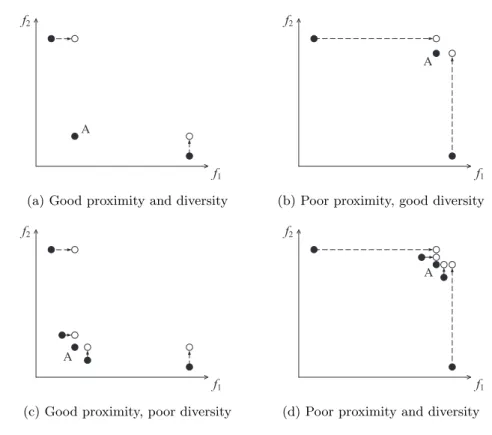
3.3 Shift-based density estimation for four situations of an individual (A) in

the population for a minimisation MOP. . . 76

3.4 An illustration of the three density estimators in traditional and

shift-based density estimation, where individual A is to be estimated in the

population. . . 78

3.5 Result comparison between NSGA-II and NSGA-II+SDE on the

10-objective DTLZ2. The final solutions of the algorithms are shown

re-garding the two-dimensional objective space f1 and f2. . . 81

3.6 Result comparison between SPEA2 and SPEA2+SDE on the 10-objective

TSP with T SP cp= 0. The final solutions of the algorithms are shown

regarding the two-dimensional objective spacef1 and f2. . . 83

3.7 Result comparison between PESA-II and PESA-II+SDE on the

10-objective DTLZ6. The final solutions of the algorithms are shown

re-garding the two-dimensional objective space f1 and f2. . . 86

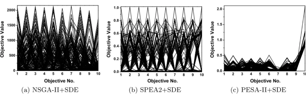
3.8 The final solution set of the three algorithms on the ten-objective DTLZ3,

(13)

3.9 An illustration of the failure of the crowding distance in TDE and SDE on a tri-objective scenario, showed by parallel coordinates. In a

nondom-inated set consisting ofA(1,1,1),B(0,10,2),C(2,0,10) andD(10,2,0),

individual A performs well in terms of proximity and diversity. But A

will be assigned a poor density value in both TDE and SDE since the

crowding distance separately considers its neighbours on each objective. 90

3.10 An illustration of the inaccuracy of the grid crowding degree. Dhas two

very close neighboursG and Hin SDE, but its grid crowding degree is

smaller than that of Cwhich has a relatively distant neighbour F. . . . 91

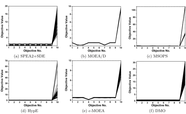
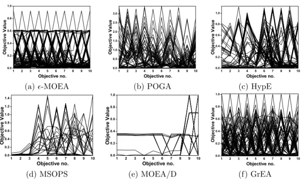
3.11 The final solution set of the six algorithms on the ten-objective DTLZ7,

shown by parallel coordinates. . . 95

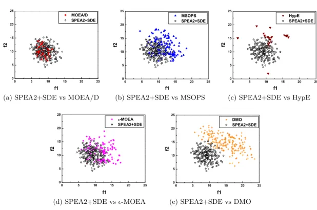
3.12 Result comparison between SPEA2+SDE and the other algorithms on

the 10-objective TSP with T SP cp = −0.2. The final solutions of the

algorithms are shown regarding the two-dimensional objective space f1

and f2. . . 97

4.1 An illustration of individuals in grid for a bi-objective scenario. . . 102

4.2 Setting of grid in the kth objective. . . 106

4.3 Illustration of fitness assignment. The numbers in the brackets

associ-ated with each solution correspond to GR and GCD, respectively. . . 110

4.4 A set of 4-objective individuals for archiving. The numbers in the

brack-ets correspond to their objective values. . . 117

4.5 An illustration of the environmental selection process. Individuals are

arranged in the order of their fitness values for observation. The framed individuals mean that they have entered the archive set. The archive size is set to 5. . . 118

4.6 Distribution of the solution set for the 4-objective example by parallel

coordinates. . . 119

4.7 The final solution set of the six algorithms on the ten-objective DTLZ2,

(14)

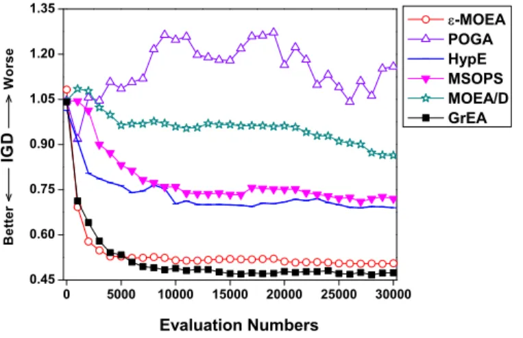
4.8 Evolutionary trajectories of IGD for the six algorithms on the ten-objective DTLZ2. . . 125

4.9 The final solution set of the six algorithms on DTLZ5(6,10), shown by

parallel coordinates. . . 130 4.10 Evolutionary trajectories of HV for the six algorithms on the five-objective

TSP, whereT SP cp=−0.2. . . 131

4.11 IGD of GrEA with different number of divisions on DTLZ2. . . 132 4.12 The final solution set of GrEA with different divisions on the six-objective

DTLZ2, shown by parallel coordinates. . . 133 4.13 The final solution set of GrEA with different divisions on the

three-objective DTLZ2, shown by Cartesian coordinates. . . 134

5.1 Evolutionary trajectories of the average convergence metric (CM) for 30

runs of the original NSGA-II (denoted asA) and the modified NSGA-II

without the diversity maintenance mechanism (denoted asA∗) on DTLZ2.139

5.2 An illustration of the conversion from the actual objective space to the

bi-goal space of proximity and crowding degree on a bi-objective min-imisation problem. . . 140

5.3 An illustration of the case that similar individuals in the objective space

may be located closely and nondominated to each other in the bi-goal space, and its remedy. (a) The actual objective space; (b) The bi-goal space with respect to the proximity and the original crowding degree; (c) The bi-goal space with respect to the proximity and the modified crowding degree. The numerical values of the individuals in these three spaces are given in Table 5.1. . . 144

5.4 The average number of solutions in all the nondominated layers under

(a) the bi-goal Pareto nondominated sorting and (b) the original Pareto nondominated sorting, where the population size is 100, the number of

runs is 30, and the test instance is DTLZ2. . . 147

5.5 The final solution set of the six algorithms on the ten-objective WFG9,

(15)

5.6 Result comparison between BiGE and each of the other five algorithms on the 15-objective TSP. The final solutions of the algorithms are shown

regarding the two-dimensional objective spacef1 and f2. . . 155

5.7 Normalised HV of the six algorithms with different settings of the

pop-ulation size on the 10-objective WFG9. . . 157

5.8 Normalised HV of the six algorithms with different settings of the

num-ber of objectives on WFG9. . . 158

6.1 An example that HV prefers the knee and boundary points on the Pareto

front, where two sets of Pareto optimal solutions on DTLZ2 are obtained by MOEA/D and IBEA. The solution set with better distribution (ob-tained by MOEA/D) has a worse (lower) HV result, as given in Table 6.1.167

6.2 An example that the unary additive -indicator fails to distinguish

be-tween two approximation sets. P andQhave the same evaluation result

(= 2.5). . . 168

6.3 An example that IGD and IGD+ fails to reflect the performance

differ-ence between approximation sets, where the referdiffer-ence set is constructed

by the approximation sets themselves. P andQhave the same IGD and

IGD+ evaluation results (0.884 and 0.625 respectively). . . 170

6.4 An example that the dominance distance of a set of solutions to a cluster

can be smaller than the minimum of their single dominance distance to

the cluster. For three sets P1, P2, and P3 (P1 ∈ C1, P2 ∈ C2, P3 ∈

C3, P = P1∪P2 ∪P3), their dominance distance to C1, C2 and C3 is

0.707, 0.559 and 0.0, respectively, while the minimum of their single

solution’s dominance distance to C1,C2 and C3 is 0.707, 1.031 and 1.0,

respectively. . . 174

6.5 Approximation sets of the six algorithms and their PCI result on the

modified tri-objective DTLZ1. . . 180

6.6 Approximation sets of the six algorithms and their PCI result on the

(16)

6.7 Approximation sets of the six algorithms in the two-variable decision space and their PCI result on the four-objective Rectangle problem, where the Pareto optimal solutions in the decision space are similar to their images in the objective space in the sense of Euclidean geometry. . 182

6.8 Parallel coordinate plot of approximation sets of the six algorithms and

their PCI result on the ten-objective DTLZ3. . . 183

7.1 An illustration of a four-objective distance minimisation problem whose

Pareto optimal region is determined by the four points. . . 188

7.2 An illustration of a Rectangle problem whose Pareto optimal region is

determined by the four lines. . . 189

7.3 The final solution set of the 15 algorithms on the Rectangle problem

wherex1, x2 ∈[−20,120]. . . 193

7.4 The final solution set of the five implementations of MOEA/D-PBI

with different penalty parameter values on the Rectangle problem where

x1, x2 ∈ [−20,120]. The number in the bracket denotes the penalty

parameter value of the algorithm. . . 194

7.5 The final solution set of the 15 algorithms on the Rectangle problem

wherex1, x2 ∈[−10000,10000]. . . 195

7.6 An illustration of the difficulty for algorithms to converge on the

Rect-angle problem. The shadows are the regions that dominate x1 and x2,

respectively. . . 197

7.7 The final solution set of the four algorithms on the Rectangle problem

(17)

List of Tables

2.1 Performance Indicators and their Properties . . . 42

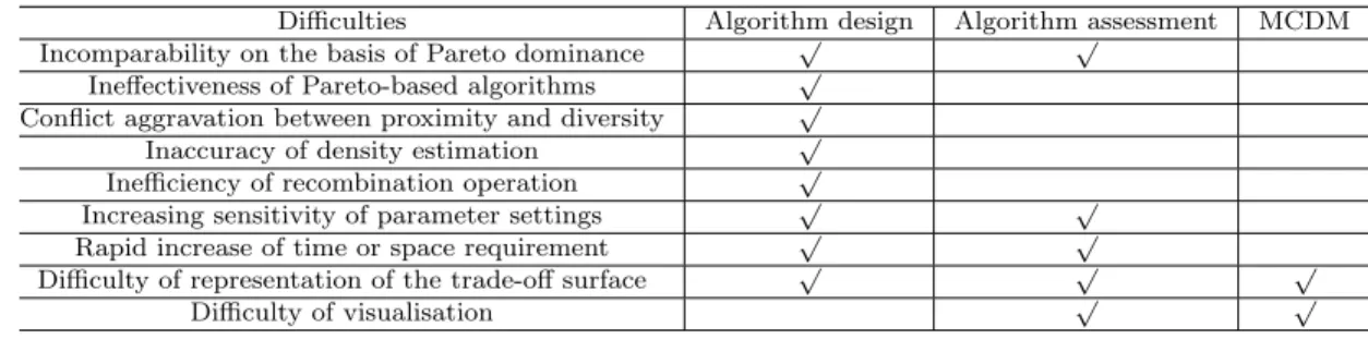
2.2 Difficulties in many-objective optimisation and their scope of the effect in

EMO, including algorithm design, algorithm assessment (investigation)

or/and multi-criteria decision making (MCDM). . . 50

3.1 Properties of test problems and parameter setting in II,

PESA-II+SDE, and -MOEA. The settings of div and correspond to the

different numbers of objectives of a problem. mandndenote the number

of objectives and decision variables, respectively . . . 79

3.2 Performance comparison between NSGA-II and NSGA-II+SDE

regard-ing the mean and standard deviation (SD) values on the DTLZ and TSP test suites, where IGD was used for DTLZ and HV for TSP. The better result regarding the mean for each problem instance is highlighted in

boldface . . . 82

3.3 Performance comparison between SPEA2 and SPEA2+SDE regarding

the mean and standard deviation (SD) values on the DTLZ and TSP test suites, where IGD was used for DTLZ and HV for TSP. The better result regarding the mean for each problem instance is highlighted in

(18)

3.4 Performance comparison between PESA-II and PESA-II+SDE regard-ing the mean and standard deviation (SD) values on the DTLZ and TSP test suites, where IGD was used for DTLZ and HV for TSP. The better result regarding the mean for each problem instance is highlighted in

boldface . . . 85

3.5 Performance comparison (mean and SD) of NSGA-II+SDE, SPEA2+SDE,

and PESA-II+SDE on the DTLZ and TSP test suites, where IGD was used for DTLZ and HV for TSP. The best result regarding the mean value among the three algorithms for each problem instance is

high-lighted in boldface . . . 87

3.6 IGD results (mean and SD) of the six algorithms on the DTLZ problems.

The best result regarding the mean IGD value among the algorithms for

each problem instance is highlighted in boldface . . . 93

3.7 HV results (mean and SD) of the six algorithms on the TSP problems.

The best result regarding the mean HV value among the algorithms for

each problem instance is highlighted in boldface . . . 96

4.1 Settings of the test problems . . . 120

4.2 Parameter settings in GrEA and -MOEA, where m is the number of

objectives . . . 121

4.3 IGD results of the six algorithms on DTLZ2, DTLZ4, DTLZ5, and DTLZ7123

4.4 IGD results of the six algorithms on DTLZ1, DTLZ3, and DTLZ6 . . . 126

4.5 IGD results of the six algorithms on DTLZ5(I, m), wherem= 10. . . . 128

4.6 HV results of the six algorithms on the multi-objective TSP. . . 129

4.7 Performance of GrEA with different number of divisions on the

six-objective DTLZ2 . . . 133

5.1 Individual values in the three spaces for the example of Figure 5.3. . . . 144

(19)

5.3 Normalised HV results (mean and SD) of the six algorithms on the WFG problem. The best and the second mean among the algorithms for each problem instance is shown with dark and light grey background, respectively . . . 151

5.4 Normalised HV results (mean and SD) of the six algorithms on the

Knapsack problem. The best and the second mean among the algorithms for each problem instance is shown with dark and light grey background, respectively . . . 153

TSP problem. The best and the second mean among the algorithms for each problem instance is shown with dark and light grey background, respectively . . . 154

water problem. The best and the second mean among the algorithms for each problem instance is shown with dark and light grey background, respectively . . . 156

5.7 Normalised HV of BiGE with different settings of the sharing

discrimi-nator on the 10-objective WFG9. . . 159

5.8 Normalised HV of BiGE with the settings of the sharing discriminator

that only discourage the individual with worse proximity on the 10-objective WFG9. . . 159

5.9 Normalised HV results (mean and SD) of the four algorithms on all the

34 test instances. The best and the second mean among the algorithms for each problem instance is shown with dark and light grey background, respectively . . . 162

6.1 HV results of the two sets in Figure 6.1 under different reference points.

The range of DTLZ2’s Pareto front is [0,1] for all objectives. . . 168

(20)

6.3 Evaluation results of PCI and the peer indicator (HV, -indicator, or

IGD+) on the approximation set instances in Figures 6.1–6.3. The

ref-erence point 1.1 is used in the HV calculation of Figure 6.1’s instance.

A better result is highlighted in boldface. . . 179

(21)

Nomenclature

Acronyms

ASF achievement scalarizing function

CM convergence measure

DM decision-maker

DTLZ Deb, Thiele, Laumanns and Zitzler test suite

EaMO evolutionary many-objective optimisation

EMO evolutionary multi-objective optimisation

GCD grid crowding distance

GCPD grid coordinate point distance

GR grid ranking

HV hypervolume indicator

IGD inverted generational distance

MCDM multi-criteria decision making

MOP multi-objective optimisation problem

MaOP many-objective optimisation problem

PCA principle component analysis

PCI performance comparison indicator

ROI region of interest

SBX simulated binary crossover

SOP single-objective optimisation problem

TSP travelling salesman problem

UF unconstrained function

WFG walking fish group test suite

(22)

Algorithms

AGE-II approximation-guided evolutionary algorithm

AR average ranking

AR+Grid average ranking combined with grid

BiGE bi-goal evolution

DMO diversity management operator

EA evolutionary algorithm

-MOEA -dominance based MOEA

FD-NSGA-II fuzzy dominance-based NSGA-II

GrEA grid-based evolutionary algorithm

HypE hypervolume estimation algorithm

IBEA indicator based evolutionary algorithm

MOEA multi-objective evolutionary algorithm

MOEA/D multi-objective evolutionary algorithm based on decomposition

MOEA/D+PBI MOEA/D with penalty boundary intersection function

MOEA/D+TCH MOEA/D with Tchebycheff function

MSOPS multiple single objective Pareto sampling

NSGA-II non-dominated sorting genetic algorithm II

NSGA-II+SDE NSGA-II with shift-based density estimation

NSGA-III non-dominated sorting genetic algorithm III

PESA-II Pareto envelope-based selection algorithm II

PESA-II+SDE PESA-II with shift-based density estimation

POGA preference order based genetic algorithm

SDE shift-based density estimation

SMS-EMOA S-metric selection based EMO algorithm

SPEA2 strength Pareto evolutionary algorithm 2

(23)

Symbols

div number of divisions in the grid

fi theith objective value

Gi grid coordinate in the ith objective

m number of objectives

n number of decision variables

N population size

P evolutionary population (solution set)

pc crossover probability

pm mutation probability

Q archive set

Rn field of real numbers

T SPcp correlation parameter in TSP

xi theith decision variable

ηc distribution index in SBX crossover

ηm distribution index in polynomial mutation

(24)

Chapter 1

Introduction

An individual would like to maximise the chance of being healthy and wealthy while still having fun and time for family and friends. A software engineer would be inter-ested in finding the cheapest test suite while achieving full coverage (e.g., statement coverage, branch coverage and decision coverage). When prescribing radiotherapy to a cancer patient, a doctor would have to balance the attack on tumour, potential im-pact on healthy organs, and the overall condition of the patient. These multi-objective optimisation problems (MOPs) can be seen in various fields, sharing the same issue of pursuing several, often conflicting, objectives at the same time.

In MOPs, due to the conflicting nature of objectives, there is usually no single optimal solution but rather a set of alternative solutions, known as Pareto optimal solutions. These solutions are optimal in the sense that there are no other solutions in the search space that are superior for all objectives considered.

Evolutionary algorithms (EAs) are a class of stochastic optimisation methods that simulate the process of natural evolution. EAs have been recognised to be well suited for MOPs due to its characteristics of 1) low requirements on the problem properties, 2) being capable of handling large and highly complex search spaces, and particularly 3) population-based property which can search for a set of solutions in a single optimisa-tion run, each representing a particular performance trade-off amongst the objectives. As a subcategory of MOPs, many-objective optimisation problems (MaOPs) refer to an optimisation problem having four or more objectives. Over the last decade,

(25)

many-1.1. Motivation 1. Introduction

objective optimisation has been gaining rapidly increasing attention in the evolutionary computation community, driven by a wide variety of real-world applications (see [168]). However, there exists great difference between many-objective optimisation and two- or three-objective optimisation. Major challenges lie in the way of the use of EAs to deal with MaOPs. In this thesis, we present a number of approaches to address these challenges, paving the way for the effective use of EAs in many-objective optimisation. In this chapter, we first explain the motivation that led to the undertaking of this research, then we outline the main contributions of our work and the overall structure of this thesis, and finally we detail the publications which have resulted from the thesis.

1.1

Motivation

Since the early 90s, evolutionary multi-objective optimisation (EMO) algorithms1 have

demonstrated their effectiveness in solving various two- or three-objective optimisation problems. However, in practice, it is not uncommon to face an optimisation problem with four or more objectives (sometimes up to 10 or 15 objectives). Thus, it is not surprising that handling MaOPs has been one of the main research activities in the EMO area during the past few years.

Many-objective optimisation poses a number of challenges to EMO algorithms. Most notably, the Pareto dominance relation, which is the most important criterion in multi-objective optimisation, loses its effectiveness to differentiate individuals (solu-tions) in many-objective optimisation [74, 50, 67]. This makes EMO algorithms that work under the principle of Pareto dominance fail to provide selection pressure towards the Pareto front (i.e., Pareto optimal solutions in the objective space) [216, 256, 128]. In these algorithms, the density-based selection criterion will play a leading role in determining the survival of individuals in the evolutionary process, thus resulting in the final individuals distributed widely over the objective space but distant from the desired Pareto front. In fact, some studies have shown that a random search algorithm may even achieve better results than Pareto-based algorithms in problems with around 10 objectives [216, 152, 164].

(26)

1.1. Motivation 1. Introduction

In multi-objective optimisation, an EMO algorithm pursues two basic but often conflicting goals, proximity (also called convergence in some literature) and diversity. Such conflict has a detrimental impact on an algorithm’s optimisation process and

is particularly aggravated in many-objective optimisation [216, 1]. The algorithms

capable of achieving a good balance between proximity and diversity in two- or three-objective problems could easily fail in many-three-objective optimisation [256, 138, 88]. In addition, a high objective dimensionality can also give rise to difficulty for the crowding evaluation [162, 52], parameter settings [216, 88, 180], and data structure used in EMO algorithms [45, 256]. All of these bring a big challenge for the design of new algorithms in many-objective optimisation.

Performance assessment is an important issue in evolutionary many-objective op-timisation. However, many performance indicators, which are designed in principle for any number of objectives, are invalid or infeasible in practice to be used in many-objective optimisation [174, 254]. For example, indicators which is based on Pareto dominance relation typically return undifferentiated results of two solution sets with high dimensions. Indicators whose time or space requirement exponentially increases with the number of objectives may not be suitable for many-objective optimisation. Indicators which require a substitution of the Pareto front (as a reference set for com-parison) could become inaccurate since it is very hard to properly represent a high-dimensional Pareto front.

Finally, a visual observation of the population becomes difficult in many-objective optimisation. Even though some effort has been made along this line (see [259, 249]), there is still a lack of simple, intuitive way to visualise solutions in the objective space with four or more objectives. This directly affects the algorithm analysis and investi-gation and also subsequent decision-making process.

Overall, the above challenges cause great difficulties in the use of classic Pareto-based algorithms in many-objective optimisation, in the design of new algorithms for many-objective problems, in the assessment of solution sets obtained by many-objective optimisers, and in the visualisation of solutions in a high-dimensional space. All of these suggest the pressing need of new methodologies for evolutionary many-objective

(27)

1.2. Contributions 1. Introduction

optimisation.

With these in mind, this thesis explores a number of innovative approaches to ad-dress these challenges in evolutionary many-objective optimisation, including a general enhancement of Pareto-based algorithms to make them suitable for many-objective op-timisation (Chapter 3), an evolutionary algorithm which exploits the potential of the grid in objective optimisation (Chapter 4), an optimisation framework for many-objective problems (Chapter 5), a performance indicator for assessing solution sets with any number of objectives (Chapter 6), and a test problem for visual investigation of high-dimensional evolutionary search (Chapter 7). In short, our aim is to make EAs be considered as an effective tool in many-objective optimisation as in low-dimensional multi-objective (i.e., two- or three-objective) optimisation.

1.2

Contributions

The main contributions of the thesis are listed as follows.

• We significantly enhance Pareto-based algorithms by introducing a shift-based

density estimation (SDE) to make them suitable for many-objective problems (Chapter 3). Unlike most of the current work which typically relaxes the Pareto dominance relation to make more individuals comparable, SDE works on the den-sity estimation operation in Pareto-based algorithms. In view of the preference of density estimators for individuals in sparse regions, SDE “puts” individuals with poor proximity into crowded regions. This way, these poorly-converged in-dividuals will be assigned a high density value, thus having a better chance to be eliminated in the diversity maintenance process of Pareto-based algorithms. The implementation of SDE is very simple, with negligible computational cost, and it can be applied to any Pareto-based algorithm without the need of additional parameters.

The application of SDE in three popular Pareto-based algorithms has shown its high effectiveness in many-objective optimisation, especially when working with an accurate density estimator. Furthermore, from a comprehensive comparison

(28)

with five state-of-the-art algorithms, SDE has been demonstrated to be very com-petitive in finding a well-converged and well-distributed solution set on various

many-objective optimisation problems with up to 10 objectives2.

• We propose a novel algorithm, GrEA, to deal with many-objective optimisation

problems (Chapter 4). GrEA explores the potential of the use of the grid in many-objective optimisation. Specifically, a set of grid-based criteria are intro-duced to guide the search towards the optimal front, and a grid-based fitness adjustment strategy is proposed to maintain an extensive and uniform distribu-tion among individuals. In particular, to measure the crowding of individuals, GrEA considers the distribution of their neighbours in a set of hyperboxes whose size increases with the number of objectives, thus providing an accurate evalua-tion of individuals’ crowding degree.

From systematic experiments on 52 test instances with many objectives, GrEA has demonstrated its effectiveness in balancing proximity and diversity. Moreover, an appealing property of the algorithm is that its computational cost is almost independent on the number of hyperboxes in the grid and only increases linearly with the number of objectives. This is against the commonly accepted view [45] that grid-based approaches are not suitable in many-objective optimisation given their operation relying on the hyperboxes that exponentially grow in size with the number of objectives.

• We propose a bi-goal evolution (BiGE) framework for addressing many-objective

optimisation problems (Chapter 5). Inspired by two observations: 1) the con-flict between proximity and diversity is aggravated with the increase of objective dimensionality and 2) the Pareto dominance loses its effectiveness for a high-dimensional space but works well on a low-high-dimensional space, BiGE converts a given many-objective optimisation problem into a bi-goal (objective) optimisa-tion problem regarding proximity and diversity, and then handles it using the Pareto dominance relation in this bi-goal domain.

(29)

Systematic experiments are carried out to compare BiGE with five state-of-the-art algorithms on three groups of continuous and combinatorial benchmark suites with 5 to 15 objectives as well as on a real-world problem. In contrast to its com-petitors which work well on only a fraction of the test problems, BiGE can achieve a good balance between individuals’ proximity and diversity on the problems with various properties.

• We propose a novel performance comparison indicator (PCI) to assess solution

sets obtained by stochastic search algorithms in multi-objective optimisation (Chapter 6). In doing so, we also make a detailed analysis of the difficulties of popular performance indicators encountering in many-objective optimisation. PCI provides a comprehensive assessment of solution sets’ proximity and diver-sity, and it can be used in problems with various Pareto front shapes and any objective dimensionality. In contrast to current state of the art, PCI is par-ticularly practical in many-objective optimisation, given its characteristics of 1) no need for a specified reference set, 2) quadratic time complexity, 3) providing higher selection pressure than Pareto dominance but still being compliant with the latter, and 4) no requirement of parameter setting in the assessment.

• Finally, we construct a test problem (called Rectangle problem) to aid the visual

investigation of multi-objective search (Chapter 7). Key features of the Rectangle problem are that the Pareto optimal solutions 1) lie in a rectangle in the two-variable decision space and 2) are similar to their images in the four-dimensional objective space (in the sense of Euclidean geometry). In this case, it is capable of visually examining the behaviour of objective vectors in terms of both prox-imity and diversity, by observing their closeness to the optimal rectangle and their distribution in the rectangle, respectively, in the decision space. Fifteen well-established algorithms are investigated on the Rectangle problem. Inter-estingly, most state-of-the-art algorithms (including those designed specially for many-objective optimisation) struggle on this relatively low-dimensional problem (having only 4 objectives). This indicates that the Rectangle problem can also be

(30)

1.3. Thesis Structure 1. Introduction

used as a challenging benchmark function to test algorithms’ ability in balancing proximity and diversity.

Altogether, these five contributions represent a significant advance in evolutionary many-objective optimisation, which should provide considerable help for researchers and practitioners in both algorithm development and problem solving. When design-ing a Pareto-based algorithm, researchers only need to focus on tackldesign-ing two- or three-objective problems; for an optimisation problem with many three-objectives, SDE (Chap-ter 3) could be easily used. When working out a many-objective algorithm, the de-veloper can use the Rectangle problem (Chapter 7) to investigate the behaviour of the algorithm or/and the PCI indicator (Chapter 6) to assess the performance of the algorithm. When dealing with a many-objective problem in hand, the user can di-rectly adopt the algorithm GrEA (Chapter 4) or design new proximity and diversity estimation methods under the bi-goal evolution framework (Chapter 5).

1.3

Thesis Structure

This thesis is organised as follows.

Chapter 2 provides the necessary background material for the thesis. Beginning with the basic concepts in multi-objective optimisation, the chapter introduces key parts of EMO, including algorithm components, mainstream methods, test problems, and performance indicators. Then, general issues on many-objective optimisation are introduced, with a particular focus on the difficulties in many-objective optimisation and visualisation approaches in a high-dimensional space. Finally, various evolutionary many-objective optimisation techniques are described from different perspectives of addressing MaOPs.

Starting by the motivation of the work, Chapter 3 introduces a general enhancement of density estimation in Pareto-based algorithms to make them suitable for many-objective problems. SDE is integrated into three popular Pareto-based algorithms, NSGA-II, SPEA2 and PESA-II. Three groups of experiments are carried out to sep-arately investigate 1) whether SDE improves the performance of all the three

(31)

Pareto-1.3. Thesis Structure 1. Introduction

based algorithms, 2) among the density estimators in NSGA-II, SPEA2 and PESA-II which one is most suitable for SDE, and 3) how Pareto-based algorithms, when inte-grated with SDE, compare with other state-of-the-art algorithms designed specially for MaOPs.

Chapter 4 begins with the motivation of the use of grid in many-objective optimi-sation. Then, three grid-based fitness criteria are introduced, followed by their use in the mating selection and environmental selection processes. Finally, the performance of GrEA is empirically verified in sequence by the comparative study, parameter inves-tigation, and algorithm analysis.

In Chapter 5, we propose a bi-goal evolution framework for many-objective prob-lems. We first give the motivation of this work and then detail the BiGE framework and its implementation. This implementation includes four parts: proximity estimation, di-versity estimation, mating selection, and environmental selection. Next, experimental results of BiGE in comparison with five best-in-class algorithms are shown, and fi-nally a further investigation is provided to verify the proposed framework as well as its implementation.

The above three chapters present three approaches to deal with many-objective op-timisation problems. In Chapter 6, we suggest a performance indicator to assess many-objective optimisation approaches. We first review related works in multi-many-objective optimisation and analyse their difficulties in many-objective optimisation. Then, we detail the proposed indicator. Finally, two classes of comparative studies are conducted to analytically and empirically verify PCI, respectively.

Chapter 7 focuses on another important issue in many-objective optimisation: vi-sual investigation of multi-objective search. There, we present a test problem whose Pareto optimal solutions in the 2D search space have a similar distribution to their im-ages in the 4D objective space. The proposed problem is tested by 15 EMO algorithms, with three instances of the problem to provide different challenges for these algorithms in balancing proximity and diversity.

In Chapter 8, we summarise the work presented in this thesis and look at how this has contributed to the field of evolutionary many-objective optimisation. Furthermore,

(32)

1.4. Publications 1. Introduction

we suggest several directions of future research which have arisen during the course of this thesis.

1.4

Publications

The work resulting from this thesis has been published in the following papers:

• M. Li, S. Yang, and X. Liu. Bi-goal evolution for many-objective optimization

problems. Artificial Intelligence, 228: 45–65, 2015.

(Resulting from Chapter 5)

• M. Li, S. Yang and X. Liu. A performance comparison indicator for Pareto

front approximations in many-objective optimization. In Proceedings of the 17th Annual Conference on Genetic and evolutionary computation (GECCO), 703– 710, 2015, ACM.

• M. Li, S. Yang, and X. Liu. Shift-based density estimation for Pareto-based

algorithms in many-objective optimization. IEEE Transactions on Evolutionary Computation, 18(3): 348–365, 2014.

• M. Li, S. Yang, and X. Liu. Diversity comparison of Pareto front

approx-imations in many-objective optimization. IEEE Transactions on Cybernetics, 44(12): 2568–2584, 2014.

(Resulting from Chapters 2 and 6)

• M. Li, S. Yang, and X. Liu. A test problem for visual investigation of

high-dimensional multi-objective search. In Proceedings of IEEE Congress on

Evo-lutionary Computation (CEC), 2140–2147, 2014, IEEE. (Best Student Paper

Award)

(33)

• S. Yang, M. Li, X. Liu, and J. Zheng. A grid-based evolutionary algorithm for

many-objective optimization. IEEE Transactions on Evolutionary Computation, 17(5): 721–736, 2013.

• M. Li, S. Yang, X. Liu, and R. Shen. A comparative study on evolutionary

algo-rithms for many-objective optimization. In Proceedings of the 7th International Conference on Evolutionary Multi-Criterion Optimization (EMO), 261–275, 2013, Springer.

In addition to the above, other papers, produced during the course of my PhD research, can be seen as indirect results of the research discussed in this thesis, as listed below. They have either focused on the algorithm development of evolutionary multi-objective optimisation or applied multi- or many-multi-objective evolutionary approaches (including some presented in this thesis) to real-world problems.

• M. Li, S. Yang, and X. Liu. Pareto or non-Pareto: Bi-criterion evolution in

multi-objective optimization. IEEE Transactions on Evolutionary Computation, 2015, in press.

• Z. Zhu, G. Zhang, M. Li, and X. Liu. Evolutionary multi-objective workflow

scheduling in cloud. IEEE Transactions on Parallel and Distribution Systems, 2015, in press.

• W. Zheng, R. Hierons, M. Li, X. Liu, V. Vinciotti. Multi-objective optimisation

for regression testing. Information Sciences, 2015, in press.

• M. Li, S. Yang, J. Zheng, and X. Liu. ETEA: A Euclidean minimum spanning

tree-based evolutionary algorithm for multiobjective optimization. Evolutionary Computation, 22(2): 189–230, 2014.

(34)

• M. Li, S. Yang, K. Li, and X. Liu. Evolutionary algorithms with segment-based

search for multiobjective optimization problems. IEEE Transactions on Cyber-netics, 44(8): 1295–1313, 2014.

• K. Li, Q. Zhang, S. Kwong, M. Li, R. Wang. Stable matching based selection

in evolutionary multiobjective optimization. IEEE Transactions on Evolutionary Computation, 18(6): 909–923, 2014.

• M. Li, S. Yang, X. Liu, and K. Wang. IPESA-II: Improved Pareto

envelope-based selection algorithm II. In Proceedings of the 7th International Conference on Evolutionary Multi-Criterion Optimization (EMO), 143–155, 2013, Springer.

• R. Hierons, M. Li, X. Liu, S. Segura, and W. Zheng. An improved method for

optimal product selection from feature models. ACM Transactions on Software Engineering and Methodology, under review.

(35)

Chapter 2

Background

This chapter provides a review of evolutionary multi- and many-objective optimisation. The literature on this particular topic is vast and we will highlight the most relevant to this study.

This chapter is organised as follows. In Section 2.1, we present basic concepts in multi-objective optimisation, and this is followed by the description of key parts in EMO in Section 2.2. Section 2.3 introduces many-objective optimisation, with particular focuses on the difficulties of EMO algorithms in many-objective optimisation and the visualisation of solutions in a high-dimensional space. Finally, Section 2.4 provides a thorough review of evolutionary approaches for many-objective optimisation.

2.1

Basic Concepts

In general, a multi-objective optimisation problem (MOP) includes a set of ndecision

variables, a set ofm objective functions, a set ofJ inequality constraints, and a set of

(36)

2.1. Basic Concepts 2. Background

the following form:

Minimize fj(x), j = 1,2, ..., m

Subject to gj(x)≤0, j = 1,2, ..., J

hk(x) = 0, k= 1,2, ..., K

Li ≤xi ≤Ui, i= 1,2, ..., n

(2.1)

where x is a vector of n decision variables: x = (x1, x2, ..., xn), x ∈ Rn. The last

constraint set is called variable bounds, restricting each decision variablexi within the

range of [Li, Ui]. In an MOP, feasible solutions (denoted as x ∈ Rnf) refer to those

solutions which satisfy all inequality and equality constraints. In the following, we introduce some underlying concepts in multi-objective optimisation.

Definition 2.1.1 (Pareto dominance). For two decision variables x and y, x is said

to Pareto dominate y (denoted asx≺y), if and only if

∀i∈(1,2, ..., m) :fi(x)≤fi(y) ∧

∃j∈(1,2, ..., m) :fj(x)< fj(y)

(2.2)

Pareto dominance reflects the weakest assumption about the preference of the deci-sion maker; a solution is always preferable to another solution if the former dominates the latter. Accordingly, those solutions that are not dominated by any other solution

are denoted as Pareto optimal. Pareto optimal solutions are characterised by the fact

that improving in any one objective means worsening at least one other objective. The

set of Pareto optimal solutions in the decision space is denoted as thePareto set, and

the corresponding set of objective vectors is denoted as thePareto front. Next, we give

the formal definition of these concepts.

Definition 2.1.2 (Pareto optimality). A solution x∈Rnf is said to be Pareto optimal

if and only if @y∈Rnf, y≺x.

Definition 2.1.3 (Pareto set). The Pareto set (PS) is defined as the set of all Pareto

optimal solutions, namely, P S={x∈_Rn

(37)

2.2. Evolutionary Multi-Objective Optimisation 2. Background

Definition 2.1.4(Pareto front). The Pareto front (PF) is defined as the set of all

ob-jective vectors corresponding to the solutions in PS, namely,P F ={(f1(x), ..., fm(x)) :

x∈P S}.

Note that the size of the Pareto optimal solutions might be infinite and it is often infeasible to obtain the whole Pareto front. In practice, we want to obtain an approxi-mation of the Pareto front that contains as much inforapproxi-mation as possible of the Pareto front, so the decision maker can either choose one element of the approximation as the final solution, or use this information to specify preferences that help search and find a satisfied solution.

2.2

Evolutionary Multi-Objective Optimisation

This section introduces some key parts in EMO, including algorithm components tion 2.2.1), mainstream EMO methods (Section 2.2.2), performance indicators (Sec-tion 2.2.3), and test problems (Sec(Sec-tion 2.2.4).

2.2.1 Introduction

Evolutionary algorithms (EAs) stand for a class of stochastic search and optimisation methods that mimic the process of natural evolution. Over the past two decades, there has been significant interest in the use of EAs to solve MOPs (usually called evolu-tionary multi-objective optimisation (EMO) algorithms or multi-objective optimisation algorithms (MOEAs)), with success in fields as diverse as engineering, physics, chem-istry, biology, economics, marketing, operations research, and social sciences [50, 41, 40, 285, 209]. This can be attributed to two major advantages of EAs. One is that they have low requirements on the problem characteristics and are capable of handling large and highly complex search spaces. The other is that their population-based search can achieve an approximation of the problem’s Pareto front, with each solution representing a particular trade-off amongst the objectives.

The goal of approximating the Pareto front is itself multi-objective. In general, an EMO algorithm, in the absence of any further information provided by the decision

(38)

maker, pursues two ultimate goals with respect to its solution set – minimising the distance to the Pareto front (i.e., proximity or convergence) and maximising the distri-bution over the Pareto front (i.e., diversity). These two goals run through the design of all components of an EMO algorithm.

In the following, we briefly introduce several components of an EMO algorithm which are closely related to this thesis: fitness assignment, diversity maintenance, and selection; of course, other components are also crucial, such as variation, population initialisation, and stop criterion of an evolutionary algorithm.

Fitness Assignment

In contrast to single-objective optimisation in which the objective function and fit-ness function are typically identical, fitfit-ness assignment in multi-objective optimisation must allow for several goals. Many EMO algorithms design the fitness function on the basis of the Pareto dominance relation in the sense that the information of indi-viduals dominating, being dominated or nondominated is used to define a rank, such as dominance count, dominance rank, strength, and others [50, 19, 43]. In addition, since Pareto dominance fails to reflect the diversity of individuals in a population, density information is also recognised as an auxiliary consideration to incorporate into the fitness function. This enables the population to evolve towards the optimum and simultaneously to diversify its individuals uniformly along the trade-off front.

Recently, there has been increasing interest in the use of other criteria (instead of Pareto dominance) in fitness assignment, with the aggregation-based criterion and indicator-based criterion being important examples. Typically, they convert an objec-tive vector into a scalar value, thus providing a totally-ordered set of individuals in the population. Compared with Pareto dominance, such criteria have clear advantages, e.g., providing higher selection pressure towards the Pareto front [17, 138] and being easier to work with local search techniques stemming from global optimisation [169, 13].

Diversity Maintenance

Most EMO algorithms try to maintain diversity by incorporating density infor-mation into the selection process (often for nondominated individuals): the higher the

(39)

density of the surrounding area of an individual in the population, the lower the chance

of the individual being selected. At the beginning, the niching technique, introduced

by Goldberg [86], has been used to estimate the crowding degree of individuals in a population. With the development of the area, more density estimation methods, along with new EMO algorithms, have been presented. Among them, the cluster [294],

crowding distance [55, 205], k-th nearest neighbour [292, 62], grid crowding degree

[44, 150, 273, 181], and harmonic crowding distance [266] are representative examples. On the other hand, some EMO algorithms maintain diversity of a population from other perspectives, for example, by integrating proximity and diversity into a single cri-terion [291] or by decomposing an MOP into a number of scalar optimisation problems with a set of well-distributed weight vectors [278]. These methods have been found to be very effective on some MOPs [17, 278]. However, since they are not completely in line with individuals’ density in the population, their performance may be dependant on the shape of the Pareto front of an MOP at hand to some extent [179].

Selection

In the evolutionary process, selection represents the competition for resources among individuals. Some individuals better than others are naturally more likely to survive and to reproduce their genetic information. According to this principle, the overall se-lection operation in EMO algorithms can be split into two processes, mating sese-lection (i.e., selection for variation) and environmental selection (i.e., selection for survival) [215]. Mating selection aims at picking promising individuals for variation and is usu-ally performed in a random way. Environmental selection determines which of the previously stored individuals and the newly created ones are preserved in the archive (or the next population) and is usually performed in a deterministic way.

Interestingly, most EMO algorithms do not pay much attention to this difference and often directly perform the selection operation according to the fitness value of individuals for both selection processes. Nevertheless, there do exist some preliminary studies taking this into account, designing distinct strategies for mating selection and environmental selection [182, 271].

(40)

2.2.2 Methods

As mentioned before, in the absence of the information provided by the decision maker, EMO algorithms are designed with regard to two common goals, proximity and diver-sity. To achieve these two goals, however, different algorithms are implemented in distinct ways. In general, EMO algorithms, based on their selection mechanisms, can be classified into three groups – Pareto-based algorithms, decomposition-based algo-rithms, and indicator-based algorithms [39, 256].

Pareto-based Algorithms

Since the optimal outcome of an MOP is a set of Pareto optimal solutions, the Pareto dominance relation naturally becomes a criterion to distinguish between solutions dur-ing the evolutionary process of an algorithm. Behind such Pareto-based algorithms, the basic idea is to compare solutions according to their dominance relation and density. The former is considered as the primary selection and favours nondominated solutions over dominated ones, and the latter is used to maintain diversity and is activated when solutions are incomparable using the primary selection.

Most of the existing EMO algorithms belong to this group. Among them, sev-eral representative algorithms, such as the nondominated sorting genetic algorithm II (NSGA-II) [55], strength Pareto evolutionary algorithm 2 (SPEA2) [292], and Pareto envelope-based selection algorithm II (PESA-II) [44], are being widely applied to vari-ous problem domains [244, 266, 285, 287].

Decomposition-based Algorithms

In decomposition-based algorithms, the objectives of an MOP are aggregated by a scalarizing function such that a single scalar value is generated. In these algorithms, the diversity of a population is maintained by specifying a set of well-distributed ref-erence points (or directions) to guide its individuals to search simultaneously towards different optima [200]. As the earliest multi-objective optimisation approach that can be traced back to the middle of the last century [161], this group has become popu-lar again in recent years. One of the important reasons is due to the appearance of

(41)

an efficient algorithm, the decomposition-based multi-objective evolutionary algorithm (MOEA/D) [278, 170].

In decomposition-based EMO techniques, one important issue is to maintain uni-formity of intersection points of the specified search directions to the problem’s true Pareto front. Uniformly-distributed weight vectors cannot guarantee the uniformity of the intersection points. In fact, it is challenging for decomposition-based algorithms to access a set of the well-distributed intersection points for any MOP, especially for a problem having a highly irregular optimal front (e.g., a discontinuous or degener-ate front). Despite the difficulty, much effort has been made on this issue recently [140, 82, 87, 83, 52, 218, 172].

Indicator-based Algorithms

The idea of indicator-based algorithms, which was first introduced by Zitzler and

K¨unzli [291], is to utilise a performance indicator to guide the search during the

evo-lutionary process. An interesting characteristic is that, in contrast to Pareto-based algorithms that compare individuals using two criteria (i.e., dominance relation and density), indicator-based algorithms adopt a single indicator to optimise a desired prop-erty of the evolutionary population.

The indicator-based evolutionary algorithm (IBEA) [291] is a pioneer in this group.

Recently, a number of performance indicators, such as the indicator [165], inverted

generational distance (IGD) [42], and R2 indicator [28], have been used in

indicator-based algorithms [26, 227, 29], Of these, the hypervolume indicator [294] is a represen-tative example. Due to the good theoretical and empirical properties [295, 24, 76], the hypervolume indicator has been frequently used to guide the search of an

evolution-ary population, such as in the S metric selection EMO algorithm (SMS-EMOA) [17]

and multi-objective covariance matrix adaptation evolution strategy (MO-CMA-ES) [112]. Whereas super-polynomial time complexity is required in the calculation of the

hypervolume indicator (unlessP =N P) [22], lots of effort is being made to reduce its

computational cost, in terms of both the exact computation [16, 23, 267, 142] and the approximate estimation [10, 25, 129].

(42)

2.2.3 Performance Indicators

With the rapid development of EMO algorithms, the issue of performance assessment has become increasingly important and has developed into an independent research topic. During the past two decades, a variety of performance indicators have been emerging [75, 92, 295, 207, 153, 290, 272, 174]. They mainly concentrate on three as-pects: 1) the proximity of the Pareto front approximation (i.e., the solution set obtained by a stochastic search algorithm, typically an EMO algorithm), 2) the uniformity of the approximation, and 3) the spread (i.e., extensity) of the approximation. The latter two are closely related, and in general, they are called the diversity of the approximation.

Table 2.1 lists some performance indicators and their properties, including the per-formance aspect(s) assessed by the indicators, the number of Pareto front approxima-tions handled by the indicators, the computational cost needed by the indicators, and the state whether a reference set is required by the indicators or not. As can be seen from the table, some indicators only involve one aspect of the performance of Pareto front approximations, some focus on the diversity (i.e., both uniformity and extensity) of approximations, while the others give a comprehensive assessment of approxima-tions’ performance in terms of proximity, uniformity and extensity. Next, we briefly introduce two well-known comprehensive performance indicators, hypervolume [294] and IGD [42], which are used in the following chapters.

The hypervolume (HV) indicator calculates the volume of the objective space en-closed by a Pareto front approximation and a reference point. A large value is

prefer-able. It can be described as the Lebesgue measure Λ of the union hypercubeshidefined

by a solutionpi in the approximation and the reference point xref as follows:

HV = Λ({[ i hi |pi ∈P}) = Λ( [ pi∈P {x|pi≺x≺xref}) (2.3)

The IGD indicator measures the average distance from the points in the Pareto

front to their closest solution in a Pareto front approximation. Mathematically, let P∗

(43)

2.2. Evolutionary Multi-Objective Optimisation 2. Background T able 2.1: P erforman c e Indicators and their Prop erties Qualit y Indicators Pro ximit y Uniformit y Spread Num b er of Appro x-imations Computational Cost Reference Set Needed 1 Generational Distance [252], GD p [238] √ unary quadratic √ 2 ONV G, GNV G [237 , 251, 253] √ unary linear time 3 ONV GR, GNV GR [251, 253] √ unary linear time √ 4 Con v ergence Measure [53] √ unary quadratic √ 5 RNI [245] √ unary linear time 6 Error Ratio [251] √ unary quadratic √ 7 C1 R , C2 R [92, 48] √ unary quadratic √ 8 Co v erage [293, 294] √ binary quadratic 9 Dominance Ranking [153] √ arbitrary quadratic 10 Purit y [12] √ arbitrary quadratic 11 Spacing [237, 51], M inimal Spacing [12] √ unary quadratic 12 Uniform Distribution [245] √ unary quadratic 13 En trop y Measure [66] √ unary linear time 14 Cluster [269] √ unary exp onen tial in m 15 Uniformit y Assessmen t [186] √ unary quadratic 16 Maxim um Spread [289, 85, 1] √ unary linear time 17 Ov erall P areto Spread [269] √ unary linear time 18 Spread Assessmen t [183] √ unary exp onen tial in m 19 ∆ Metric [55 ] √ √ unary quadratic 20 Sigma Div ersit y Metric [199 ] √ √ unary linear time 21 Div ersit y Measure [53] √ √ unary exp onen tial in m √ 22 DCI [174] √ √ arbitrary quadratic 23 Hyp e rv olume [294] √ √ √ unary/binary exp onen tial in m 24 Hyp erarea Ratio [251] √ √ √ unary exp onen tial in m √ 25 Co v erage Difference [288] √ √ √ binary exp onen tial in m 26 IGD [19, 42] IGD p [238] √ √ √ unary quadratic √ 27 indicator [295] √ √ √ unary/binary quadratic 28 G -Metric [189, 188] √ √ √ arbitrary quadratic 29 Av era ged Hausdorff Distance ∆p [238] √ √ √ unary quadratic √ 30 IGD + [121, 123] √ √ √ unary quadratic √

(44)

obtained solution set P is defined as follows:

IGD = X

z∈P∗

d(z, P)

,

|P∗| (2.4)

where|P∗|denotes the size ofP∗ (i.e., the number of points inP∗) and d(z, P) is the

minimum Euclidean distance from pointz toP. A low IGD value is preferable, which

indicates that the obtained solution set is close to the Pareto front as well as having a good distribution.

Although both HV and IGD imply a combined performance of proximity and di-veristy, there do exist some performance biases of the two indicators. IGD, which is based on uniformly-distributed points along the entire Pareto front, prefers the distri-bution uniformity of the solution set; HV, which is typically influenced more by the boundary solutions, has a bias towards the extensity of the solution set.

2.2.4 Test Problems

A number of test problems have been developed to benchmark the performance of EMO algorithms [122]. This section reviews six widely used benchmark suites. They are four continuous suites, ZDT [289], DTLZ [57], WFG [105], UF [281], and two combinatorial ones, multi-objective 0-1 knapsack [294] and multi-objective TSP [45].

The ZDT suite consists of six bi-objective test problems, with ZDT1, ZDT4 and ZDT5 having a convex Pareto front, ZDT2 and ZDT6 having a concave Pareto front, and ZDT3 having a disconnected Pareto front. All the problems are separable in the sense that the Pareto optimal set can be obtained by optimising each decision variable separately. ZDT4 and ZDT6 are multi-modal (i.e., have a number of local Pareto fronts) and ZDT6 also has a non-uniform mapping.

One important property of the DTLZ suite is that the test problems are scalable to any number of objectives and decision variables. All the seven problems are separable.

DTLZ1 has a plane Pareto front but has a huge numer of local optima (115−1) in the

objective space. Despite having the same optimal front, DTLZ2, DTLZ3 and DTLZ4 are designed to investigate different abilities of EMO algorithms. DTLZ2 is an easy

(45)

test problem with a spherical Pareto front. Based on DTLZ2, DTLZ3 introduces a vast

number of local optima (310−1) and DTLZ4 introduces a non-uniform mapping from

the search space to the objective space. The Pareto front of DTLZ5 and DTLZ6 is a degenerate curve in order to test the ability of an algorithm to find a lower-dimensional optimal front while working with a higher-dimensional objective space. The difference between the two problems is that DTLZ6 is much harder than DTLZ5 by introducing

bias in the g function [57]. DTLZ7 has a number of disconnected Pareto optimal

regions, which is able to test an algorithm’s ability to maintain sub-populations in disconnected portions of the objective space.

The WFG suite has nine test problems, which are also scalable in the number of objectives and decision variables. Compared with the ZDT and DTLZ suites, the WFG suite is more challenging, introducing more problem attributes, e.g., separability/non-separability, unimodality/multimodality, and unbiased/biased parameters. In WFG, a

solution vector contains k position parameters and l distance parameters, and so the

number of decision variablesn=k+l. In contrast to ZDT and DTLZ, most WFG test

problems are non-separable. This provides a big challenge for algorithms to achieve the Pareto front. Another property of the WFG problems is that they have dissimilar ranges of the Pareto front.

The UF suite has 10 test problems, among which UF1–UF7 have two objectives and UF8–UF10 have three objectives. Like the ZDT, DTLZ and WFG suites, UF uses component functions for defining its Pareto front as well as introducing various characteristics. A major advantage of UF over other test problems is that the Pareto set can be easily specified. In the UF problems, complex Pareto sets are used, with a strong linkage in variables among the Pareto optimal solutions. This poses a big challenge for EMO algorithms to search for the whole Pareto front.

The multi-objective 0-1 knapsack problem is one standard combinatorial problem

(46)

2.3. Many-Objective Optimisation 2. Background

multi-objective knapsack problem can be defined as follows:

Maximizefi(x) = l X j=1 pijxj, i= 1, ..., m Subject to l X j=1 wijxj ≤ci, i= 1, ..., m x= (x1, ..., xl)T ∈ {0,1}l (2.5)

where pij ≥ 0 is the profit of item j in knapsack i, wij ≥ 0 is the weight of item

j in knapsack i, ci is the capacity of knapsack i, and xj = 1 means that item j is

selected in the knapsacks. Typically, pij and wij are set to random integers in the

interval [10,100], and the knapsack capacity to half of the total weight regarding the

corresponding knapsack.

The multi-objective travelling salesman problem (TSP) is also a typical

combina-torial optimisation problem and can be stated as follows: given a networkL= (V, C),

whereV ={v1, v2, ..., vn}is a set of nnodes andC={ck:k∈ {1,2, ..., m}}is a set of

mcost matrices between nodes (ck:V ×V), we need to determine the Pareto optimal

set of Hamiltonian cycles that minimise each of the m cost objectives. According to

[45]. the matrix c1 is first generated by assigning each distinct pair of nodes with a

random number between 0 and 1. Then the matrixck+1 is generated according to the

matrixck:

ck+1(i, j) =T SP cp×ck(i, j) + (1−T SP cp)×rand (2.6)

whereck(i, j) denotes the cost from nodeito nodejin matrixckandrandis a function

to generate a uniform random number in [0,1]. T SP cp ∈ (−1,1) is a simple TSP

“correlation parameter”, where T SP cp < 0, T SP cp = 0, and T SP cp > 0 introduce

negative, zero, and positive inter-objective correlations, respectively.

2.3

Many-Objective Optimisation

This section introduces many-objective optimisation, with particular focus on the dif-ficulties of evolutionary algorithms in many-objective optimisation (Section 2.3.2) and

(47)

2.3. Many-Objective Optimisation 2. Background

the visualisation of solutions in a high-dimensional space (Section 2.3.3).

2.3.1 Introduction

Many-objective optimisation refers to the simultaneous optimisation of more than three

objectives. Many-objective optimisation problems (MaOPs) appear widely in

real-world applications, such as water resource engineering [224, 58, 146, 145], industrial scheduling problem [243], radar waveform optimisation problem [109], control system design [71, 100, 204], molecular design [159], space trajectory design [137], and software engineering [210, 236, 97, 196, 101, 208, 284]. Readers seeking more applications of many-objective optimisation can refer to a recent survey of evolutionary many-objective optimisation (EMaO) algorithms [168].

The term “many-objective optimisation” has been coined in 2002 [67], although some earlier work had realised a rapid increase of problems’ difficulty with objective dimensionality [74, 50, 113, 91]. After that, EMO researchers did not pay much at-tention to many-objective optimisation, with the appearance of only a few studies for almost half a decade (2002–2006) [147, 215, 71, 107, 56]. Since 2007, there has been rapidly increasing interest in the use of evolutionary algorithms on MaOPs, as witnessed by a range of studie