Artificial Neural Networks

中央研究院經濟所學術研討論文

IEAS Working Paper

Artifcial Neural Networks

Chung-Ming Kuan

IEAS Working Paper No. 06-A010

September , 2006

Institute of Economics

Academia Sinica

Taipei 115, TAIWAN

http://www.sinica.edu.tw/econ/

中央研究院

經濟研究所

I

NSTITUTE

OF

E

CONOMICS,

A

CADEMIA

S

INICA

TAIWAN

Artificial Neural Networks

Institute of Economics Academia Sinica

Abstract

Artificial neural networks (ANNs) constitute a class of flexible nonlinear models de-signed to mimic biological neural systems. In this entry, we introduce ANN using familiar econometric terminology and provide an overview of ANN modeling approach and its im-plementation methods.

† Correspondence: Chung-Ming Kuan, Institute of Economics, Academia Sinica, 128 Academia Road, Sec. 2, Taipei 115, Taiwan; [email protected].

†† I would like to express my sincere gratitude to the editor, Professor Steven Durlauf, for his patience and constructive comments on early drafts of this entry. I also thank Shih-Hsun Hsu and Yu-Lieh Huang for very helpful suggestions. The remaining errors are all mine.

1

Introduction

Artificial neural networks (ANNs) constitute a class of flexible nonlinear models designed to mimic biological neural systems. Typically, a biological neural system consists of several layers, each with a large number of neural units (neurons) that can process the information in a parallel manner. The models with these features are known as ANN models. Such models can be traced back to the simple input-output model of McCulloch and Pitts (1943) and the “perceptron” of Rosenblatt (1958). The early yet simple ANN models, however, did not receive much attention because of their limited applicability and also because of the limitation of computing capacity at that time. In seminal works, Rumelhart et al. (1986) and McClelland et al. (1986) presented the new developments of ANN, including more complex and flexible ANN structures and a new network learning method. Since then, ANN has become a rapidly growing research area.

As far as model specification is concerned, ANN has a multi-layer structure such that the middle layer is built upon many simple nonlinear functions that play the role of neu-rons in a biological system. By allowing the number of these simple functions to increase indefinitely, a multi-layered ANN is capable of approximating a large class of functions to any desired degree of accuracy, as shown in, e.g., Cybenko (1989), Funahashi (1989), Hornik, Stinchcombe and White (1989, 1990), and Hornik (1991, 1993). From an econo-metric perspective, ANN can be applied to approximate the unknown conditional mean (median, quantile) function of the variable of interest without suffering from the problem of model misspecification, unlike parametric models commonly used in empirical stud-ies. Although nonparametric methods, such as series and polynomial approximators, also possess this property, they usually require a larger number of components to achieve similar approximation accuracy (Barron, 1993). ANNs are thus a parsimonious approach to nonparametric functional analysis.

ANNs have been widely applied to solve many difficult problems in different areas, in-cluding pattern recognition, signal processing, language learning, etc. Since White (1988), there have also been numerous applications of ANN in economics and finance. Unfortu-nately, the ANN literature is not easy to penetrate, so it is hard for applied economists to understand why ANN works and how it can be implemented properly. Fortunately, while the ANN jargon originated from cognitive science and computer science, they often have econometric interpretations. For example, a “target” is, in fact, a dependent variable of interest, an “input” is an explanatory variable, and network “learning” amounts to

the estimation of unknown parameters in a network. The purpose of this entry is thus two-fold. First, this entry introduces ANN using familiar econometric terminology and hence serves to bridge the gap between the fields of ANN and economics. Second, this entry provides an overview of ANN modeling approach and its implementation methods. For an early review of ANN from an econometric perspective, we refer to Kuan and White (1994).

This entry proceeds as follows. We introduce various ANN model specifications and the choices of network functions in Section 2. We present the “universal approximation” property of ANN in Section 3. Model estimation and model complexity regularization are discussed in Section 4. Section 5 concludes.

2

ANN Model Specifications

LetY denote the collection of nvariables of interest with thet-th observation y_t(n×1) andX the collection ofm explanatory variables with thet-th observationx_t(m×1). In the ANN literature, the variables in Y are known as targetsor target variables, and the variables in X are inputs or input variables. There are various ways to build an ANN model that can be used to characterize the behavior ofy_tusing the information contained in the input variables x_t. In this section, we introduce some network architectures and the functions that are commonly used to build an ANN.

2.1 Feedforward Neural Networks

We first consider a network with an input layer, an output layer, and a hidden layer in between. The input (output) layer containsminput units (noutput units) such that each unit corresponds to a particular input (output) variable. In the hidden layer, there areq

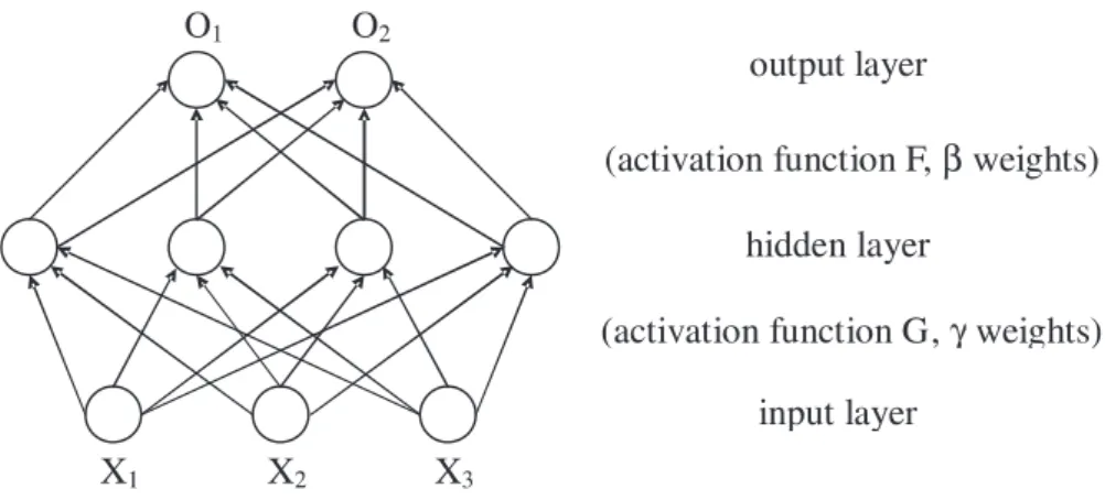
hidden units connected to all input and output units; the strengths of such connections are labeled by (unknown) parameters known as the network connection weights. In particular, γ_h = (γ_h,1, . . . , γ_h,m) denotes the vector of the connection weights between theh-th hidden unit and all m input units, andβ_j = (β_j,1, . . . , β_j,q) denotes the vector of the connection weights between the j-th output unit and allq hidden units. An ANN in which the sample information (signals) are passed forward from the input layer to the output layer without feedback is known as a feedforward neural network. Figure 1 illustrates the architecture of a 3-layer feedforward network with 3 input units, 4 hidden units and 2 output units.

Figure 1: A feedforward network with 3 input units, 4 hidden units and 2 output units.

This multi-layered structure of a feedforward network is designed to function as a biological neural system. The input units are the neurons that receive the information (stimuli) from the outside environment and pass them to the neurons in a middle layer (i.e., hidden units). These neurons then transform the input signals to generate neural signals and forward them to the neurons in the output layer. The output neurons in turn generate signals that determine the action to be taken. Note that all information from the units in one layer are processed simultaneously, rather than sequentially, by the units in an “upper” layer.1

Formally, the input units receive the information x_t and send to all hidden units, weighted by the connection weights between the input and hidden units. This information is then transformed by theactivation function Gin each hidden unit. That is, the h-th hidden unit receives x_tγ_h and transforms it to G(x_tγ_h). The information generated by all hidden units is further passed to the output units, again weighted by the connection weights, and transformed by the activation function F in each output unit. Hence, the

j-th output unit receivesq_h=1β_j,hG(x_tγ_h) and transforms it into the network output:

o_t,j =F q h=1 β_j,hG(x_tγ_h) , j = 1, . . . , n. (1)

The outputO_j is used to describe or predict the behavior of thej-th target Y_j.

In practice, it is typical to include a constant term, also known as the biasterm, in

1_{This concept, also known as parallel processing or massive parallelism, differs from the traditional}

each activation function in (1). That is, o_t,j =F β_j,0+ q h=1 β_j,hG(γ_h,0+x_tγ_h) , j= 1, . . . , n, (2)

where γ_h,0 is the bias term in the h-th hidden unit and β_j,0 is the bias term in the

j-th output unit. A constant term in each activation function adds flexibility to hidden-unit and output-hidden-unit responses (activations), in a way similar to the constant term in (non)linear regression models. Note that when there is no transformation in the output units, F is an identity function (i.e., F(a) =a) so that

o_t,j =β_j,0+

q

h=1

β_j,hG(γ_h,0+x_tγ_h), j= 1, . . . , n, (3) It is also straightforward to construct networks with two or more hidden layers. For simplicity, we will focus on the 3-layer networks with only one hidden layer.

While parametric econometric models are typically formulated using a given function of the inputx_t, the network (2) is a class of flexible nonlinear functions of x_t. The exact form of a network model depends on the activation functions (F andG) and the number of hidden units (q). In particular, the network function in (3) is an affine transformation of Gand hence may be interpreted as an expansion with the “basis” functionG.

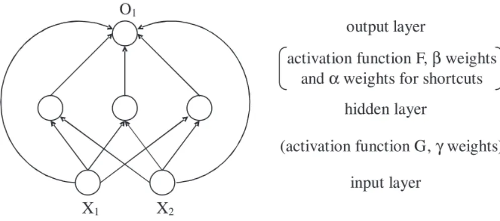
The networks (2) and (3) can be further extended. For example, one may construct a network in which the input units are connected not only to the hidden units but also directly to the output units. This leads to networks with shortcut connections. Corresponding to (2), the outputs of a feedforward network with shortcuts are

o_t,j =F β_j,0+x_tα_j + q h=1 β_j,hG(γ_h,0+x_tγ_h) , j = 1, . . . , n,

where α_j is the vector of connection weights between the output and input units. and corresponding to (3), the outputs are

o_t,j =β_j,0+x_tα_j+

q

h=1

β_j,hG(γ_h,0+x_tγ_h), j= 1, . . . , n.

Figure 2 illustrates the architecture of a feedforward network with 2 input units, 3 hidden units, 1 output unit and shortcut connections. Thus, parametric econometric models may be interpreted as feedforward networks with shortcut connections but no hidden-layer connections. The linear combination of hidden-unit activations,q_h=1β_j,hG(γ_h,0+x_tγ_h), in effect characterizes the nonlinearity not captured by the linear function of x_t.

Figure 2: A feedforward neural network with shortcuts.

2.2 Recurrent Neural Networks

From the preceding section we can see that there is no “memory” device in feedforward networks that can store the signals generated earlier. Hence, feedforward networks treat all sample information as “new;” the signals in the past do not help to identify data features, even when sample information exhibits temporal dependence. As such, a feed-forward network must be expanded to a large extent so as to represent complex dynamic patterns. This causes practical difficulty because a large network may not be easily implemented. To utilize the information from the past, it is natural to include lagged target informationy_t−k,k= 1, . . . , s, as input variables, similar to linear AR and ARX models in econometric studies. Yet, such networks do not have any built-in structure that can “memorize” previous neural responses (transformed sample information). The so-calledrecurrent neural networksovercome this difficulty by allowing internal feedbacks and hence are especially appropriate for dynamic problems.

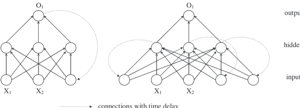
Jordan (1986) first introduced a recurrent network with feedbacks from output units. That is, the output units are connected to input units but with time delay, so that the network outputs at timet−1 are also the input information at time t. Specifically, the outputs of a Jordan network are

o_t,j =F β_j,0+ q h=1 β_j,hG(γ_h,0+x_tγ_h+o_t−1δ_h) , j= 1, . . . , n. (4)

where δ_h is the vector of the connection weights between the h-th hidden unit and the input units that receive lagged outputso_t−1 = (o_t−1,1, . . . , o_t−1,n). The network (4) can be further extended to allow for more lagged outputso_t−2,o_t−3, . . . .

Figure 3: Recurrent neural networks: Jordan (left) and Elman (right).

Similarly, Elman (1990) considered a recurrent network in which the hidden units are connected to input units with time delay. The outputs of an Elman network are:

o_t,j =F β_j,0+ q h=1 β_j,ha_t,h , j= 1, . . . , n, a_t,h =G(γ_h,0+x_tγ_h+a_t−1δ_h), h= 1, . . . , q, (5)

where a_t−1 = (a_t−1,1, . . . , a_t−1,q) is the vector of lagged hidden-unit activations, and

δ_h here is the vector of the connection weights between the h-th hidden unit and the input units that receive lagged hidden-unit activations a_t−1. The network (5) can also be extended to allow for more lagged hidden-unit activations a_t−2,a_t−3, . . . . Figure 3 illustrates the architectures of a Jordan network and an Elman network.

From (4) and (5) we can see that, by recursive substitution, the outputs of these recur-rent networks can be expressed in terms of currecur-rent and all past inputs. Such expressions are analogous to the distributed lag model or the AR representation of an ARMA model (when the inputs are lagged targets). Thus, recurrent networks incorporate the informa-tion in the past input variables without including all of them in the model. By contrast, a feedforward network requires a large number of inputs to carry such information. Note that the Jordan network and the Elman network summarize past input information in dif-ferent ways and hence have their own merits. When the previous “location” of a network is crucial in determining the next move, as in the design of a robot, a Jordan network seems more appropriate. When the past internal neural responses are more important, as in language learning problems, an Elman network may be preferred.

2.3 Choices of Activation Function

As far as model specifications are concerned, the building blocks of an ANN model are the activation functions F and G. Different choices of the activation functions result in different network models. We now introduce some activation functions commonly employed in empirical studies.

Recall that the hidden units play the role of neurons in a biological system. Thus, the activation function in each hidden unit determines whether a neuron should be turned on or off. Such an on/off response can be easily represented using an indicator (threshold) function, also known as aheaviside function in the ANN literature, i.e.,

G(γ_h,0+x_tγ_h) =

1, ifγ_h,0+x_tγ_h ≥c,

0, ifγ_h,0+x_tγ_h < c,

where c is a pre-determined threshold value. That is, depending on the strength of connection weights and input signals, the activation function G will determine whether a particular neuron is on (G(γ_h,0+x_tγ_h) = 1) or off (G(γ_h,0+x_tγ_h) = 0).

In a complex neural system, neurons need not have only an on/off response but may be in an intermediate position. This amounts to allowing the activation function to assume any value between zero and one. In the ANN literature, it is common to choose a

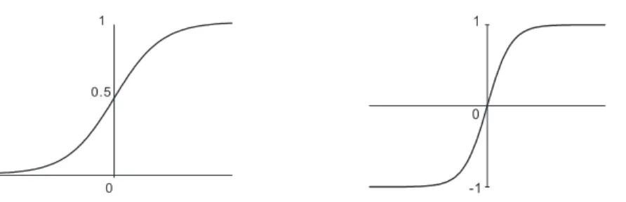
sigmoid(S-shaped) andsquashing (bounded) function. In particular, if the input signals are “squashed” between zero and one, the activation function is understood as a smooth counterpart of the indicator function. A leading example is the logistic function:

G(γ_h,0+x_tγ_h) = 1

1 + exp−[γ_h,0+x_tγ_h].

which approaches one (zero) when its argument goes to infinity (negative infinity). Hence, the logistic activation function generates a partially on/off signal based on the received input signals.

Alternatively, the hyperbolic tangent (tanh) function, which is also a sigmoid and squashing function, can serve as an activation function:

G(γ_h,0+x_tγ_h) =exp

γ_h,0+x_tγ_h−exp−[γ_h,0+x_tγ_h] expγ_h,0+x_tγ_h+ exp−[γ_h,0+x_tγ_h].

Compared to the logistic function, this function may assume negative values and is bounded between −1 and 1. It approaches 1 (−1) when its argument goes to infin-ity (minus infininfin-ity). This function is more flexible because the negative values, in effect,

Figure 4: Activation functions: logistic (left) and tanh (right).

represent “suppressing” signals from the hidden unit. See Figure 4 for an illustration of the logistic and tanh functions. Note that for the logistic functionG, a re-scaled function

Gsuch thatG(a) = 2G(a)−1 also generates values between−1 and 1 and may be used in place of the tanh function.2

The aforementioned activation functions are chosen for convenience because they are differentiable everywhere and their derivatives are easy to compute. In particular, when

Gis the logistic function, dG(a)

da =G(a)[1−G(a)];

when Gis the tanh function, dG(a) da = 2 exp(a) + exp(−a) ₂ = sech2(a).

These properties facilitate parameter estimation, as will be seen in Section 4.1. Nev-ertheless, these functions are not necessary for building proper ANNs. For example, smooth cumulative distribution functions, which are sigmoidal and squashing, are also legitimate candidates for activation function. In Section 3, it is shown that, as far as network approximation property is concerned, the activation function in hidden units does not even have to be sigmoidal, yet boundedness is usually required. Thus, sine and cosine functions can also serve as an activation function.

As for the activation function F in the output units, it is common to set it as the identity function so that the outputs of (3) enjoy the freedom of assuming any real value. This choice suffices for the network approximation property discussed in Section 3.

2_{A choice of the activation function in classification problems is the so-calledradial basis function. We}

do not discuss this choice because its argument is not an affine transformation of inputs and hence does not fit in our framework here. Moreover, the networks with this activation function provide onlylocal

When the target is a binary variable taking the values zero and one, as in a classification problem, F may be chosen as the logistic function so that the outputs of (2) must fall between zero and one, analogous to a logit model in econometrics.

3

ANN as an Universal Approximator

What makes ANN a useful econometric tool is itsuniversal approximationproperty which basically means that a multi-layered ANN with a large number of hidden units can well approximate a large class of functions. This approximation property is analogous to that of nonparametric approximators, such as polynomials and Fourier series, yet it is not shared by parametric econometric models.

To present the approximation property, we consider the network function element by element. Let f_G,q:Rm×Θ_m,q →Rdenote the network function withq hidden units, the output activation functionF being the identity function, and the hidden-unit activation functionG, i.e., f_G,q(x;θ) =β₀+ q h=1 β_hG(γ_h,0+xγ_h),

as in (3), where Θ_m,q is the parameter space whose dimension depends onm andq, and

θ ∈Θ_m,q (note that the subscripts m and q forθ are suppressed). Given the activation functionG, the collection of allf_G,q functions with differentq is:

F_G= ∞ q=1 f_G,q:f_G,q(x;θ) =β₀+ q h=1 β_hG(γ_h,0+xγ_h) ;

when the union is taken up to a finite numberN, the resulting collection is denoted as

FN

G. Intuitively, FG is capable of functional approximation because fG,q can be viewed

as an expansion with the “basis” function G and hence is similar to a nonparametric approximator.

More formally, we follow Hornik (1991) and consider two measures of the closeness between functions. First define theuniform distance between functions f and g on the set K as

d_K(f, g) = sup

x∈K |f(x)−g(x)|.

Let K denote a compact subset in Rm and C(K) denote the space of all continuous functions on K. Then,when the activation function G is continuous, bounded and non-constant, the collection F_Gis dense in C(K) for allK inRm in terms ofd_K (Theorem 2

of Hornik, 1991).3 That is, for any functionginC(K) and any ε >0, there is a network function f_G,q in F_G such that d_K(f_G,q−g) < ε. As F_GN is not dense in C(K) for any finite number N, this result shows that any continuous function can be approximated arbitrarily well on compacta by a 3-layered feedforward network f_G,q, provided that q, the number of hidden units, is sufficiently large.

Taking xas random variables, defined in the probability space with the probability measure IP, we consider the L_r-norm off(x)−g(x):

f −g_r =

Rm|f(x)−g(x)|

r_{d IP(x)}1/r_,

1 ≤ r < ∞. For r = 2 (r = 1), this is the well known measure of mean squared error (mean absolute error). Then,when the activation functionGis bounded and nonconstant, the collection F_G is dense in the L_r space (Theorem 1 of Hornik, 1991). That is, any functiong(with finiteL_r-norm) can also be well approximated by a 3-layered feedforward networkf_G,q in terms of L_r-norm whenq is sufficiently large.

It should be emphasized that the universal approximation property of a feedforward network hinges on the 3-layered architecture and the number of hidden units, but not on the activation functionper se. As stated above, the activation function in the hidden unit can be a general bounded function and does not have to be sigmoidal. Hornik (1993) provides results that permit even more general activation functions. Moreover, a feedfor-ward network with only one hidden layer suffices for such approximation property. More hidden layers may be helpful in certain applications but are not necessary for functional approximation.

Barron (1993) further derived the rate of approximation in terms of mean squared errorf−g2₂. It was shown that 3-layered feedforward networksf_G,q withGa sigmoidal function can achieve the approximation rate of order O(1/q), for which the number of parameters grows linearly with q (with the order O(mq)). This is in sharp contrast with other expansions, such as polynomial (with p the degree of the polynomial) and spline (with p the number of knots per coordinate), which yield suitable approximation when the number of parameters grows exponentially (with the order O(pm)). Thus, it is practically difficult for such expansions to approximate well when the dimension of the input space, m, is large.

3_{Hornik (1991) considered the network without the bias term in the output unit, i.e.,β}

0= 0. Yet as long as Gis not a constant function, all the results in Hornik (1991) carry over; see Stinchcombe and White (1998) for details.

4

Implementation of ANNs

In practice, when the activation functions in an ANN are chosen, it remains to estimate its connection weights (unknown parameters) and to determine a proper number of hidden units. Given that the connection weights of an ANN model are unknown, this network must be properly “trained” so as to “learn” the unknown weights. This is why parameter estimation is referred to as networklearningand the sample used for parameter estimation is referred to a training sample in the ANN literature. As the number of hidden units

q determines network complexity, finding a suitable q is known as network complexity regularization.

4.1 Model Estimation

The network parameters can be estimated by either on-line oroff-linemethods. An on-line learning algorithm is just a recursive estimation method which updates parameter estimates when new sample information becomes available. By contrast, off-line learning methods are based on fixed training samples; standard econometric estimation methods are typically off-line.

To ease the discussion of model estimation, we focus on the simple case that there is only one target variable y and the network function f_G,q. Generalization to the case with multiple target variables and vector-valued network functions is straightforward. Once the activation function G is chosen and the number of hidden units is given, f_G,q

is a nonlinear parametric model for the targety; the network with multiple outputs is a system of nonlinear models. Taking mean squared error as the criterion, the parameter vector of interest θ∗ thus minimizes

IE[y−f_G,q(x;θ)]2. (6)

It is well known that

IEy−f_G,q(x;θ)2 = IEy−E(y|x)2+ IEIE(y|x)−f_G,q(x;θ)2.

As IE(y|x) is the bestL₂predictor ofy,θ∗must also minimize the mean squared approxi-mation error: IEIE(y|x)−f_G,q(x;θ)2. This shows that, among all 3-layered feedforward networks with the activation functionGandq hidden units,f_G,q(x;θ∗) provides the best approximation to the conditional mean function.

Given a training sample of T observations, an estimator of θ∗ can be obtained by minimizing the sample counterpart of (6):

1 T T t=1 [y_t−f_G,q(x_t;θ)]2,

which is just the objective function of the nonlinear least squares (NLS) method. The NLS method is an off-line estimation method because the size of the training sample is fixed. Under very general conditions on the data and nonlinear function, it is well known that the NLS estimator is strongly consistent forθ∗ and asymptotically normally distributed; see, e.g., Gallant and White (1988).

In many ANN applications (e.g., signal processing and language learning), the train-ing sample is not fixed but constantly expands with new data. In such cases, off-line estimation may not be feasible, but on-line estimation methods, which update the pa-rameter estimates based solely on the newly available data, are computationally more tractable. Moreover, on-line estimation methods can be interpreted as “adaptive learn-ing” by biological neural systems. It should be emphasized that when there is only a given sample, as in most empirical studies in economics, recursive estimation is not to be preferred because it is, in general, statistically less efficient than the NLS method in finite samples.

Note that the parameter of interest θ∗ is the zero of the first order condition of (6): IE∇f_G,q(x;θ)y−f_G,q(x;θ)=0,

where∇f_G,q(x;θ) is the (column) gradient vector off_G,q with respect toθ. To estimate

θ∗, a recursive algorithm proposed by Rumelhart, Hinton, and Williams (1986) is ˆ

θ_t+1 = ˆθ_t+η_t∇f_G,q(x_t; ˆθ_t)y_t−f_G,q(x_t; ˆθ_t), (7) where η_t > 0 is a parameter that re-scales the adjustment term in the square bracket. It can be seen from (7) that the adjustment term is determined by the gradient descent direction and the error between the target and network output: y_t−f_G,q(x_t; ˆθ_t), and it requires only the information at time t, i.e.,y_t,x_t, and the estimate ˆθ_t.4

The algorithm (7) is known as theerror back-propagation(or simply back-propagation) algorithm in the ANN literature, because the error signal [y_t−f_G,q(x_t; ˆθ_t)] is propagated

4_{The algorithm (7) is analogous to the numerical steepest-descent algorithm. However, (7) utilizes}

only the information at time t, whereas numerical optimization algorithms are computed using all the information in a given sample and hence are off-line methods.

back through the network to determine the change of each weight. The underlying idea of this algorithm can be traced back to the classical stochastic approximationmethod in-troduced in Robins and Monro (1951). White (1989) established consistency and asymp-totic normality of ˆθ_t in (7). Note that the parameter η_t in the algorithm is known as a learning rate. For consistency of ˆθ_t, it is required that η_t satisfies ∞_t=1η_t = ∞ and

_∞

t=1η2t < ∞, e.g., ηt = 1/t. The former condition ensures that the updating process

may last indefinitely, whereas the latter implies η_t → 0 so that the adjustment in the parameter estimates can be made arbitrarily small.5

Instead of the gradient descent direction, it is natural to construct a recursive algo-rithm with a Newton search direction. Kuan and White (1994) proposed the following algorithm: H_t+1=H_t+η_t∇f_G,q(x_t; ˆθ_t)∇f_G,q(x_t; ˆθ_t)−H_t, ˆ θ_t+1= ˆθ_t+η_tH−_t+11 ∇f_G,q(x_t; ˆθ_t)y_t−f_G,q(x_t; ˆθ_t), (8)

where H_t+1 characterizes a Newton direction and is recursively updated via the first equation. Kuan and White (1994) showed that ˆθ_t in (8) is √t-consistent, statistically more efficient than ˆθ_t in (7), and asymptotically equivalent to the NLS estimator. The algorithm (8) may be implemented in different ways; for example, there is an algorithm that is algebraically equivalent to (8) but does not involve matrix inversion. See Kuan and White (1994) for more discussions on the implementation of the Newton algorithms. On the other hand, estimating recurrent networks is more cumbersome. From (4) and (5) we can see that recurrent network functions depend onθ directly and also indirectly through the presence of internal feedbacks (i.e., lagged output and lagged hidden-unit activations). The indirect dependence on parameters must be taken into account in calculating the derivatives with respect to θ. Thus, NLS optimization algorithms that require analytic derivatives are difficult to implement. Kuan, Hornik, and White (1994) proposed the dynamic back-propagationalgorithm for recurrent networks, which is anal-ogous to (7) but involves more updating equations. Kuan (1995) further proposed a Newton algorithm for recurrent networks, analogous to (8), and showed that it is √t -consistent and statistically more efficient than the dynamic back-propagation algorithm.

5_{In many applications of ANN, the learning rate is often set to a constantηo; the resulting estimate ˆθt}

loses consistency in this case. Kuan and Hornik (1991) established a convergence result based on small-ηo asymptotics.

We omit the details of these algorithms; see Kuan and Liu (1995) for an application of these estimation methods for both feedforward and recurrent networks.

Note that the NLS method and recursive algorithms all require computing the deriva-tives of the network function. Thus, a smooth and differentiable activation function, as the examples given in Section 2.3, are quite convenient for network parameter estimation. Finally, given that ANN models are highly nonlinear, it is likely that there exist multiple optima in the objective function. There is, however, no guarantee that the NLS method and the recursive estimation methods discussed above will deliver the global optimum. This is a serious problem because the dimension of the parameter space is typically large. Unfortunately, a convenient and effective method for finding the global optimum in ANN estimation is not yet available.

4.2 Model Complexity Regularization

Section 3 shows that a network modelf_G,q can approximate unknown function when the number of hidden units, q, is sufficiently large. When there is a fixed training sample, a complex network with a very large q may over fit the data. Thus, there is a trade-off between approximation capability and over-fitting in implementing ANN models.

An easy approach to regularizing the network complexity is to apply a model selec-tion criteria,6 such as Schwarz (Bayesian) information criterion (BIC), to the network models with various q. As is well known, BIC consists of two terms: one is based on model fitness, and the other penalizes model complexity. Hence, it is suitable for regu-larizing network complexity; see also Barron (1991). A different criterion introduced in Rissanen (1986, 1987) ispredictive stochastic complexity (PSC) which is just an average of squared prediction errors:

PSC = 1 T−k T t=k+1 y_t−f_G,q(x_t,θˆ_t)2,

where ˆθ_t is the predicted parameter estimate based on the sample information up to time t−1, and k is the total number of parameters in the network. Given the number of inputs, the network with the smallest BIC or PSC gives the desired number of hidden

6_{Alternatively, one may consider testing whether some hidden units may be dropped from the model.}

This amounts to testing, say, βh = 0 for some h. Unfortunately, the parameters in that hidden-unit activation function (γh,0 and γ_h) are not identified under this null hypothesis. It is well known that, when there are unidentified nuisance parameters, standard econometric tests are not applicable.

unitsq∗. Rissanen showed that both BIC and PSC can be interpreted as the criteria for “minimum description length,” in the sense that they determine the shortest code length (asymptotically) that is needed to encode a sequence of numbers. In other words, these criteria lead to the least complex model that still captures the key information in data. Swanson and White (1997) showed that a network selected by BIC need not perform well in out-of-sample forecasting, however.

Clearly, PSC requires estimating the parameters at each t. It would be computa-tionally demanding if the NLS method is to be used, even for a moderate sample. For simplicity, Kuan and Liu (1995) suggested a two-step procedure for implementing ANN models. In the first step, one estimates the network models and computes the resulting PSCs using the recursive Newton algorithm, which is asymptotically equivalent to the NLS method. When a suitable network structure is determined, the Newton parame-ter estimates can be used as initial values for NLS estimation in the second step. This approach thus maintains a balance between computational cost and estimator efficiency.

5

Concluding Remarks

In this entry, we introduce ANN model specifications, their approximation properties, and the methods for model implementation from an econometric perspective. It should be emphasized that ANN is neither a magical econometric tool nor a “black box” that can solve any difficult problems in econometrics. As discussed above, a major advantage of ANN is its universal approximation property, a property shared by other nonparametric approximators. Yet compared with parametric econometric models, a simple ANN need not perform better, and a more complex ANN (with a large number of hidden units) is more difficult to implement properly and can not be applied when there is only a small data set. Therefore, empirical applications of ANN models must be exercised with care.

References

Barron, A. R. (1991). Complexity regularization with application to artificial neural networks, inNonparametric Functional Estimation and Related Topics, G. Roussas (ed.), pp. 561–576, Dordrecht, the Netherlads: Kluwer Academic Publishers. Barron, A. R. (1993). Universal approximation bounds for superpositions of a sigmoidal

function,IEEE Transactions on Information Theory, IT-39, 930–945.

Cybenko, G. (1989). Approximation by superpositions of a sigmoid function, Mathemat-ics of Control, Signals, and Systems,2, 303–314.

Elman, J. L. (1990). Finding structure in time,Cognitive Science,14, 179-211.

Funahashi, K. (1989). On the approximate realization of continuous mappings by neural networks,Neural Networks,2, 183–192.

Gallant, A. R. and H. White (1988). A Unified Theory of Estimation and Inference for Nonlinear Dynamic Models, Oxford, UK: Basil Blackwell.

Hornik, K. (1991). Approximation capabilities of multilayer feedforward nets, Neural Networks,4, 231–242.

Hornik, K. (1993). Some new results on neural network approximation,Neural Networks,

6, 1069–1072.

Hornik, K., M. Stinchcombe, and H. White (1989). Multi-layer feedforward networks are universal approximators,Neural Networks,2, 359–366.

Hornik, K., M. Stinchcombe, and H. White (1990). Universal approximation of an un-known mapping and its derivatives using multilayer feedforward networks,Neural Networks,3, 551–560.

Jordan, M. I. (1986). Serial order: A parallel distributed processing approach, Institute for Cognitive Science Report 8604, UC San Diego.

Kuan, C.-M. (1995) “A recurrent Newton algorithm and its convergence properties”,

IEEE Transactions on Neural Networks,6, 779–783.

Kuan, C.-M. and K. Hornik (1991). Convergence of learning algorithms with constant learning rates,IEEE Transactions on Neural Networks,2, 484–489.

Kuan, C,-M., K. Hornik, and H. White (1994). A convergence result for learning in recurrent neural networks, Neural Computation,6, 420–440.

Kuan, C.-M. and T. Liu (1995). Forecasting exchange rates using feedforward and re-current neural networks,Journal of Applied Econometrics,10, 347–364.

Kuan, C.-M. and H. White (1994). Artificial neural networks: An econometric perspec-tive (with discussions),Econometric Reviews, 13, 1–91 and 139–143.

McClelland, J. L., D. E. Rumelhart, and the PDP Research Group (1986). Parallel Distributed Processing: Explorations in the Microstructure of Cognition, Vol. 2, Cambridge, MA: MIT Press.

McCulloch, W. S. and W. Pitts (1943). A logical calculus of the ideas immanent in nervous activity. Bulletin of Mathematical Biophysics,5, 115–133.

Rissanen, J. (1986). Stochastic complexity and modeling,Annals of Statistics,14, 1080– 1100.

Rissanen, J. (1987). Stochastic complexity (with discussions), Journal of the Royal Sta-tistical Society,B,49, 223–239 and 252–265.

Robbins, H. and S. Monro (1951). A stochastic approximation method,Annals of Math-ematical Statistics,22, 400–407.

Rosenblatt, F. (1958). The perception: A probabilistic model for information storage and organization in the brain,Psychological Reviews,62, 386–408.

Rumelhart, D. E., G. E. Hinton, and R. J. Williams (1986). Learning internal represen-tation by error propagation, inParallel Distributed Processing: Explorations in the Microstructure of Cognition, Vol. 1, pp. 318–362, Cambridge, MA: MIT Press.

Rumelhart, D. E., J. L. McClelland, and the PDP Research Group (1986). Parallel Distributed Processing: Explorations in the Microstructure of Cognition, Vol. 1, Cambridge, MA: MIT Press.

Stinchcombe, M. B. and H. White (1998). Consistent specification testing with nuisance parameters present only under the alternative,Econometric Theory,14, 295–325. Swanson, N. R. and H. White (1997). A model selection approach to real-time

macroe-conomic forecasting using linear models and artificial neural networks, Review of Economics and Statistics,79, 540–550.

White, H. (1988). Economic prediction using neural networks: The case of IBM stock prices. Proceedings of the Second Annual IEEE Conference on Neural Networks, pp. II:451–458. New York: IEEE Press.

White, H. (1989). Some asymptotic results for learning in single hidden layer feedforward network models,Journal of the American Statistical Association, 84, 1003–1013.

Number Author(s) Title Date 06-A010 Chung-Ming Kuan Artifcial Neural Networks 09/06 06-A009 Wei-Ming Lee Testing Over-Identifying Restrictions without Consistent 09/06 Chung-Ming Kuan Estimation of the Asymptotic Covariance Matrix

06-A008 Chung-Ming Kuan. Improved HAC Covariance Matrix Estimation 09/06

06-A007 Yu-Chin Hsu Change-Point Estimation of Nonstationary I(d) Processes 09/06 Chung-Ming Kuan

06-A006 Yuko Kinishita On the Role of Absorptive Capacity: FDI Matters to Growth 08/06

Chia-Hui Lu

06-A005 Kamhon Kan Residential Mobility and Social Capital 07/06 06-A004 Kamhon Kan Cigarette Smoking and Self –Control 07/06 06-A003 林忠正 懲罰怠惰、流失人才 06/06 06-A002 Shin-Kun Peng Spatial Competition in Variety and Number of Stores 02/06 Takatoshi Tabuchi

06-A001 Mamoru Kaneko Inductive Game Theory: A Basic Scenario 01/06 J. Jude Kline

05-A011 Amy R. Hwang An Ecological-Economic Integrated General Equilibrium Model 12/05 05-A010 Juin-jen Chang A “Managerial” Trade Union and Economic Growth 12/05 Ming-fu Shaw

Ching-chong Lai

05-A009 Lin-Ti Tan Spatial Economic Theory of Pollution Control under Stochastic 10/05 Emissions

05-A008 Kamhon KAN Entrepreneurship and Risk Aversion 10/05 Wei-Der TSAI

05-A007 江豐富 台灣縣市失業率的長期追蹤研究—1987- 2001 08/05 05-A006 Shin-Kun Peng, Economic Integration and Agglomeration in a Middle 06/05 Jacques-Francois Thisse Product Economy

Ping Wang

05-A005 譚令蒂 論藥價差 05/05 洪乙禎

謝啟瑞

05-A004 Lin-Ti Tan Spatial Monopoly Pricing in a Stochastic Environment 05/05 Yan-Shu Lin

05-A003 Been-Lon Chen Congestible Public Goods and Indeterminacy in a 03/05 Shun-Fa Lee Two-sector Endogenous Growth Model*

05-A002 C. Y. Cyrus Chu The Optimal Decoupled Liabilities: A General Analysis 02/05 Hung-Ken Chien

05-A001 Cyrus C.Y. Chu Durable-Goods Monopolists, Network Effects and 02/05 Hung-Ken Chien Penetration Pricing

04-A015 Been-Lon Chen Multiple Equilibria in a Growth Model with Habit Persistence 11/04

04-A014 C. Y. Cyrus Chu A New Model for Family Resource Allocation Among 05/04 R. R. Yu Siblings: Competition, Forbearance, and Support

Ruey S. Tsay

04-A013 C. Y. Cyrus Chu Transmission of Sex Preferences Across Generations: 05/04 Ruey S. Tsay The Allocation of Educational Resources Among Siblings

Huoying Wu

04-A012 C. Y. Cyrus Chu Children as Refrigerators: When Would Backward 05/04 Altruism Appear?

04-A011 Marcus Berliant Welfare Analysis of Number and Locations of Local 05/04 Shin-Kun Peng Public Facilities

Ping Wang

04-A010 Daigee Shaw Assessing Alternative Policies for Reducing Household 03/04 Yue-Mi Tsai Waste in Taiwan

04-A009 Daigee Shaw A Probabilistic Risk Analysis for Taipei Seismic Hazards: 03/04 Chin-Hsiung Loh An Application of HAZ-Taiwan with its Pre-processor and

Chin-Hsun Yeh Post-processor Wen-Yu Jean

Yen-lien Kuo

04-A008 Yu-Lan Chien A General Model of Starting Point Bias in Double-Bounded 03/04 Cliff J. Huang Dichotomous Contingent Valuation Surveys

Daigee Shaw

04-A007 鍾經樊 財富在不同時期對台灣消費行為的影響： 02/04

詹維玲 多變量馬可夫結構轉換模型的應用 張光亮

04-A006 Chun-chieh Huang Working Hours Reduction and Endogenous Growth 02/04 Ching-Chong Lai

Juin-Jen Chang

04-A005 Juin-Jen Chang On the Public Economics of Casino Gambling 02/04 Ching-Chong Lai

Ping Wang

04-A004 Ming-Fu Shaw Interest Rate Rules, Target Policies, and Endogenous 02/04 Shu-Hua Chen Economic Growth in an Open Economy

Ching-Chong Lai Juin-Jen Chang